Sage Journals: Discover world-class research

Abstract

A major challenge of outcomes research is measuring hospital performance using readily available administrative data. When the outcome measure is mortality or morbidity, rates are adjusted to account for preexisting conditions that may confound their assessment. However, the concept of “risk-adjusted” outcomes is frequently misunderstood. In this article, we try to clarify things, and we describe Stata tools for appropriately calculating and displaying risk-standardized outcome measures. We offer practical guidance and illustrate the application of these tools to an example based on real data (30-day mortality following acute myocardial infarction in Latvia).

Keywords

st0562 risk adjustment bootstrap caterpillar plot eclplot funnel plot generalized estimating equations healthcare quality assessment hospital profiling mfpboot mfpboot bif multivariable modeling outcomes research qic riskstandardized mortality rates stability xtgee

1 Introduction

Outcomes research frequently aims to measure the performance of a physician or a hospital. This is often called provider profiling (Gatsonis 2005). The outcome rates are generally adjusted to remove the effect of age, allowing for an unbiased comparison between populations that may differ with respect to age. Countless biostatistics and epidemiology textbooks address this topic, so the direct and indirect methods to calculate age-adjusted rates are widely known.

Things get more complicated when other variables, such as clinical factors, are accounted for to derive risk-adjusted measures. Although age is generally the main source of confounding in epidemiological studies, other characteristics can significantly impact the patient’s individual risk and are outside the quality of care delivered. These additional characteristics can be retrieved from the hospital discharge records—also known as discharge abstracts or administrative claims—which are generally inexpensive and enable the analysis of large populations as well as many conditions and pathologies. This source of data is largely used in outcome studies but is nonetheless criticized because of limited accuracy of medical billing diagnosis and procedure coding. Despite this limitation, healthcare administrative databases are rich sources of information that are being leveraged for research purposes and used for policy decision making (Cadarette and Wong 2015).

In outcomes research, risk-adjustment techniques develop from logistic regression analysis. It seems trivial at first glance, but the assumption of independence does not hold when observations are clustered within second-level units (for example, hospitals), so one must take important precautions. We also think that the literature regarding risk adjustment still lacks structure, possibly because the topic is broad, disputed, and somewhat sensitive. Risk-adjusted outcomes are used to designate centers of excellence, to determine reimbursement levels in pay for performance programs, and to classify providers as outliers, so it is no surprise that their correct conceptualization and interpretation goes beyond the strict academic concern (Shahian and Normand 2008).

For whatever reason, the result is a list of definitions and abbreviations that might confuse someone first encountering this field of statistics. In this article, we try to clarify things by explaining step by step which techniques should be used to calculate and display the risk-adjusted outcome rates. We follow key methodological concepts with details of how to run risk-adjustment models in Stata using a practical example derived from real data (30-day mortality following acute myocardial infarction [AMI] in Latvia in 2016). Because this article is addressed to all health-services professionals and researchers skilled with numbers, we do not review advanced techniques, such as Bayesian hierarchical models.

2 Risk-standardized mortality rates

2.1 Logistic regression

The easiest way to obtain risk-adjusted outcome measures across providers is to build a conventional logistic regression model, where Y is a binary outcome measure expressed as 0/1 (say, death) and covariates X_i are the patient case mix (age, sex, comorbidities, etc.). We will describe methodological details on how these variables can be selected for inclusion in the model in section 3.

Regression coefficient estimates capture the effect of patient characteristics on the study outcome across all hospitals together. The predicted probability of the outcome can be derived for each patient by combining the regression coefficients estimated by the model with the patient set of covariates. In this way, each patient has both the actual outcome and the predicted probability of that outcome accounting for risk factors identified in the model. These measures are then summed over all records within each provider to derive the observed and the expected number of events. The expected number of events is the number of events that would occur if the “standard” event rates had happened, given the actual provider case mix. Standard event rates are estimated from the entire group of providers.

The adjusted outcome measure for each provider is presented as the ratio of the observed to the expected number of events. This is called the observed-to-expected ratio or, when the events are deaths, the standardized mortality ratio (SMR) (Naing 2000). The SMR compares the outcomes for the specific distribution of patients at a hospital with their expected results had they been treated by an average provider in the reference population. The SMR is favorable if less than 1 and unfavorable if greater than 1.

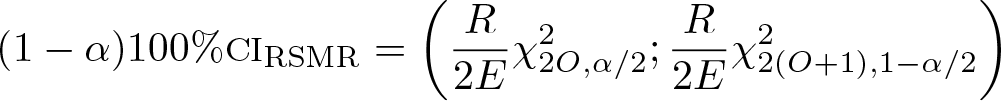
As a final step, the SMR should be multiplied by the overall outcome rate to allow for comparison of each hospital performance with the national or regional average. This measure is named either risk-standardized mortality rate (RSMR) or risk-adjusted mortality rate and is given by the following formula:

RSMR = SMR × overall mortality rate

The RSMR is favorable when it is below the overall mortality rate and unfavorable when it is above the overall mortality rate.

2.2 Confidence intervals for RSMRs

Because the RSMRs for each hospital are derived from the reference population, it is appropriate to assess whether these rates are statistically different from the overall state or region mortality rate. This is achieved by determining whether the confidence interval (CI) for a hospital-specific RSMR includes the overall rate. If no overlap exists, the hospital is most commonly classified as a statistical outlier (Shahian and Normand 2008).

The analyst will have many choices because many formulas have been proposed to build CIs. These formulas are based on the assumption that the observed deaths are Poisson variates (that is, random variables with a Poisson distribution), while the expected deaths are not variates.

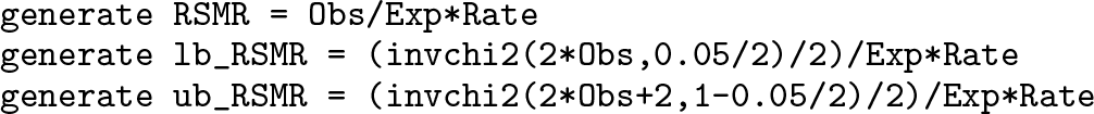
To avoid the iterative calculations needed for the exact results, we suggest constructing the CIs of RSMRs following the formula that relates the chi-squared distribution and the Poisson distribution:

(1 - α) 100 % {CI}_{RSMR} = (\frac{R}{2 E} x_{2 O, α / 2}^{2}; \frac{R}{2 E} x_{2 (O + 1), 1 - α / 2}^{2})

where O and E are, respectively, the number of observed and number of expected deaths for the provider, R is the overall mortality rate, and $χ_{_{ν, α}}^{2}$ denotes the 100αth percentile of a chi-squared distribution with ν degrees of freedom (Garwood 1936).

2.3 Generalized estimating equations

It is likely that responses of patients from within the same hospital are correlated, even after adjusting for the effects of age, sex, and other potential confounders. This positive correlation is because each hospital has a unique mixture of staff, policies, and medical culture that combine to influence patient results. Fitting conventional regression models to correlated data often leads to inefficient parameter estimates and systematically small standard errors (Houchens, Chu, and Steiner 2007). Inefficient regression estimates are more widely scattered around the true population value than they would be if the within-group correlation were incorporated in the analysis.

Generalized estimating equations (GEEs) are one of the methods that account for correlated observations. GEEs are a flexible tool that can be trivially seen as an extension of conventional regression models, such as linear, logistic, or Poisson. A working correlation matrix reflecting average dependence among correlated observations must be specified when running GEEs to improve the efficiency of the parameter estimates. In Stata, the default within-group correlation structure corresponds to the equal-correlation model, also called “exchangeable”. The equal-correlation model is appropriate for profiling studies, where no time-varying outcomes or covariates must be investigated (Ballinger 2004).

Ample literature has suggested the use of a robust estimation of standard errors (also known as sandwich or Huber–White standard errors) when conducting analyses on correlated data and especially in conjunction with GEEs (Liang and Zeger 1986). These robust estimates allow the correct specification of the mean model while relaxing the assumption of correctly specifying the form of the variance model, that is, the working correlation matrix. In other words, GEEs are generally robust to misspecification of the variance model.

A known limitation of the robust variance estimate is that it can present issues in underestimating the variance when there are not enough clusters. A rule of thumb states that with fewer than 50 clusters, there may be concern about a biased estimate, while with more than 50 clusters, the estimate is likely to be asymptotically unbiased. It is thus advisable to correct robust standard error estimates for small sample sizes by using the divisor M − P, where M is the number of hospitals and P is the number of regression parameter estimates, instead of the default M (Huang, Fiero, and Mell 2016).

2.4 GEEs versus conventional logistic regression

GEEs should be generally preferred to conventional regression models when observations are clustered within groups. However, results from GEEs and logistic regression with robust standard errors are identical if the within-group correlation is close to 0.

To test whether observations are actually correlated, one should compare a GEE model with an exchangeable working matrix and with an independent working matrix. The best model between the two has the lowest quasilikelihood under independence criterion (QIC). The QIC is an extension of the widely used Akaike information criterion for model selection in GEE analysis (Pan 2001).

2.5 Stata code

A GEE model for a binary outcome (depvar) can be fit, and individual risk factors (indepvars) can be estimated using the Stata commands displayed below. The variable varname_i uniquely identifies providers. Note that, by adding the eform option, xtgee will report odds ratios instead of regression coefficients. Before launching xtgee, the default matrix size may need to be increased (11,000 is the maximum allowed number of variables).

To compare two GEE models with different within-group correlation structures (such as exchangeable and independent), you should first download the qic package by typing ssc install qic. You can then use the qic command (Cui 2007).

The model with the lowest QIC must be preferred. If the model with an independent working matrix is the best fitting one, you can run a conventional logistic regression with clustered sandwich estimates to get the same output.

All these commands incorporate robust estimators. Of course, categorical indepvars must be preceded by i. to create dummies.

After running the best model between the two, we use predict to save in newvar the estimated individual risk for each patient using the observed values of his or her confounding variables. Note that logit postestimation asks for pr instead of rate. The expected number of events per provider can be then summarized with tabstat.

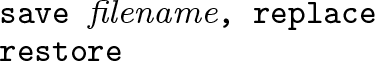
As a further step, one might want to calculate the RSMRs with 95% CIs for each hospital. To manipulate data at the hospital level, we use collapse—do not forget to launch preserve first (see [P] preserve). Let us assume that the variable containing the predicted probabilities for each patient has been named p_hat. After collapsing the total number of observed events (Obs), expected events (Exp), and patients (N) for each hospital, we generate a new variable (say, MR) containing the crude mortality rates. With the help of tabstat, we define a scalar (say, Rate) containing the overall mortality rate value that will be useful to derive the RSMRs.

Hospital-specific RSMRs (RSMR) with 95% CIs (lb_RSMR, ub_RSMR) are calculated using the following commands, which are based on the formulas described in section 2.1 and 2.2.

Before restoring the original dataset, results must be saved as a new data file. If your filename contains embedded spaces, remember to enclose it in double quotes. This data file will be used to produce plots of either crude or risk-standardized rates (see section 5).

3 Confounder selection

The choice of predictive variables in regression analysis is somewhat of an art. Ideally, specific clinical variables to be included in each outcome model should be selected from expert panels and literature reviews of existing models.

There are some predefined sets of comorbidities, such as Elixhauser’s (Quan et al. 2005), that might be adopted to risk-adjust a broad spectrum of outcomes. However, to avoid model overfitting and misclassification, only significant risk factors should be included as covariates in regression analyses, either GEE or logistic. Many automated selection methods have been proposed—we describe in detail the one suggested by Austin and Tu (2004), which has the advantage to assess the stability of estimated regression coefficients. It can be summarized in four steps:

Conditions whose prevalence is less than 1% in the population are excluded from further analyses.

Simple regression models with clustered sandwich estimators are used to analyze the crude association between each potential confounder and outcome, and variables that are significantly associated with the outcome with a significance level of P < 0.25 are selected for possible inclusion in multivariable regression.

A bootstrap backward procedure is adopted to determine which of these factors are significantly associated with the outcome in multivariable models. Using this approach, 1,000 replicated bootstrap samples are selected from the original data. In each replicated sample, age and sex are forced into the model, while a backward elimination of potential confounders is applied with a significance level of removal equal to 0.05.

Risk factors selected in at least 500 (50%) of the replicates are included as confounders in the multivariable model, from which RSMRs are then computed.

To save time, the entire procedure might be based on logistic regression models instead of GEEs. To account for potential nonlinear relationships between age and outcome, age could be either transformed or subdivided into groups of similar size. Because a bootstrap assessment is performed to determine whether a given variable truly is an independent predictor of the outcome, this procedure does not necessarily have to be regularly done unless any changes occur in coding practices or disease epidemiology.

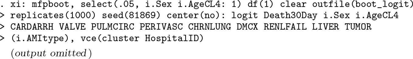
The Stata code to perform the bootstrap backward procedure is presented below. Note that the seed( # ) option should be added for reproducibility of the results. Let us say that sex and age_group are sex and age group, respectively, for each patient. The mfpboot command can be installed by typing net install mfpboot, from(http://www.homepages.ucl.ac.uk/~ucakjpr/stata) (Royston and Sauerbrei 2009).

mfpboot creates a new output file—here boot_logit.dta—with one record (the first) for the analysis of the original data and the rest for the analysis of each bootstrap sample. A summary of the resulting bootstrap inclusion fractions for each variable can be displayed by typing mfpboot_bif. Variables with a bootstrap inclusion fraction ≥ 50% will be included in the final multivariable model.

Now that the individual risk factors have been selected, GEE analysis can be run using the commands described earlier (in section 2.5). That being said, note that more advanced tools are available in the mfpboot command for stability analysis. For more details, see Royston and Sauerbrei (2009) and their other contributions to the subject.

4 Direct comparison of hospitals

Hospital-specific RSMRs are the result of an indirect form of standardization. These measures are obtained by comparing the observed mortality rates of the patients with their expected rates. The estimated rate is the “counterfactual” (Holland 1986; Rubin 2005), an ideal result obtained under a different set of hypothetical circumstances, which is the primary motivator for risk-adjustment model development (Shahian and Normand 2008).

Almost all profiling studies and public reports use indirect standardization. As anticipated, because RSMRs are derived from the overall reference population, it is most appropriate to compare the RSMRs of each individual hospital with the overall mortality rate.

Furthermore, some seek to perform a side-by-side comparison of healthcare providers. Many statisticians have developed balancing methods, such as propensity scores (Rosenbaum and Rubin 1984; D’Agostino 2007; Rubin 2007), to improve case mix balance between institutions and to justify such comparisons. Some Italian authors (Arcà et al. 2006) have recommended including provider dummies in the regression model to allow a direct form of standardization and pairwise comparisons. Currently, the Programma Nazionale Esiti uses this approach to measure hospital performance in Italy. However, RSMRs should never be used to compare one provider with another unless study design or post hoc adjustments have been shown to be successful in balancing risk factor distribution (Shahian and Normand 2008).

5 Graphical representations of RSMRs

Outcome rates can be displayed in many ways. Bar graphs, in which bar height corresponds to the provider rate, are much appreciated by healthcare consumers, interested stakeholders, and the media. However, because these plots do not operate any distinction between small and large providers, it is impossible to ascertain whether large deviations from the state average are systematic or due to chance.

A common practice of agencies for healthcare quality is to exclude small hospitals from public report cards. We discourage this approach because it gives an incomplete representation of a country’s provision of healthcare services. Two effective graphs that illustrate outcome measures across providers and incorporate sample-size information are the caterpillar plot (sometimes inaccurately referred to as the forest plot) and the funnel plot (Spiegelhalter 2005).

The caterpillar plot is a sort of league table in which providers are ranked according to a performance indicator and, with the aid of CIs (section 2.2), outlying providers are identified. To avoid data misinterpretation, the providers should never be labeled with their rank, and outlying rates must be strictly determined using CIs. The providers that serve few patients have wider CIs that are due to small sample sizes.

Plots of estimates and CIs can be obtained in Stata using the eclplot package (Newson 2003), downloadable from the Statistical Software Components archive.

Funnel plots are an alternative graphical aid for reporting outcome rates. Each hospital rate (y axis) is plotted relative to its denominator size (x axis). The control limits form a sort of funnel around the target outcome, which corresponds to the state or regional average. These boundaries are a measure of precision of the hospital rates and depend on denominator sizes. In most cases, 95% (≈ 2 standard deviation) and 99.8% (≈ 3 standard deviation) limits around the overall mortality rate are superimposed on the scatterplot. Hospitals lying outside the control limits can be seen as outliers.

Given r as the overall rate, n as the hospital volume, and z as the standard normal distribution quantile, control limits are plotted at

y_{α / 2} (r, n) = r \pm z_{α / 2} \sqrt{\frac{r (1 - r)}{n}}

where z_α/ ₂ is 1.96 for 95% control limits and 3.09 for 99.8% control limits. Alternative methods to compute control limits are described by Spiegelhalter (2005).

Funnel plots should be preferred to caterpillar plots because 1) the eye is instinctively drawn to important points that lie outside the funnel, 2) there is no spurious ranking of institutions, 3) there is allowance for additional variability in institutions with small volume, 4) the relationship of outcome with volume can be informally assessed, and most importantly, 5) pairwise comparisons between providers are naturally discouraged.

Funnel plots can be obtained using the funnelcompar command (Forni and Gini 2013) or by combining a scatterplot (twoway scatter) with two-way function plots (twoway function). In the next section, we see how to obtain customized caterpillar and funnel plots in Stata.

6 Example

As an example, we use real data from 20 hospitals in Latvia in 2016. The outcome of interest is the 30-day AMI mortality rate. Death within 30 days of hospital admission is Death30Days, expressed as 0/1, and the hospital identification number is HospitalID. A total of 2,916 patients met the study inclusion criteria. The overall mortality rate is 17.5%.

For each patient, we have collected this clinical information: ST elevation status (AMItype), history of AMI (AMIPREV), and 31 comorbidities based on the Elixhauser method, which has been shown to perform well in predicting in-hospital AMI mortality (Southern, Quan, and Ghali 2004). All these variables are expressed as 0/1 except AMItype, which comprises three categories (STEMI/NSTEMI/unspecified STEMI). Discharge data were retrieved from the hospital discharge records; deaths were retrieved from the Mortality Register Database.

First, clinical conditions whose prevalence is less than 1% must be identified and discarded from further analyses. With tabstat, we see that 13 comorbidities (PARA, HYPOTHY, AIDS, etc.) occur in fewer than 29 out of 2,916 patients:

The crude associations between each clinical condition and the outcome are analyzed using logit. For the sake of brevity, we report only results for two Elixhauser comorbidities with prevalence > 1%: congestive heart failure (CHF) and cardiac arrhythmias (CARDARRH). While CHF is not significantly associated with 30-day mortality (P = 0.806), CARDARRH is (P < 0.001):

Using mfpboot, we perform an automated model-selection procedure on conditions associated with the outcome in previous analyses (P < 0.25). These are cardiac arrhythmias (CARDARRH), valvular disease (VALVE), pulmonary circulation disorders (PULMCIRC), peripheral vascular disease (PERIVASC), chronic pulmonary disease (CHRNLUNG), diabetes with chronic complications (DMCX), renal failure (RENLFAIL), liver disease (LIVER), solid tumors without metastasis (TUMOR), and STEMI status (AMItype). The full command is presented below (please note that factor variables, such as AMItype, must be in parentheses):

The bootstrap inclusion fractions for each variable can be easily derived from the boot_logit.dta output file by typing mfpboot_bif:

Variables with nonmissing values in at least half of the replicates (≥ 500) are eligible for inclusion in the final model. These are CARDARRH, PULMCIRC, PERIVASC, DMCX, and AMItype. Age and sex are retained in each bootstrap replicate because they have been forced into the model.

The next step is to choose the best working correlation structure for the regression model. We first calculate the QIC value for the exchangeable correlation structure, and then we calculate the QIC value for the independent correlation structure. Both of the models have the covariates chosen in the previous analyses, plus age and sex. Because we have a large sample, the default matrix size must be augmented first to the maximum allowed. In this example, we use the nolog and nodisplay options to save space and suppress the display of the iteration log and regression coefficients. The output is as follows:

The exchangeable correlation structure has a QIC of 2479.168, while the independent correlation structure has a QIC of 2429.175. We conclude that conventional logistic regression is the best fitting model here:

The predicted probabilities and hospital-specific RSMRs with 95% CIs are calculated and saved in rsmr.dta by using the following command lines:

The list of hospital-specific crude rates, RSMRs, and 95% CIs can be obtained from rsmr.dta by using list. Table 1 shows the final results of our analysis.

Table 1.

Summary of volumes, crude, and risk-standardized 30-day AMI mortality rates in 20 hospitals in Latvia in 2016. The observed and expected number of deaths for each hospital are also reported.

Hospital	Patients	Observed deaths	Expected deaths	Crude rate	RSMR	RSMR Lower	95% CI Upper
1	23	6	3.3	26.1	32.2	11.8	70.0
2	38	5	6.3	13.2	13.8	4.5	32.3
3	46	14	9.5	30.4	25.8	14.1	43.3
4	234	36	35.1	15.4	18.0	12.6	24.9
5	21	3	4.1	14.3	12.7	2.6	37.2
6	102	23	20.9	22.6	19.3	12.2	28.9
7	116	28	18.0	24.1	27.3	18.1	39.4
8	35	12	6.2	34.3	33.7	17.4	58.9
9	7	4	2.1	57.1	33.2	9.0	84.9
10	26	6	4.1	23.1	25.3	9.3	55.1
11	157	22	24.8	14.0	15.5	9.7	23.5
12	52	4	8.0	7.7	8.8	2.4	22.4
13	60	14	12.2	23.3	20.1	11.0	33.8
14	709	91	124.8	12.8	12.8	10.3	15.7
15	1	0	0.3	0.0	0.0	.	200.6
16	124	31	25.3	25.0	21.4	14.6	30.4
17	849	142	152.2	16.7	16.3	13.7	19.2
18	36	17	7.9	47.2	37.8	22.0	60.5
19	182	36	30.6	19.8	20.6	14.4	28.5
20	98	16	14.4	16.3	19.5	11.1	31.6

Now we are ready to display the risk-standardized AMI mortality rates saved in rsmr.dta. The RSMR of hospital #15, with only one patient diagnosed with AMI, is removed from all graphs. The annotated Stata syntax to get a caterpillar plot on the 2016 Latvian data is shown below. Before launching eclplot, a new variable with the ranking of hospitals (Rank) must be created.

Figure 1 shows the result of these command lines. The RSMR of hospital #14 is significantly below the overall rate, while hospitals #7 and #18 have RSMR values significantly above the overall rate. There is no other statistically significant deviation from the state average.

Figure 1.

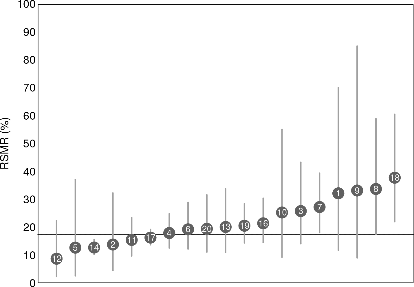
Caterpillar plot of RSMRs following AMI in 19 hospitals in Latvia in 2016. 95% CIs are plotted and compared with the overall rate of 17.5%. Hospital #15 is excluded.

Instead of using the command funnelcompar, we build a customized scatterplot with superimposed 95% and 99.8% control limits. The annotated Stata syntax for a funnel plot with the range of x axis up to 900 and the range of y axis up to 60% is shown below.

Figure 2 shows the result of these command lines. The outlying positions of hospitals #7, #14, and #18 are confirmed. In addition, hospital #8 lies just outside the upper 95% control limit. We have seen that the two plots provide similar information in terms of outlier detection, although the caterpillar plot is slightly more conservative than the funnel plot.

Figure 2.

Funnel plot of RSMRs following AMI in 19 hospitals in Latvia in 2016. The target is the overall rate of 17.5%. Hospital #15 is excluded.

7 Conclusions

In this article, we have tried to give a theoretical and methodological overview of risk adjustment and to provide some hopefully useful tips for calculating risk-standardized outcomes from regression modeling. Stata provides many powerful tools in this field of statistics, including automated model-selection techniques (mfpboot) and GEE analysis (xtgee and qic).

The RSMR of a hospital should be compared with the entire experience of a larger population of providers (that is, a country or region). Appropriate comparisons can be performed and made public with the aid of caterpillar plots, funnel plots, or both.

Supplemental Material

Supplemental Material, st0562 - Tips for calculating and displaying risk-standardized hospital outcomes in Stata

Supplemental Material, st0562 for Tips for calculating and displaying risk-standardized hospital outcomes in Stata by Jacopo Lenzi and Santa Pildava in The Stata Journal

Footnotes

8 Acknowledgments

The data presented in this article are based on work from the European Commission’s health systems performance assessment project “Developing Health System Performance Assessment for Slovenia and Latvia” (grant agreement: SRSS/S2017/019), in conjunction with the Ministry of Health of Latvia and the Management and Health Laboratory of the Sant’Anna School of Advanced Studies of Pisa, Italy.

We are grateful to Professor Sabina Nuti from the Sant’Anna School, who was appointed by the European Commission as the project leader for the Latvian health system performance assessment, and to Jana Lepiksone, head of the Research and Health Statistics Department at the Centre for Disease Prevention and Control of Latvia. We wish to thank Guido Noto, Federico Vola, and Ilaria Corazza, from the Sant’Anna School, for giving important contributions to this project. We also thank Professor Maria Pia Fantini from the University of Bologna for her inspiring lectures on outcomes research.

References

Arcà

Fusco

Barone

A. P.

Perucci

C. A.

2006. [Introduction to risk adjustment methods in comparative evaluation of outcomes]. Epidemiologia & Prevenzione 30(4–5 Suppl): 5–47.

Austin

P. C.

J. V.

2004. Bootstrap methods for developing predictive models. American Statistician 58: 131–137.

Ballinger

G. A.

2004. Using generalized estimating equations for longitudinal data analysis. Organizational Research Methods 7: 127–150.

Cadarette

S. M.

Wong

2015. An introduction to health care administrative data. Canadian Journal of Hospital Pharmacy 68: 232–237.

Cui

2007. QIC program and model selection in GEE analyses. Stata Journal 7: 209–220.

D’Agostino

R. B.

Jr.

2007. Propensity scores in cardiovascular research. Circulation 115: 2340–2343.

Forni

Gini

2013. Funnel plot for institutional comparison: The funnelcompar command. UK Stata Users Group meeting proceedings. https://www.stata.com/meeting/uk09/uk09_gini_forni.pdf.

Garwood

1936. Fiducial limits for the Poisson distribution. Biometrika 28: 437–442.

Gatsonis

C. A.

2005. Profiling providers of medical care. In Encyclopedia of Biostatistics, ed. Armitage

Colton

, 2nd ed., 4252–4254. Chichester, UK: Wiley.

10.

Holland

P. W.

1986. Statistics and causal inference. Journal of the American Statistical Association 81: 945–960.

11.

Houchens

Chu

Steiner

2007. Hierarchical modeling using HCUP data. HCUP Methods Series 2007-01, Agency for Healthcare Research and Quality. https://www.hcup-us.ahrq.gov/reports/methods/2007_01.pdf.

12.

Huang

Fiero

M. H.

Mell

M. L.

2016. Generalized estimating equations in cluster randomized trials with a small number of clusters: Review of practice and simulation study. Clinical Trials 13: 445–449.

13.

Liang

K.-Y.

Zeger

S. L.

1986. Longitudinal data analysis using generalized linear models. Biometrika 73: 13–22.

14.

Naing

N. N.

2000. Easy way to learn standardization: Direct and indirect methods. Malaysian Journal of Medical Sciences 7: 10–15.

15.

Newson

R. B.

2003. Confidence intervals and p-values for delivery to the end user. Stata Journal 3: 245–269.

16.

Pan

2001. Akaike’s information criterion in generalized estimating equations. Biometrics 57: 120–125.

17.

Quan

Sundararajan

Halfon

Fong

Burnard

Luthi

J. C.

Saunders

L. C.

Beck

C. A.

Feasby

T. E.

Ghali

W. A.

2005. Coding algorithms for defining comorbidities in ICD-9-CM and ICD-10 administrative data. Medical Care 43: 1130–1139.

18.

Rosenbaum

P. R.

Rubin

D. B.

1984. Reducing bias in observational studies using subclassification on the propensity score. Journal of the American Statistical Association 79: 516–524.

19.

Royston

Sauerbrei

2009. Bootstrap assessment of the stability of multivariable models. Stata Journal 9: 547–570.

20.

Rubin

D. B.

2005. Causal inference using potential outcomes: Design, modeling, decisions. Journal of the American Statistical Association 100: 322–331.

21.

Rubin

D. B.

. 2007. The design versus the analysis of observational studies for causal effects: Parallels with the design of randomized trials. Statistics in Medicine 26: 20–36.

22.

Shahian

D. M.

Normand

S. T.

2008. Comparison of “risk-adjusted” hospital outcomes. Circulation 117: 1955–1963.

23.

Southern

D. A.

Quan

Ghali

W. A.

2004. Comparison of the Elixhauser and Charlson/Deyo methods of comorbidity measurement in administrative data. Medical Care 42: 355–360.

24.

Spiegelhalter

D. J.

2005. Funnel plots for comparing institutional performance. Statistics in Medicine 24: 1185–1202.

Supplementary Material

Please find the following supplemental material available below.

For Open Access articles published under a Creative Commons License, all supplemental material carries the same license as the article it is associated with.

For non-Open Access articles published, all supplemental material carries a non-exclusive license, and permission requests for re-use of supplemental material or any part of supplemental material shall be sent directly to the copyright owner as specified in the copyright notice associated with the article.

0.03 MB

0.00 MB