Sage Journals: Discover world-class research

Abstract

In this article, I review recent developments of the item-count technique (also known as the unmatched-count or list-experiment technique) and introduce a new package, kict, for statistical analysis of the item-count data. This package contains four commands: kict deff performs a diagnostic test to detect the violation of an assumption underlying the item-count technique. kict ls and kict ml perform least-squares estimation and maximum likelihood estimation, respectively. Each encompasses a number of estimators, offering great flexibility for data analysis. kict pfci is a postestimation command for producing confidence intervals with better coverage based on profile likelihood. The development of the item-count technique is still ongoing. I will continue to update the kict package accordingly.

Keywords

st0559 kict kict deff kict ls kict ml kict pfci item-count technique unmatched-count technique list experiment sensitive question

1 Introduction

The item-count technique (also known as the unmatched-count or list-experiment technique) is a questioning technique for eliciting truthful responses to sensitive survey questions. The standard design for the item-count technique randomizes a survey sample into two groups. One group receives a list of items (that is, statements), while the other receives the same list plus an item that addresses a sensitive issue of interest to researchers. Instead of answering each item separately and directly, respondents report the number of items that fit certain criteria (for example, counting the items with which a respondent agrees). The item-count technique ensures the privacy and confidentiality of responses to the sensitive issue, thereby reducing respondents’ motives for deliberate misreporting. Furthermore, it still provides researchers with sufficient information for statistical inferences about the sensitive issue.

The item-count technique is becoming increasingly popular in various disciplines as a promising means of studying sensitive issues (Von Hermanni [2016]; Wolter and Laier [2014]; compare Gelman [2014]). However, data analysis for this technique is not straightforward and requires special methods that have not been built in most statistical software suites. I aim to fill this gap by introducing a new package—kict. This article proceeds as follows. In section 2, I elaborate on the item-count technique and review commonly used methods for data analysis. Many of those methods were developed for the standard item-count technique. I modify them for nonstandard item-count techniques. In section 3, I introduce the package kict. In section 4, I demonstrate its usage by replicating several studies of the item-count technique. I also highlight some practical considerations that are crucial to the applications of the item-count technique but have not received adequate attention in the literature. Finally, I conclude with remarks on the future development of the kict package.

2 The item-count technique

2.1 Basic idea

The item-count technique is essentially an encryption scheme that allows survey respondents to encode their answers to a sensitive question. Once encrypted, their answers can be deciphered only at a certain aggregate level for analysis (for example, the mean of a group of respondents’ answers). Therefore, it is safe for respondents to answer the sensitive question truthfully.¹

The 1991 National Race and Politics Survey (Sniderman, Tetlock, and Piazza 1991) is a classic example for illustrating the item-count technique. To measure the prevalence of racial prejudice among white Americans, the survey randomly divides a sample into two. Half the respondents (hereafter the “shortlist group”) are prompted with a question as follows:

“Now I’m going to read you [several] things that sometimes make people angry or upset. After I read [them] all, just tell me HOW MANY of them upset you. I don’t want to know which ones, just how many.

the federal government increasing the tax on gasoline;

professional athletes getting million-dollar-plus salaries;

large corporations polluting the environment.

How many, if any, of these things upset you?”

The other half (hereafter the “longlist group”) are prompted with the same list plus an item of interest (hereafter a “sensitive item” or “key item” as opposed to the three nonkey items above):

“a black family moving in next door.”

Racism is a sensitive issue in most modern societies. People who are upset about having new black neighbors may be reluctant to admit it publicly. Therefore, the itemcount question above asks respondents not to answer each item separately but to report the number of items that upset them, thereby allowing respondents to encrypt their answers to the sensitive item. Suppose that a respondent in the longlist group gives an answer of “two”; no one—not even the interviewer—can possibly know whether the answer counted in the key item (because it could be either two nonkey items or one nonkey item plus the key item).²

The simplest tool to decrypt the item-count data is a difference-in-means estimator. For example, if the longlist group reports that, on average, 2.20 items upset them, and the shortlist group’s average count is 2.13, then the estimated prevalence of racial prejudice is 2.20 minus 2.13—that is, 7% of white Americans would be upset about a black family moving in next door.

2.2 Methods for data analysis

Consider a simple random sample of n respondents. Let T_i be the group indicator for respondent i, where T_i = 1 if the respondent is assigned to the longlist group and T_i = 0 otherwise. Let S_i and R_i,j be respondent i’s potential answers to the key item and to the jth nonkey item, respectively (where there are J nonkey items). Take the study of racial prejudice as an example: S_i = 1 if a black family moving in next door angers respondent i and S_i = 0 otherwise. Similarly, R_i, ₂ = 1, if professional athletes getting million-dollar-plus salaries angers respondent i, and R_i, ₂ = 0 otherwise. By design, S_i and R_i,j are unobserved. The observed variable is the number of affirmative answers: Y_i = T_iS_i + R_i , where $R_{i} = \sum_{j = 1}^{J} R_{i, j} .$

Under three assumptions—treatment randomization, no design effect, and no liar— any difference between the two groups’ average counts is attributed to the key item.³ This justifies the use of the difference-in-means estimator, (1), to estimate the prevalence of the key item in the population. (Note that all estimators reviewed in this article rest on at least these three assumptions.)

E (S_{i}) = P (S_{i} = 1) = \frac{\sum_{i = 1}^{n} Y_{i} T_{i}}{\sum_{i = 1}^{n} T_{i}} - \frac{\sum_{i = 1}^{n} Y_{i} (1 - T_{i})}{\sum_{i = 1}^{n} (1 - T_{i})}

The difference-in-means estimate is identical to the slope coefficient of a simple linear regression of Y_i on T_i . Holbrook and Krosnick (2010, 53–54) generalize this connection from univariate analysis to multivariate modeling. To model S_i , they regress Y_i on T_i , a set of covariates X _i , and interaction terms between T_i and each of X _i . Equation (2) illustrates this method by a single covariate case. The coefficient of the interaction term δ_β estimates the relative prevalence of the key item among the subpopulation of X = x.

Y_{i} = γ_{α} + γ_{β} X_{i} + T_{i} (δ_{α} + δ_{β} X_{i}) + \in_{i}

NOTES:

$\begin{array}{l} γ α + γ β X i = E (Y i | X i, T i = 0) . \\ δ α + δ β X i = E (Y i | X i, T i = 1) - E (Y i | X i, T i = 0) = E (S i | X i) = P (S i = 1 | X i) . \end{array}$

Additional assumption: E(∊i|Xi, Ti) = 0.

Holbrook and Krosnick’s (2010) method is essentially a linear probability model and so may produce nonsensical predicted values—that is, the predicted probability of answering the key item affirmatively, $\hat{P}$ (S_i = 1|X _i = x), may be outside the interval between 0 and 1. Imai (2011, 409) overcomes this drawback using the nonlinear leastsquares regression. Equation (3), for example, is a nonlinear version of (2), in which the logistic function restricts predicted probabilities within the unit interval.

Y_{i} = J {(1 + e^{- γ_{α} - γ_{β} X_{i}})}^{- 1} + T_{i} {(1 + e^{- δ_{α} - δ_{β} X_{i}})}^{- 1} + \in_{i}

NOTES:

$\begin{array}{l} (1 + e^{- γ} α^{- γ} β^{X} i) - 1 = E (Y i | X i, T i = 0) / J \\ (1 + e^{- δ} α^{- δ} β^{X} i) - 1 = E (S i | X i) = P (S i = 1 | X i) . \end{array}$

Additional assumption: E(∊i|Xi, Ti) = 0.

Imai (2011, 409–411) also derives a maximum likelihood estimator as a more statistically efficient alternative to the nonlinear least-squares estimator. Note that S_i and R_i , though unobserved, are mutually identifiable (Glynn 2013, 163). For instance, given Y_i = 2 and T_i = 1, (S_i, R_i ) must be either (1, 1) or (0, 1), and the probabilities of these combinations are also identifiable. Therefore, Imai proposes modeling the joint probability of S_i and R_i . Because S_i is the primary focus, Imai factorizes the joint probability as P (R_i |S_i, X _i )P (S_i |X _i )—the estimates of the second term represent the association between respondents’ characteristics and their answers to the key item. Equation (4) shows the likelihood function of this estimator, where ψ _s and δ are coefficients to be estimated:

\prod_{i = 1}^{n} \sum_{s = 0}^{1} {P (R_{i} = Y_{i} - s T_{i} | S_{i} = s, X_{i} = x, ψ_{s}) P (S_{i} = s | X_{i} = x, δ) \times {(1_{Y_{i} \neq J + 1})}^{1 - s} {(1_{Y_{i} \neq 0 \cup T_{i = 1}})}^{s}}

NOTES:

1 _Condition = 1 if Condition holds; 1 _Condition = 0 otherwise.

Additional assumption: the distribution of R_i . For example, specifying a binomial distribution for R_i is equivalent to assuming (R_i,j ⊥ R_i,k |S_i, X _i) and P (R_i,j = 1|S_i, X _i) = P (R_i,k = 1|S_i, X _i), where j = k.

2.3 Nonstandard designs

The dual-list item-count technique

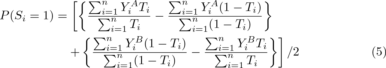
The standard item-count technique does not require the shortlist group to provide information about the key item, so the item-count estimates tend to be less precise (that is, have higher standard errors) than the estimates based on direct questioning. Droitcour et al. (1991, 189) partly overcome this limitation with a dual-list design. Consider the study of racial prejudice again. Suppose that, in addition to the original item-count question (labeled as Q^A ), we use another two nonkey items, together with the same key item, to form a second item-count question (Q^B ). As illustrated in table 1, there are still two random subgroups: group 0 answers to the short list of Q^A and then the long list of Q^B ; in contrast, group 1 answers to the long list of Q^A and then the short list of Q^B . This design prompts respondents with the key item in either Q^A or Q^B . All respondents, regardless of group, have to provide information about the key item.

Table 1.

An example of the dual-list design

Group 0 (T_i = 0)	Group 1 (T_i = 1)
Q^A I’m going to read you three things that sometimes make people angry or upset. After I read all three, just tell me how many of them upset you. I don’t want to know which ones, just how many. the federal government increasing the tax on gasoline; professional athletes getting million-dollar-plus salaries; large corporations polluting the environment. How many, if any, of these things upset you?	I’m going to read you four things that sometimes make people angry or upset. After I read all four, just tell me how many of them upset you. I don’t want to know which ones, just how many. the federal government increasing the tax on gasoline; professional athletes getting million-dollar-plus salaries; large corporations polluting the environment; a black family moving in next door. How many, if any, of these things upset you?
Q^B I’m going to read you another three things that sometimes make people angry or upset. After I read them, tell me how many of them upset you. the state government installing more speed cameras; fast food restaurant chains using horse meat in products; a black family moving in next door. How many, if any, of these things upset you?	I’m going to read you another two things that sometimes make people angry or upset. After I read them, tell me how many of them upset you. the state government installing more speed cameras; fast food restaurant chains using horse meat in products; How many, if any, of these things upset you?

For data analysis, Droitcour et al. (1991) propose applying the difference-in-means estimator to Q^A and Q^B separately to produce two estimates for the key item and then taking their arithmetic mean to obtain a more statistical efficient estimate. Formally, let Y_i ^A and Y_i ^B be respondent i’s answers to Q^A and Q^B , respectively. T_i is still the group indicator, but now T_i = 0 if respondent i is assigned to group 0 and T_i = 1 if he or she is in group 1. Equation (5) shows the difference-in-means estimator for the dual-list item-count technique.

P (S_{i} = 1) = [{\frac{\sum_{i = 1}^{n} Y_{i}^{A} T_{i}}{\sum_{i = 1}^{n} T_{i}} - \frac{\sum_{i = 1}^{n} Y_{i}^{A} (1 - T_{i})}{\sum_{i = 1}^{n} (1 - T_{i})} + \frac{\sum_{i = 1}^{n} Y_{i}^{B} (1 - T_{i})}{\sum_{i = 1}^{n} (1 - T_{i})} - \frac{\sum_{i = 1}^{n} Y_{i}^{B} T_{i}}{\sum_{i = 1}^{n} T_{i}}}] / 2

There is a lack of methods for multivariate analysis. To meet this need, I extend the methods reviewed in section 2.2 to the dual-list item-count technique (see the appendix).

The partial item-count technique

Corstange (2009) was among the first to develop a regression method for the itemcount technique. However, unlike those reviewed previously, Corstange’s (2009) method requires a nonstandard item-count design. His design (hereafter “partial item count”) requires respondents in the shortlist group to answer each nonkey item separately and directly (while those in the longlist group still answer to the question in the item-count format). Information on each nonkey item is then used to resolve the issue of model identification.

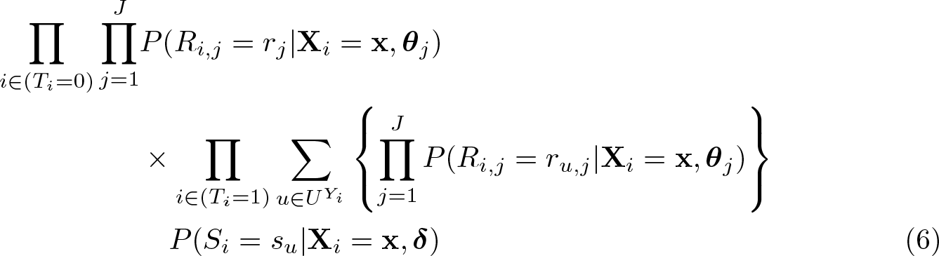
Unlike Imai’s (2011) maximum likelihood estimator that models the joint probabilities of S_i and R_i , the partial item-count technique allows Corstange (2009) to model the marginal probabilities of S_i and each R_i,j simultaneously (the primary focus is still S_i ). Corstange (2009, 51) originally devised his estimator based on an approximate likelihood function. Blair and Imai (2012, 57) improve it by deriving an exact likelihood function as shown in (6) ( θ _j and δ are coefficients to be estimated):

\prod_{i \in (T_{i} = 0)} \prod_{j = 1}^{J} P (R_{i, j} = r_{j} | X_{i} = x, θ_{j}) \times \prod_{i \in (T_{i} = 0)} \sum_{{u \in U}^{Y_{i}}} {\prod_{j = 1}^{J} P (R_{i, j} = r_{u, j} | X_{i} = x θ_{j})} P (S_{i} = s_{u} | X_{i} = x, δ)

NOTES:

U^Y ⁱ is a set of combinations of S_i and R_i,j that satisfy S_i + R_i = Y_i .

u is one of the combinations in U^Y_i .

s_u = 1 if S_i = 1 in u, and s_u = 0 otherwise.

r_u,j = 1 if R_i,j = 1 in u, and r_u,j = 0 otherwise.

Additional assumption:

S_i , R_i,j , and R_i,k (where j 6= k) are independent after controlling for X _i.

The item-sum technique

All the item-count techniques reviewed thus far require researchers to phrase the sensitive question as a dichotomous item (yes or no, agree or disagree, etc.) Trappmann et al. (2014) overcome this limitation using the item-sum technique. The item-sum technique differs from the item-count technique in two aspects: first, the key and nonkey items can be continuous variables; second, each respondent reports the sum of his or her answers to the items on the list. For example, Trappmann et al. (2014) in their study, prompted the shortlist group with two items as follows:

“Please answer each of the following questions truthfully. However, please keep the pencil and the piece of article ready. Please note the answer to each question on your piece of article. Afterward, please add the numbers from both answers together and tell me the total result. However, please do not tell me how you answered the individual questions so that I, as interviewer, do not know how you came to your result.

How many hours did you watch TV last week?

How high are your monthly costs for your apartment or your house?

Monthly costs can include rent, utilities, coop or condo fees, and mortgage.

Thank you very much. What is your result?”

The longlist group was prompted with the same questions plus a key item:

“On average, how much do you earn per month from undeclared work?”

Suppose that a respondent in the longlist group watched television 10.5 hours last week, spent €430 for his or her house per month, and made €100 from undeclared work per week; he or she is expected to give an answer of 540.5. The difference-in-means estimator (1) and the linear least-squares estimator (2) are directly applicable to the item-sum technique. For instance, if the shortlist group’s average response is 516.4, and the longlist group’s is 664.3, the estimated earnings per month from undeclared work is e147.9.

2.4 Auxiliary information

Aronow et al. (2015) consider a scenario where a survey measures a sensitive issue not only by the item-count technique but also by direct questioning. For example, besides the item-count question mentioned at the beginning of section 2.1, the 1991 National Race and Politics Survey might have also asked every respondent a direct question on the key item, such as “Does a black family moving in next door make you upset? Yes/No.” Thus, the longlist group would have answered the key item twice. With this design, Aronow et al. (2015) propose using the answers to the direct question as auxiliary information to increase the statistical efficiency of the item-count estimation.

Formally, let A_i be respondent i’s answer to the direct question, where A_i = 1 for the affirmative answer and A_i = 0 otherwise. Aronow et al. (2015) make two assumptions about this variable: 1) A_i is independent of T_i , and 2) A_i is monotonically related to S_i . As illustrated in table 2, positive monotonicity means that respondents do not answer the key item affirmatively to the item-count question while answering the direct question negatively; that is, P (S_i = 1, A_i = 0) = 0; by contrast, negative monotonicity means P (S_i = 0, A_i = 1) = 0.

Table 2.

Assumptions about the relationship between S and A

	Positive monotonicity		Negative monotonicity
	A = 0	A = 1	A = 0	A = 1
S = 0	P (S = 0, A = 0)	P (S = 0, A = 1)	P (S = 0, A = 0)	0
S = 1	0	P (S = 1, A = 1)	P (S = 1, A = 0)	P (S = 1, A = 1)

Under the negative monotonicity assumption, Aronow et al. (2015) modify the difference-in-means estimator as (7) for using A_i to aid the estimation of S_i .

P (S_{i} = 1) = (\sum_{i = 1}^{n} \frac{A_{i}}{n}) + (\sum_{i = 1}^{n} \frac{1 - A_{i}}{n}) \times {\frac{\sum_{i = 1}^{n} (1 - A_{i})}{\sum_{i = 1}^{n} T_{i} (1 - A_{i})} - \frac{\sum_{i = 1}^{n} Y_{i} (1 - T_{i}) (1 - A_{i})}{\sum_{i = 1}^{n} T_{i} T_{i} (1 - T_{i}) (1 - A_{i})}}

NOTES: Additional assumptions:

A_i is independent of T_i .

A_i is related to S_i in a negatively monotonic manner.

Equation (8) is the counterpart under the positive monotonicity assumption:

P (S_{i} = 1) = (\sum_{i = 1}^{n} \frac{A_{i}}{n}) {\frac{\sum_{i = 1}^{n} Y_{i} T_{i} A_{i}}{\sum_{i = 1}^{n} T_{i} A_{i}} - \frac{\sum_{i = 1}^{n} Y_{i} (1 - T_{i}) A_{i}}{\sum_{i = 1}^{n} (1 - T_{i}) A_{i}}}

NOTES: Additional assumptions:

A_i is independent of T_i .

A_i is related to S_i in a positively monotonic manner.

Eady (2017) uses the same type of auxiliary information to improve Imai’s (2011) maximum likelihood estimator. Like Aronow et al. (2015), Eady also assumes that A_i is monotonically related to S_i . This assumption—though simplifying estimation— severely restricts the choice of auxiliary information. Except for a direct question on the sensitive issue of interest, it is hard to see another source of auxiliary information that could possibly satisfy the monotonicity assumption. This is a major limitation of Aronow et al.’s and Eady’s methods because surveys cannot afford to adopt both a direct and an indirect approach for the same question.

Nonetheless, Tsai (2017, in part Not just unbiased but precise: How auxiliary information can improve modeling based on the item-count technique) shows that the monotonicity assumption is not essential. In fact, any individual-level information that is predictive of but extraneous to the sensitive issue of interest has the potential to improve the item-count estimation. “Extraneity” means that A_i is not a regressor for modeling S_i . (Eady also implicitly makes this assumption.) “Predictivity” requires A_i to be statistically correlated with S_i ; this assumption is weaker than monotonicity and thus places fewer restrictions on the choice of auxiliary information. (Besides, A_i still has to be independent of T_i , but this assumption is statistically testable.)

Consider the 1991 National Race and Politics Survey again. Actually, it did not include a direct question on the sensitive issue of interest, but there were other sources of auxiliary information. For example, a question in that survey asked respondents: “How do you feel about blacks buying houses in white suburbs? Strongly in favor/Somewhat in favor/Somewhat opposed/Strongly opposed.” This house-buying question and the key item of the item-count question (that is, “a black family moving in next door [makes you upset]”) are largely tautological, so it is reasonable to expect some correlation between respondents’ answers to these questions (predictivity). Also because of tautology, it is unnecessary to include that house-buying variable as a regressor to model the key item (extraneity). If the independence assumption holds too, then it is legitimate to dichotomize that variable and use it to improve the item-count estimation. (Note that the monotonicity assumption is not an essential concern.)

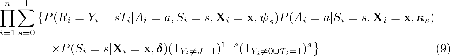
Equation (9) shows the likelihood function of Tsai’s (2017) estimator, where ψ _s , κ _s , and δ are coefficients to be estimated:

\prod_{i = 1}^{n} \sum_{s = 0}^{1} {P (R_{i} = Y_{i} - s T_{i} | A_{i} = a, S_{i} = s, X_{i} = x, ψ_{s}) P (A_{i} = a | S_{i} = s, X_{i} = x, κ_{s}) \times P (S_{i} = s | X_{i} = x, δ) {(1_{Y_{i} \neq J + 1})}^{1 - s} {(1_{Y_{i} \neq 0 \cup T_{i} = 1})}^{s}}

NOTES:

1 _Condition = 1 if Condition holds; 1 _Condition = 0 otherwise.

Additional assumptions:

A_i is independent of T_i .

A_i is predictive of S_i .

A_i is extraneous to S_i .

Distributional assumptions of R_i .

This estimator models the factorized joint probability of R_i , A_i , and S_i . As always, the coefficient δ is the primary focus; it estimates the association between respondents’ characteristics and their answers to the sensitive issue. Eady’s (2017) estimator—which rests on the assumption of either negative monotonicity, P (A_i = 1|S_i = 0, X _i, κ _s ) = 0, or positive monotonicity, P (A_i = 1|S_i = 1, X _i, κ _s ) = 1—is a special case of Tsai’s (2017) estimator.

Equation (9) is specific for the standard design of the item-count technique, but its idea applies to nonstandard designs too. In the appendix, I extend that estimator to Corstange’s (2009) partial item-count technique.

3 Commands

kict contains four commands: kict deff tests for the assumption of no design effect; kict ls performs least-squares estimation described in (1), (2), (3), (5), (7), (8), and (15); kict ml performs maximum likelihood estimation described in (4), (6), (9), (16), and (17); kict pfci estimates profile-likelihood confidence intervals (CI) for a regression coefficient yielded by kict ml. This section provides an overview of these commands.

3.1 Syntax

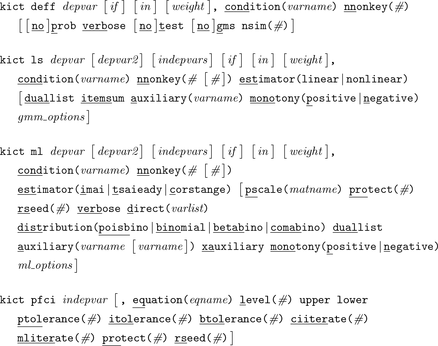
indepvar specifies an independent variable of the active kict ml model.

depvar specifies a variable that records respondents’ answers to an item-count question (Y_i ). For the dual-list design, depvar and depvar2 specify variables that record respondents’ answers to the first and second item-count questions, respectively (that is, $Y_{i}^{A}$ for Q^A and $Y_{i}^{B}$ for Q^B ). fweights, iweights, and pweights are allowed; see [U] 11.1.6 weight. Because kict is programmed using Stata’s gmm and ml, many options of these two official commands are also allowed; see [R] ml, [R] gmm, and the help files of kict in Stata.

3.2 Options for kict deff

condition( varname ) specifies a dummy variable that identifies the treatment status (T_i ). The dummy takes on the value 0, representing the shortlist group, or 1, representing the longlist group. condition() is required.

nnonkey( # ) specifies a positive integer that represents the number of nonkey items. nnonkey() is required.

[no] prob displays the estimated joint probabilities of a respondent’s answer to the key item (S_i ) and the number of nonkey items that the respondent would answer in the affirmative (R_i ). kict deff estimates the joint probabilities based on Glynn’s (2013, 166) formula.

verbose displays the computational log of the joint probabilities.

[no] test performs a test for design effects developed by Blair and Imai (2012, 64–65, 74). The null hypothesis of the test states that all the estimated joint probabilities are positive, whereas the alternative hypothesis states that any of the estimated joint probabilities are negative.

By definition, probabilities cannot be negative. If some of the estimated joint probabilities are negative, kict deff performs the test to check whether those negative estimates have arisen by chance. Rejection of the null hypothesis indicates the presence of design effects. Consequently, the estimates based on the item-count technique are questionable.

kict deff splits the estimated joint probabilities into two sets and tests them separately. The first set includes the probabilities Pr(R = 0, S = 0), Pr(R = 1, S = 0),…, Pr(R = J, S = 0), and the second set includes Pr(R = 0, S = 1), Pr(R = 1, S = 1),…, Pr(R = J, S = 1). (See also Kudo [1963].)

[[no]]gms performs the test with the method of generalized moment selection. Blair and Imai (2012, 64–65, 74) proposed using this method to improve the power of the test. The basic idea behind this method is to exclude the joint probabilities that are clearly larger than zero from the test. (See also Andrews and Soares [2010, 129, 135].)

nsim( # ) performs # Monte Carlo simulations to compute p-values when analytical solutions are not viable. The default is nsim(1000).

3.3 Options for kict ls

condition( varname ) specifies a dummy variable that identifies the treatment status. For the dual-list design, the dummy takes on the value 0 for those in the shortlist group of the first item-count question and in the longlist group of the second item-count question. However, the dummy takes on the value 1 for those in the longlist group of the first item-count question and in the shortlist group of the second item-count question (see table 1). condition() is required.

nnonkey( # [#] ) specifies a positive integer that represents the number of nonkey items. For the dual-list design, specify two positive integers that represent the numbers of the nonkey items in the first and second item-questions, respectively. (The order of the numbers matters!) nnonkey() is required.

estimator(linear| nonlinear) specifies the type of least-squares estimator to be used. linear performs the linear least-squares estimation [for example, (1) and (2)]; nonlinear performs the nonlinear least-squares estimation [for example, (3)]. estimator() is required.

duallist specifies that kict ls perform estimation for the dual-list design of the itemcount technique [for example, (5) and (15)].

itemsum specifies that kict ls perform estimation for the item-sum technique. This option pertains only to estimator(linear).

auxiliary( varname ) specifies an auxiliary variable for improving the linear leastsquares estimation for the standard item-count technique [that is, (7) and (8)]. This option pertains only to estimator(linear) and requires monotony().

monotony(positive| negative) specifies that kict ls perform estimation under a monotonicity assumption. The positive monotonicity assumes that P (A_i = 0, S_i = 1) = 0; the negative monotonicity assumes that P (A_i = 1, S_i = 0) = 0 (see table 2).

gmm_options; see help kict ls for a list of options, and see [R] gmm for option descriptions.

3.4 Options for kict ml

condition( varname ) and nnonkey( # [ # ]); see the above descriptions. condition() and nnonkey() are required.

estimator(imai| tsaieady| corstange) specifies the type of maximum likelihood estimator to be used. imai performs (4); tsaieady performs (9); corstange performs (6). estimator() is required.

pscale( matname ) specifies a row vector of positive numbers to be used as the scale parameters of Cauchy distributions. kict ml uses this vector (and fixes location parameters at zero) to construct priors and performs the quasi-Bayesian estimation. The row length of the vector must equal the number of coefficients.

Consider a vector v = [10, ., 15]. Specifying pscale(v) imposes a Cauchy(0, 10) prior on the first coefficient, a Cauchy(0, 15) prior on the third coefficient, and no prior on the second coefficient.

protect( # ) specifies that kict ml perform # optimizations with random-selected initial values and report the result with the maximum likelihood. Specifying a large number such as protect(50) provides reasonable assurance that the result found is global rather than just a local maximum.

rseed( # ) specifies the random-number seed for the option protect( # ). If the seed is not specified, the random-number generator starts in whatever state it was last in.

verbose displays iteration logs of the log likelihood when protect( # ) is specified. (Compare [no] log, which controls the iteration display for each optimization.)

ml_options; see help kict ml for a list of options, and see [R] maximize and [R] estimation options for option descriptions.

Options specific to estimator(corstange)

direct( varlist ) specifies J dummy variables; each records the shortlist group’s answers to a nonkey item. These dummies may be 0, indicating a negative outcome, or 1, indicating a positive outcome.

distribution(poisbino| binomial) specifies whether kict ml uses Corstange’s approximate likelihood function or Blair and Imai’s exact likelihood function in estimation. The default is distribution(poisbino).

The approximate likelihood function assumes that the number of affirmative answers to the key and nonkey items (S_i +R_i ) is binomially distributed (binomial), whereas the exact likelihood function uses the Poisson-binomial distribution (poisbino).

Options specific to estimator(imai)

duallist specifies that kict ml perform estimation for the dual-list design of the itemcount technique [that is, (16)].

distribution(binomial| betabino| comabino) specifies the distribution of respondents’ answers to nonkey items. The default is distribution(binomial).

Options specific to estimator(tsaieady)

auxiliary( varname varname ) specifies a dummy variable to be the auxiliary variable (A_i ). This dummy acts both as a dependent variable in the kappa0 and kappa1 equations and as a covariate in the Psi0p and Psi1p equations (or in the Thetaj equation).

If a recoded version of the dummy is also specified after the original dummy, kict ml uses the first variable as the dependent variable and uses the second one as the covariate.

xauxiliary specifies that kict ml add interaction terms between the auxiliary variable (A_i ) and every one of the covariates (X _i ) into the Psi0p and Psi1p equations (or the Thetaj equation).

monotony(positive| negative) specifies that kict ml perform estimation under one of the monotony assumptions. The positive monotonicity assumes that P (A_i = 0, S_i = 1) = 0; the negative monotonicity assumes that P (A_i = 1, S_i = 0) = 0 (see table 2).

3.5 Options for kict pfci

equation( eqname )specifies an equation name of the active kict ml model. kict pfci estimates the profile-likelihood CI for the coefficient b[ eqname : indepvar ]. The default is equation(Delta).

level( # ) sets the confidence level to be estimated. The default is level(95).

upper and lower specify kict pfci to estimate the upper and the lower limit CI, respectively. The default is estimation of both limits.

ptolerance( # ), itolerance( # ), btolerance( # ), and ciiterate( # ) specify convergence and stopping criteria.

ptolerance() specifies the difference between the targeted log likelihood and the log likelihood of the kict ml model in the current kict pfci iteration. kict pfci declares convergence if abs(ptolerance()) ≤ #. The default is ptolerance(0).

itolerance() specifies the difference in the log likelihood of the kict ml model between the previous and the current kict pfci iteration. kict pfci declares convergence if abs(itolerance()) ≤ #. The default is itolerance(0).

btolerance() specifies the difference in the coefficient b[ eqname : indepvar ] between the previous and the current kict pfci iteration. kict pfci declares convergence if abs(btolerance()) ≤ #. The default is btolerance(1e-5).

ciiterate() specifies the maximum number of kict pfci iterations.

mliterate( # ), protect( # ), and rseed( # ) change the setup that was used in estimation of the active kict ml model. Specifically, kict pfci computes CI by refitting the model in each iteration. These three options allow kict pfci to execute kictml using a different setup. See help kict ml for detailed descriptions of these options. (mliterate( # ) is the iterate( # ) in kict ml.)

4 Examples and technical details

In this section, I demonstrate the use of kict. I also provide further technical details and practical considerations about the applications of the methods reviewed previously.

4.1 The standard item-count technique

I first revisit the item-count question in the 1991 American National Race and Politics Survey. The data contain an indicator variable (group) that takes the value 0 or 1 to indicate whether a respondent is in the shortlist or longlist group. The item-count response (itemcount) takes an integer ranging from 0 to 4 because there is one key item and three nonkey items. There are also several demographic variables, including residential region (southerner versus others), age (divided by 100), gender (male or not), education level (college educated and higher versus others). After casewise deletion, 1,213 white respondents are available for analysis.⁴

Diagnostics

The validity of the item-count technique rests on at least three assumptions (footnote 3). A common practice to check the first assumption—treatment randomization—is to test for differences between the shortlist and longlist groups’ responses to important variables in the survey. No significant difference between groups indicates an effective randomization of treatment.

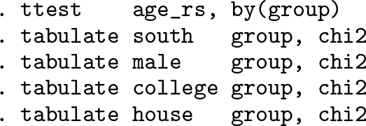
The second assumption—no liar—requires respondents in the longlist group to answer the key item truthfully. It is not statistically feasible to check this assumption, not only because respondents’ answers to the key item are by design unobserved but also because their truthful answers are unknown (otherwise there is no point in using the item-count technique).

The third assumption—no design effect—requires respondents not to change their answers to nonkey items depending on whether the key item appears in the list. Suppose that a respondent in the shortlist group answers one nonkey item affirmatively. If he or she were assigned to the longlist group, his or her answer must be either “one” or “two” (that is, he or she either answers one nonkey item affirmatively or answers one nonkey item plus the key item affirmatively). Blair and Imai (2012, 64) propose a statistical test for the no-design-effect assumption. 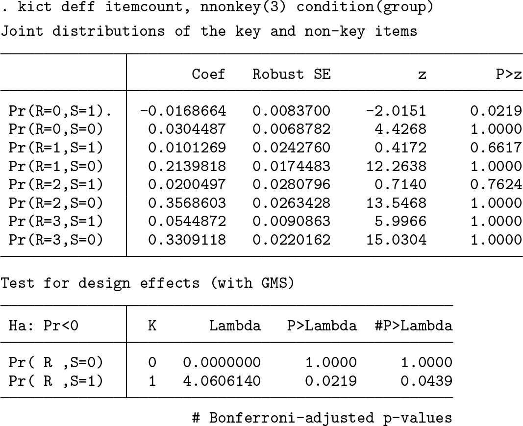kict deff implements that test and summarizes the results in two tables:

The first table lists estimated probabilities of all possible types of item-count responses. For example, Pr(R=0,S=1) estimates the joint probability of answering all nonkey items negatively and answering the key item affirmatively. This estimate is a nonsensical value (−0.02), raising doubts about the validity of the no-design-effect assumption. The next step is to check whether such a negative estimate has arisen by chance. The second table shows two hypothesis tests: one tests the null hypothesis that none of Pr(R=r,S=0) is smaller than zero; the other tests that none of Pr(R=r,S=1) is smaller than zero.⁵

When either of these tests is statistically significant, researchers should conclude that the no-design-effect assumption does not hold.⁶

The difference-in-means estimator

Let us assume for a moment that the 1991 American National Race and Politics Survey satisfies all three fundamental assumptions of the item-count technique. Then a basic analysis is to estimate the proportion of people who answer the key item affirmatively. kict ls with the option estimator(linear) can perform the difference-in-means estimation (1):

In this output, the central focus is Delta_cons. It means that 6.8% of white Americans would be upset by a black family moving in next door.⁷ As for Gamma_cons, it gives a predicted number of affirmative answers to the nonkey items—that is, white Americans, on average, feel angry over 2.1 nonkey items. This statistic is of no immediate interest to researchers, though it must be estimated simultaneously.

Note that, regardless of estimators, kict‘s output always uses Delta to label the coefficients that are directly related to the key item. The remaining coefficients in the output are labeled according to estimator developers’ notations to suit the convenience of interested readers for referring back to the formula in section 2 and in the literature. For space considerations, I concentrate on the Delta coefficients in the rest of this demonstration.

The linear least-squares estimator

Kuklinski, Cobb, and Gilens (1997) analyze whether whites in the Southern United States have a higher level of racial prejudice than other white Americans do. They answer this question by applying the differences-in-means estimator to the subsample of Southern whites and the other whites in the survey and then testing for the difference between two estimates.

Taking a more sophistic approach, Imai (2011, 412) estimates the regional difference in racial prejudice while controlling for other sociodemographic characteristics. The output below replicates his analysis by a linear least-squares regression [similar to (2)].⁸ The coefficient of interest is Delta_south, which is 0.20; this indicates that, ceteris paribus, racial prejudice is more prevalent among Southern whites than among other whites by 20 percentage points, but the difference does not reach statistical significance at the conventional level of 0.05.

One disadvantage of the linear least-squares estimation is unreasonable prediction. For example, a 21-year-old college-educated female non-Southern white’s probability of feeling anger over a black family moving in next door is estimated at −0.17(= 0.20×0+ 0.73×0.21+0.18×0+0.11×1−0.43). This is nonsensical because a probability cannot be a negative value. We can avoid this problem by using the nonlinear least-squares estimator.⁹

The nonlinear least-squares estimator

kict ls with the option estimator(nonlinear) performs nonlinear least-squares estimation [similar to (3)]. It uses a logistic function to restrict predicted values within the unit interval. Based on the output below,¹⁰ the 21-year-old college-educated female non-Southern white’s probability of feeling anger over a black family moving in next door is now estimated at a positive value: logit⁻¹(2.49×0+2.6×0.21+3.10×0+0.61×1−7.08) = 0.003.

Because of the logistic parameterization, Delta coefficients can be interpreted based on predicted values or odds ratios similarly to logistic regression coefficients. For example, Delta_south is 2.49, suggesting that, holding all other variables constant, Southern whites’ odds of being upset by a black family moving in next door are higher than the other whites’ odds by a factor of e ^2.49 (see Long [1997, 68–82]).¹¹

Imai’s maximum likelihood estimator

Imai’s maximum likelihood estimator (4) is an alternative to the nonlinear least-squares estimator. By default, kict ml with the option estimator(imai) implements this estimator using the following setups:

\begin{array}{l} S_{i} | X_{i} = x \overset{indep}{\sim} Bernoulli {{logit}^{- 1} (x^{'} δ)} \\ {logit}^{-}^{1} (x^{'} δ) = P (S_{i} = 1 | X_{i} = x) \\ R_{i} | S_{i} = s, X_{i} = x \overset{indep}{\sim} Binomial {J, l o g i t^{- 1} (x^{'} ψ_{s})} \\ {logit}^{-}^{1} (x^{'} ψ_{s}) = P (R_{i, j} = 1 | S_{i} = s, X_{i} = x) \end{array}

kict ml also produces a set of Delta coefficients that estimate the associations between respondents’ characteristics (X _i ) and their potential answers to the key item (S_i ). The interpretation of these coefficients is the same as explained previously because kict ml still uses the logistic function for parameterization. For example, Delta_age is 6.55, meaning that being one year older is expected to increase the odds of feeling angry over a black family moving in next door by a factor of e ^6.55×0.01. (Remember that the variable age is rescaled.)¹²

Furthermore, the Psi0 and Psi1 equations model respondents’ counts of affirmative answers to nonkey items (R_i ). These equations, though of no immediate interest to researchers, are crucial to the validity of the Delta coefficients. Note that kict ml by default assumes that R_i conditionally follows a binomial distribution. Substantively, this implies two additional assumptions: 1) (R_i,j ⊥ R_i,k )|S_i, X _i —each respondent’s answer to a nonkey item is independent of his or her answer to any other nonkey item; 2) P (R_i,j = 1|S_i, X _i ) = P (R_i,k = 1|S_i, X _i )—the probability that a respondent answers a nonkey item affirmatively is identical to the probability that he or she answers any other nonkey item affirmatively.

These assumptions do not always hold true. For example, a commonly used strategy to prevent respondents from answering all items affirmatively or negatively is to include an extremely low or high prevalent nonkey item into the list. This strategy jeopardizes assumption 2. Another strategy is to use negatively correlated nonkey items (Glynn 2013, 163). However, this risks violating assumption 1.

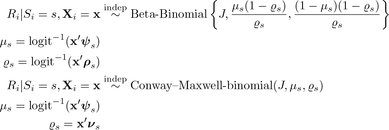
A way to relax these two assumptions is to use other distributions to model R_i . kict ml currently provides two alternative distributions: the beta-binomial distribution, which is particularly useful when nonkey items are positively correlated, and the Conway–Maxwell binomial distribution, which allows either a positive or negative correlation among nonkey items.¹³

\begin{array}{l} R_{i} | S_{i} = s, X_{i} = x \overset{indep}{\sim} Beta-Binomial {J, \frac{µ_{s} (1 - ϱ_{s})}{ϱ_{s}}, \frac{(1 - µ_{s}) (1 - ϱ_{s})}{ϱ_{s}}} \\ µ_{s} = {logit}^{-}^{1} (x^{'} ψ_{s}) \\ ϱ_{s} = {logit}^{-}^{1} (x^{'} ρ_{s}) \\ R_{i} | S_{i} = s, X_{i} = x \overset{indep}{\sim} Conway - Maxwell-binomial (J, µ_{s}, ϱ_{s}) \\ µ_{s} = {logit}^{-}^{1} (x^{'} ψ_{s}) \\ ϱ_{s} = x^{'} ν_{s} \end{array}

Nonetheless, both alternative distributions require kict ml to estimate additional coefficients, adding considerable complexity to optimization. Moreover, neither alternative guarantees to fit R_i well, especially when the relationships among nonkey items are highly complicated (for example, correlations vary from one pair of nonkey items to another, and the probability of answering an item affirmatively is different from that of another item). In fact, because respondents do not report their answers to each nonkey item, there is insufficient information to identify an appropriate distribution for R_i . This is an inherent limitation of the standard item-count technique. Some studies have attempted to address this limitation (for example, Corstange [2009]; Tsai [2018]), but more work is still needed.

Another significant aspect of Imai’s estimator is regarding the relationship between responses to the key and nonkey items. By default, kict ml uses the most flexible specification to model that relationship: the Psi0 coefficients are free to differ from their counterparts in the Psi1 equation. This specification, as illustrated by (10), not only allows R_i,j to be correlated with S_i but also allows the correlation to be moderated by X _i .¹⁴

P (R_{i, j} = 1 | S_{i}, X_{i}) = {logit}^{- 1} {ψ_{α}_{0} + X_{j}^{'} ψ_{β}_{0} + S_{i} (ψ_{α}_{1} - ψ_{α}_{0}) + {(S_{i} X_{i})}^{'} (ψ_{β}_{1} - ψ_{β}_{0})}

P (R_{i, j} = 1 | S_{i}, X_{i}) = {logit}^{- 1} {ψ_{α}_{0} + X_{i}^{'} ψ_{β}_{0}}

P (R_{i, j} = 1 | S_{i}, X_{i}) = {logit}^{- 1} {ψ_{α}_{0} + X_{i}^{'} ψ_{β}_{0} + S_{i} (ψ_{α}_{1} - ψ_{α}_{0})}

P (R_{i, j} = 1 | S_{i}, X_{i}) = {logit}^{- 1} {ψ_{α}_{0} + S_{i} (ψ_{α}_{1} - ψ_{α}_{0})}

P (R_{i, j} = 1 | S_{i}, X_{i}) = {logit}^{- 1} (ψ_{α}_{0})

Imai (2011, 412) proposes a simpler specification. He assumes that R_i,j and S_i are independent after controlling X _i and accordingly restricts all Psi0 coefficients to match their Psi1 counterparts (11). kict ml can perform this specification by imposing two constraints: [Psi0=Psi1] and [Psi0=Psi1]:_cons. There are other specifications. For example, (12) allows for a correlation between R_i,j and S_i while assuming no moderate effect of X _i (use the constraint [Psi0=Psi1]). Equation (13) assumes no correlation between R_i,j and X _i ([Psi0p=Psi1p], [Psi0p]:X1=0, [Psi0p]:X2=0,…). Equation (14) assumes that neither S_i nor X _i correlates with R_i,j ([Psi0p=Psi1p], [Psi0p=Psi1p]:_cons, [Psi0p]:X1=0, [Psi0p]:X2=0,…). All these specifications are nested in (10). The likelihood-ratio test is suitable for comparing and choosing among specifications.

Advanced issues for maximum likelihood estimators

Imai’s maximum likelihood estimator is complex and hence potentially difficult to optimize (so are the other maximum likelihood estimators demonstrated later). None of Stata’s built-in optimization algorithms guarantee finding the global maximum. A trick to handle this issue is to optimize a model from different random initial values. kict ml with the option protect( # ) does this trick. Many trials provide reasonable assurance that the result is not a local but a global maximum.

For example, the syntax below requires kict ml to perform 51 optimizations (each with 100 iterations at the most). Optimization 0 uses Stata’s default initial values; optimizations 1–50 use random-initial values. rseed() specifies the starting randomnumber seed. kict ml reports the result with the largest log-likelihood value among the trials, but users may add the option verbose to the syntax to monitor the result of every trial.

Furthermore, because of its complexity, Imai’s estimator is also prone to the problems of complete separation and boundary values. The quasi-Bayesian approach is a possible solution to these problems. Following Gelman et al. (2008), kict ml with the option pscale() uses independent Cauchy distributions as weakly informative priors, each centered at zero and with user-specified scales. Before fitting a model by this approach, Gelman et al. suggest centering and rescaling regressors in the first instance. In our example, that is,

The next step is to decide which coefficients need priors and how informative their priors should be. For illustrative purposes, I impose a prior with a scale parameter 2.5 on every slope coefficient in the Delta and Psi0 equations. For intercepts, I use a prior with a scale parameter 10. No prior is for the Psi1 coefficients because I intend to constrain them and their Psi0 counterparts to be equal. Accordingly, I generate a matrix of scale parameters, define two constraints, and fit the model by the quasi-Bayesian approach as follows:

No matter whether the quasi-Bayesian approach is adopted, kict ml always constructs CI for regression coefficients based on the assumption that the sampling distributions of the coefficient estimates are asymptotically normal. kict pfci is a postestimation command for producing CI based on the profile likelihood. The profile-based

CI does not rest on the normality assumption (Royston 2007) and is hence more robust than the normal-based CI when the sample size is small or when nonnormal priors are used.

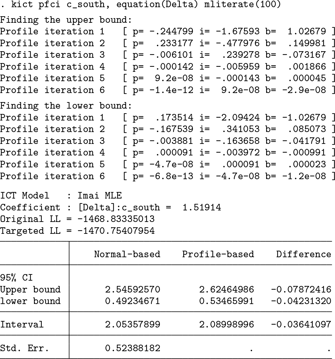
kict pfci works for one coefficient at a time. For example, the output below is specifically for coefficient c_South in equation Delta. The normal-based results are identical to those reported in the output of kict ml (shown previously). The calculation of the profile-based CI involves reoptimizing the model many times (the option mliterate(100) sets that each optimization perform a maximum of 100 iterations).

All the commands, options, and discussions above apply to the other maximum likelihood estimators demonstrated later in this section.

4.2 The partial item-count technique

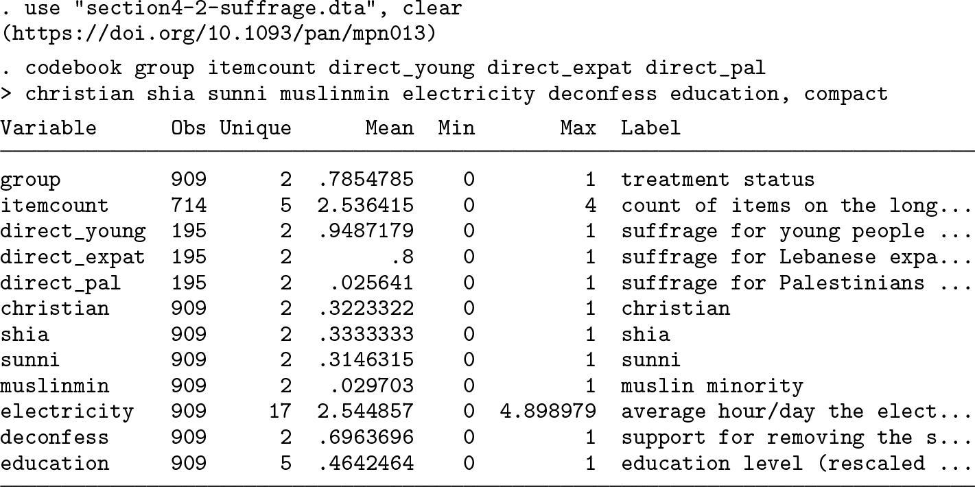
To gauge Lebanese attitudes toward voting rights for illiterates, Corstange (2009) uses the partial item-count technique in a Lebanese nationwide face-to-face survey. He requires a quarter of randomly selected respondents to answer each of the following items separately and directly:

“There has been some debate recently over who should have the right to vote in Lebanese elections. I’ll read you some different groups of people: please tell me if they should be allowed to vote or not.

Young people between the ages of 18 to 21;

Lebanese expatriates living abroad;

Palestinians without Lebanese citizenship.”

The rest of respondents answer to the question below in the item-count format, where the third item in the list is the key item:

“There has been some debate recently over who should have the right to vote in Lebanese elections. I’m going to read you the whole list, and then I want you to tell me how many of the different groups you think should be allowed to vote. Don’t tell me which ones, just tell me how many.

Young people between the ages of 18 to 21;

Lebanese expatriates living abroad;

Illiterate people;

Palestinians without Lebanese citizenship.”

After casewise deletion, the sample size for analysis is 909 (see the codebook output). The dataset contains an indicator variable (group) that takes on the value 0, representing the shortlist group, or 1, representing the longlist group. Because there are three nonkey items and a key item, the item-count response is a variable taking on integers from 0 to 4. The sample size of this variable is 714 because only the longlist group answers the item-count question. The sample size of the variables direct_young, direct_expat, and direct_pal is 195, because only the shortlist group answers these nonkey items in the direct questioning format.¹⁵ There are also variables for multivariate analysis. christian, shia, sunni, and muslinmin are four mutually exclusive binary variables representing respondents’ religions (the following example uses christian as the baseline category). electricity, deconfess, and education measure respondents’ material well-being, attitudes on fuller democratization, and levels of educational attainment, respectively (Corstange 2009, 58).

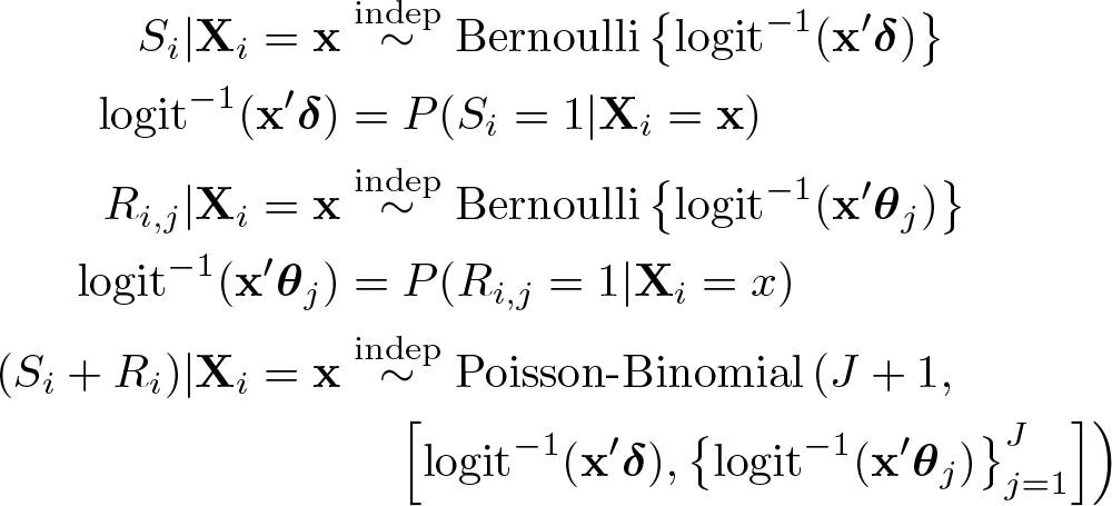
Corstange (2009) conducts an analysis by using a maximum likelihood estimator (6) that assumes that each respondent’s item count approximately follows a binomial distribution. kict ml with the estimator(corstange) and distribution(binomial) options performs that estimator with the following setups:

\begin{array}{l} S_{i} | X_{i} = x \overset{indep}{\sim} Bernoulli {{logit}^{- 1} (x^{'} δ)} \\ {logit}^{-}^{1} (x^{'} δ) = P (S_{i} = 1 | X_{i} = x) \\ R_{i, j} | X_{i} = x \overset{indep}{\sim} Bernoulli {{logit}^{- 1} (x^{'} θ_{j})} \\ {logit}^{-}^{1} (x^{'} θ_{j}) = P (R_{i, j} = 1 | X_{i} = x) \\ (S_{i} + R_{i}) | X_{i} = x \overset{indep}{\sim} Binomial (J + 1, π_{i}) \\ π_{i} {{logit}^{- 1} (x^{'} δ) + \sum_{j = 1}^{J} {logit}^{- 1} (x^{'} θ_{j})} / (J + 1) \end{array}

The output below replicates table 1 of Corstange (2009, 59). The Delta equation estimates the probability of supporting the enfranchisement of illiterates. The Theta equations from 1 to 3 estimate the probabilities of supporting the enfranchisement of three different groups described in nonkey items. Corstange does not use any variable to model the first and third nonkey items. This is equivalent to restricting slope coefficients in the Theta1 and Theta3 equations to be zero.

Blair and Imai (2012) improve Corstange’s estimator by using a Poisson-binomial distribution to model respondents’ item counts. kict ml with the estimator(corstange) and distribution(poisbino) options performs that modified estimator with the setups below. (The output is omitted because its arrangement and interpretation are the same as the previous.)

\begin{array}{l} S_{i} | X_{i} = x \overset{indep}{\sim} Bernoulli {{logit}^{- 1} (x^{'} δ)} \\ {logit}^{-}^{1} (x^{'} δ) = P (S_{i} = 1 | X_{i} = x) \\ R_{i, j} | X_{i} = x \overset{indep}{\sim} Bernoulli {{logit}^{- 1} (x^{'} θ_{j})} \\ {logit}^{-}^{1} (x^{'} θ_{j}) = P (R_{i, j} = 1 | X_{i} = x) \\ (S_{i} + R_{i}) | X_{i} = x \overset{indep}{\sim} Poisson-Binomial (J + 1, [1 {ogit}^{- 1} (x^{'} δ) + {1 {ogit}^{- 1} (x^{'} θ_{j})}_{j = 1}^{J}]) \end{array}

Blair and Imai’s estimator generally outperforms Corstange’s when the probability of answering an item in the affirmative varies greatly from one item to another. Nonetheless, note that both estimators assume that items are conditionally independent. It remains unclear about which estimator is more robust to the violation of that assumption.

4.3 Item-count techniques with auxiliary information

Eady (2017, 252–257) investigates Canadians’ attitudes toward gender equality through an Internet survey by using both the standard item-count technique and a direct question. A random half of respondents (the longlist group) are prompted with the following item-count question:

“How many of the following do you agree with?

There should be more funding for the arts

The government should raise taxes on gasoline

Corporations are taxed too much

Women are as competent as men in politics

Unions have too much power”

The other half of respondents (the shortlist group) are prompted by the same question without the sensitive item (the fourth one). Later in the same survey, all respondents are required to answer the sensitive question directly. In other words, those in the longlist group answer the key item twice:

“Do you agree or disagree with the following statement? ‘Women are as competent as men in politics.’ ”

The sample size for analysis is 22,372 (see the codebook output below). The dataset contains an item-count variable (itemcount) and a group indicator (group). A more noteworthy variable is direct_key, which recodes respondents’ answers to the direct question on the sensitive item. This variable provides auxiliary information for the itemcount estimation. There are also five variables for modeling the key item (ideology, gender, education, mothertongue, region).¹⁶

Aronow et al.’s (2015) difference-in-means estimator

Eady (2017) argues that, while respondents who deny gender equality may misreport their attitudes for avoiding social disapproval, those who agree with the norm should have no incentive to give a false answer. In this regard, Aronow et al.’s difference-inmeans estimator with the positive monotonicity assumption (8) is suitable to estimate the prevalence of the belief in gender equality in Canada. kict ls with the options auxiliary() and monotony(positive) can perform this estimation.

In the output above, Delta_cons is the estimated prevalence of the belief in gender equality. kict ls produces this estimate based on both the item-count variable itemcount and the auxiliary variable direct_key. The standard error (0.0113) is almost the same with that of the estimate based only on itemcount (0.0115—not displayed in the output). This suggests that direct_key does not provide sufficient information for a substantial reduction in estimation uncertainty.

Zeta_cons is the estimated prevalence of the belief in gender equality based only on direct_key. This estimate is often subject to the misreporting bias. In this example, Zeta_cons is higher than Delta_cons, suggesting that many people who deny gender equality misreport their attitudes. As for DeltaA0_cons, DeltaA1_cons, GammaA0_cons, and GammaA1_cons, these are the estimates of P (S_i = 1|A_i = 0), P (S_i = 1|A_i = 1), P (R_i = 0|A_i = 0), and P (R_i = 0|A_i = 1), respectively.

This difference-in-means estimator rests on two assumptions. First, A_i is independent of T_i . We may test this assumption with ttest direct_key, by(group). The second assumption is that A_i is monotonically related to S_i . If this assumption and the three fundamental assumptions for the item-count technique (footnote 3) all hold true, $\hat{P} (S_{i} = 1 | A_{i} = 0)$ must be close to 0 (Aronow et al. 2015, 8–9). Based on this idea, we can jointly test these four assumptions with test b[DeltaA0:_cons]=0.¹⁷

Eady–Tsai’s maximum likelihood estimator

Besides the overall prevalence of the belief in gender equality, Eady is also interested in whether that belief varies along ideological lines. He conducts a regression analysis using the maximum likelihood estimator shown in (9) (hereafter “Eady–Tsai’s estimator”). kict ml with the options estimator(tsaieady) and auxiliary() performs that estimator by the setups below:

\begin{array}{l} S_{i} | X_{i} = x \overset{indep}{\sim} Bernoulli {{logit}^{-}^{1} (x^{'} δ)} \\ {logit}^{- 1} (x^{'} δ) = P (S_{i} = 1 | X_{i} = x) \\ A_{i} | S_{i} = s, X_{i} = x \overset{indep}{\sim} Bernoulli {{logit}^{-}^{1} (x^{'} κ_{s})} \\ {logit}^{-}^{1} (x^{'} κ_{s}) = P (A_{i} = 1 | S_{i} = s, X_{i} = x) \\ R_{i} | A_{i} = a, S_{i} = s, X_{i} = x \overset{indep}{\sim} Binomial {J, l o g i t^{-}^{1} (x^{'} ψ_{s})} \\ {logit}^{- 1} (x^{'} ψ_{s}) = P (R_{i, j} = 1 | A_{i} = a, S_{i} = s, X_{i} = x) \end{array}

The option monotony() can be specified, if necessary, to impose the monotonicity assumption on P (A_i = 1|S_i = s, X _i = x).

The output below replicates the second model in table 4 of Eady (2017, 256). Two coefficients are particularly of interest. First, Delta_ideology suggests that the more politically left individuals are, the more likely they are to believe in gender equality. The standard error (0.032) is slightly smaller than that of the estimate without auxiliary information (0.041—not displayed in the output). Second, Kappa0_ideology suggests that, for those who deny gender equality, the more individuals are to the left politically, the more likely they are to misreport their belief [remember that the kappa0 equation represents $\hat{P} (A_{i} = 1 | S_{i} = 0, X_{i} = x)]$ .

Several technical points are noteworthy. First, the model above does not estimate the kappa1 equation because of the positive monotonicity assumption. (kappa1 is relating to $\hat{P} (A_{i} = 1 | S_{i} = 1, X_{i} = x)]$ , which is fixed at 1 in this example.)¹⁸ Second, Eady includes group into the kappa0 equation as a covariate to release the assumption that A_i and T_i are independent. Eady, however, does not include group into the other equations, so the model constrains the respect coefficients to be zero. Third, when monotony(positive) is specified, kict ml automatically drops A_i (direct_key) from the Psi1 equation to prevent perfect collinearity. Likewise, under the negative monotonicity assumption, A_i is dropped from the Psi0 equation. Fourth, kict ml by default assumes that R_i follows a binomial distribution (see Imai’s maximum likelihood estimator on page 411 for the implications of this assumption). Moreover, Eady assumes that R_i and S_i are correlated (that is, allowing Psi0_cons 6= Psi1_cons), but there is no moderate effect of X _i on that correlation (that is, restricting [Psi0=Psi1] for all slopes except those for group and direct_key).

4.4 The dual-list item-count technique

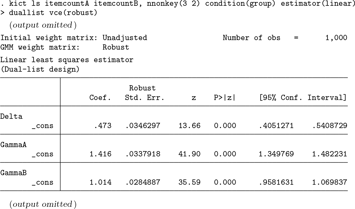
Consider the dual-list design presented in table 1: two item-count questions having the same key item but different nonkey items—three nonkey items for Q^A and two for Q^B . To demonstrate this design, I construct an artificial dataset as follows:

The output below demonstrates that each item-count variable is sufficient to produce an estimate of the population average response to the key item (Est_QA and Est_QB). The mean of these two estimates produces a more precise estimate: the standard error of Est_Dual is smaller. Note that the third and fourth lines in the nlcom syntax are the dual-list version of the difference-in-means estimator (5). (The first and second lines in the nlcom syntax are unnecessary if you are not interested in the separate estimates.)

kict ls with the options estimator(linear) and duallist is a shortcut to performing the dual-list version of the difference-in-means estimator, as demonstrated below. The numbers 3 and 2 in nnonkey() are the numbers of the nonkey items of itemcountA and itemcountB, respectively. Delta_cons in the output below is the same as Est_Dual shown above. GammaA_cons is the predicted number of affirmative answers to the nonkey items of Q^A , and GammaB_cons is the predicted number of affirmative answers to the nonkey items of Q^B .

kict ls can also help to conduct multivariate analysis for the dual-list design. For example, the following syntax performs linear and nonlinear least-squares regressions (15) to model the key item by three covariates, x1, x2, and x3:

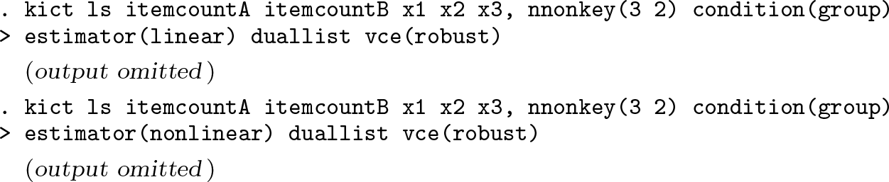
Regarding maximum likelihood estimation, kict lm with the options duallist and estimator(imai) performs the estimator derived in (16). The first part of the following syntax performs that estimator; the second and third parts of the syntax perform the single-list version of Imai’s maximum likelihood estimator for Q^A and Q^B , respectively. The variances of the Delta coefficients in IML_Dual are roughly half as large as those in IML_A and IML_B. This example clearly illustrates how the dual-list design can help to reduce estimation uncertainty.

4.5 The item-sum technique

To demonstrate the item-sum design illustrated in The item-sum technique on page 397, I construct an artificial dataset as follows:

kict ls with the options estimator(linear) and itemsum performs linear leastsquares estimation for the key item. In the artificial example, Delta_cons is 147.9, suggesting that the population average earnings from undeclared work is around e147.9 per month. Gamma_cons suggests that, on average, an individual’s monthly expenditure on housing plus weekly hours of TV watching is 516.4.

On multivariate analysis, the interpretation of the Delta coefficients is the same as the interpretation of the linear regression coefficients. Suppose that x2 is a variable of gender taking on the value 1 for men or 0 for women. Delta_x2 in the output below indicates that, ceteris paribus, men’s average monthly earnings from the undeclared work are e74.9 less than women’s.

5 Concluding remarks

In this article, I reviewed recent developments of the item-count technique and introduced a package, kict, for statistical analysis of item-count data. The review provides a general guide to the applications of the technique, and the package offers every convenience for data analysis. However, note that every item-count technique and their respective statistical methods rest on certain assumptions and have their own limitations. Although I gave an overview of those issues, applied researchers should still refer to and familiarize themselves with the relevant literature to avoid any misuse.

The kict package has provided many commonly used methods for researchers to analyze several popular types of item-count data. Undeniably, there are methods that have not been built in kict, especially those that are overly individualized such as the estimators with corrections for certain bias (for example, Blair and Imai [2012, 66–68]; Blair, Chou, and Imai [2018]). Those estimators are difficult to program because their formulas are highly contingent upon individual researchers’ assumptions about the bias to be corrected. Of course, I could have programmed those estimators based on one or two assumptions, but the resulting commands would have been severely limited and of little practical use. Abuse is also a matter of concern because careless users may misperceive those commands as “one-size-fits-all” corrections. I decided to postpone programming overly individualized methods but will resume doing it after formulating an appropriate strategy for programming.

The development of the item-count technique is still ongoing. There are more and more interesting variant designs and new methods for data analysis (for example, Chaudhuri and Christofides [2013, 115–150]; Blair, Imai, and Lyall [2014]; Chou, Imai, and Rosenfeld [Forthcoming]; Ibrahim [2016]; Tsai [2018]). I will continue to update the kict package accordingly.

Supplemental Material

Supplemental Material, st0559 - Statistical analysis of the item-count technique using Stata

Supplemental Material, st0559 for Statistical analysis of the item-count technique using Stata by Chi-lin Tsai in The Stata Journal

Footnotes

Notes

Appendix

I first modify Imai’s least-squares estimators [(2) and (3)] to accommodate to the duallist design of the item-count technique. I continue to use the notations introduced in The dual-list item-count technique on page 394 and additionally define $R_{i, j}^{A}$ and $R_{i, j}^{B}$ as respondent i’s potential answers to the jth and kth nonkey items of Q^A and Q^B , respectively, where j = 1,…, J, and k = 1,…, K. Accordingly, the respondent’s answers to Q^A and Q^B are $Y_{i}^{A} = R_{i}^{A} + T_{i} S_{i}$ _i and $Y_{i}^{B} = R_{i}^{B} + (1 - T_{i}) S_{i}$ , respectively, where $R_{i}^{A} = \sum_{k = 1}^{K} R_{i, k}^{B}$ . Moreover, let $Y_{i}^{L} = T_{i} Y_{i}^{A} + (1 - T_{i}) Y_{i}^{B}$ consider the following simultaneous equation model for analyzing the dual-list item-count data:

NOTES:

g(X i, δ ) = E(S_i |X _i) = P (S_i = 1|X _i).

f(X i, γA) = E(RiA|X _i).

h(X i, γB) = E(RiB|X _i).

Additional assumptions: $E (\in_{i}^{A} | X_{i}, T_{i}) = 0$ and $E (\in_{i}^{B} | X_{i}, T_{i}) = 0$ .

In the linear least-squares estimation, g(·), f(·), and h(·) are identity-link functions. For nonlinear estimation, kict ls defines g(X _i, δ ) = logit⁻¹(x ^′ δ ), f(X _i, γ ^A ) = J logit⁻¹(x ^′ γ ^A ), and h(X _i, γ ^B ) = K logit⁻¹(x ^′ γ ^B ). Conceptually, the coefficients are estimated through the following three-step procedure:

Computationally, kict ls converts these steps into moment conditions and uses the generalized method of moments (gmm) for estimation (see also Drukker [2014]; Imai [2011, 415]).

Second, I attempt to modify Imai’s maximum likelihood estimator (4) for the dual-list item-count technique. Equation (16) shows the likelihood function of one possible modification:

NOTES:

1 _Condition = 1 if Condition holds; 1 _Condition = 0 otherwise.

Additional assumptions: the distributions of RiA and RiB.

Third, I apply Eady and Tsai’s idea about auxiliary information to Corstange’s partial item-count technique. Equation (17) is the likelihood function:

\begin{array}{l} \prod_{i \in (T_{i} = 0)} {\prod_{j = 1}^{J} P (R_{i, j} = r_{j} | A_{i} = a, X_{i} = x, θ_{j}) \\ \times \sum_{s = 0}^{1} P (A_{i} = a | S_{i} = s, X_{i} = x, κ_{s}) P (S_{i} = s | X_{i} = x)} \\ \times \prod_{i \in (T_{i} = 1)} \sum_{s = 0}^{1} {{(1_{Y_{i} \neq J + 1})}^{1 - s} {(1_{y_{_{i} \neq 0}})}^{s} \\ \times {\sum_{u \in U^{Y_{i} - s}} \prod_{j = 1}^{J} P (R_{i, j} = r_{u, j} | A_{i} = a, X_{i} = x, θ_{j}) \\ \times P (A_{i} = a | S_{i} = s, X_{i} = x, κ_{s}) P (S_{i} = s | X_{i} = x, δ) \end{array}

NOTES:

1 _Condition = 1 if Condition holds; 1 _Condition = 0 otherwise.

U^Y_i−s is a set of combinations of R_i,j that satisfy R_i = Y_i − s.

u is one of the combinations in U ^Y_i−s.

r_u,j = 1 if R_i,j = 1 in u; r_u,j = 0 otherwise.

Additional assumptions:

A_i is independent of T_i .

A_i is predictive of S_i .

A_i is extraneous to S_i .

S_i , R_i,j , and R_i,k (j ≠ k) are independent after controlling for X _i.

References

Andrews

D. W. K.

Soares

2010. Inference for parameters defined by moment inequalities using generalized moment selection. Econometrica 78: 119–157.

Aronow

P. M.

Coppock

Crawford

F. W.

Green

D. P.

2015. Combining list experiment and direct question estimates of sensitive behavior prevalence. Journal of Survey Statistics and Methodology 3: 43–66.

Blair

Chou

Imai

2018. List experiments with measurement error. Technical report. Princeton University. https://imai.fas.harvard.edu/research/files/listerror.pdf.

Blair

Imai

2012. Statistical analysis of list experiments. Political Analysis 20: 47–77.

Blair

Imai

Lyall

2014. Comparing and combining list and endorsement experiments: Evidence from Afghanistan. American Journal of Political Science 58: 1043–1063.

Chaudhuri

Christofides

T. C.

2013. Indirect Questioning in Sample Surveys. Berlin: Springer.

Chou

Imai

Rosenfeld

Forthcoming. Sensitive survey questions with auxiliary information. Sociological Methods and Research.

Corstange

2009. Sensitive questions, truthful answers? Modeling the list experiment with LISTIT. Political Analysis 17: 45–63.

Droitcour

Caspar

R. A.

Hubbard

M. L.

Parsley

T. L.

Visscher

Ezzati

T. M.

1991. The item count technique as a method of indirect questioning: A review of its development and a case study application. In Measurement Errors in Surveys, ed. Biemer

P. P.

Groves

R. M.

Lyberg

L. E.

Mathiowetz

N. A.

Sudman

, 185–210. Hoboken, NJ: Wiley.

10.

Drukker

2014. Using gmm to solve two-step estimation problems. The Stata Blog: Not Elsewhere Classified. http://blog.stata.com/2014/12/08/using-gmm-to-solve-two-step-estimation-problems/.

11.

Eady

2017. The statistical analysis of misreporting on sensitive survey questions. Political Analysis 25: 241–259.

12.

Gelman

2014. Thinking of doing a list experiment? Here’s a list of reasons why you should think again. Statistical Modeling, Causal Inference, and Social Science. https://andrewgelman.com/2014/04/23/thinking-list-experiment-heres-listreasons-think/.

13.

Gelman

Jakulin

Pittau

M. G.

Y.-S.

2008. A weakly informative default prior distribution for logistic and other regression models. Annals of Applied Statistics 2: 1360–1383.

14.

Glynn

A. N.

2013. What can we learn with statistical truth serum? Design and analysis of the list experiment. Public Opinion Quarterly 77: 159–172.

15.

Holbrook

A. L.

Krosnick

J. A.

2010. Social desirability bias in voter turnout reports: Tests using the item count technique. Public Opinion Quarterly 74: 37–67.

16.

Ibrahim

2016. An alternative modified item count technique in sampling survey. International Journal of Statistics and Applications 6: 177–187.

17.

Imai

2011. Multivariate regression analysis for the item count technique. Journal of the American Statistical Association 106: 407–416.

18.

Jann

2005. rrlogit: Stata module to estimate logistic regression for randomized response data. Statistical Software Components S456203, Department of Economics, Boston College. https://ideas.repec.org/c/boc/bocode/s456203.html.

19.

Kadane

J. B.

2016. Sums of possibly associated Bernoulli variables: The Conway– Maxwell-binomial distribution. Bayesian Analysis 11: 403–420.

20.

Kudo

1963. A multivariate analogue of the one-sided test. Biometrika 50: 403–418.

21.

Kuklinski

J. H.

Cobb

M. D.

Gilens

1997. Racial attitudes and the “new south”. Journal of Politics 59: 323–349.

22.

Long

J. S.

1997. Regression Models for Categorical and Limited Dependent Variables. Thousand Oaks, CA: Sage.

23.

Royston

2007. Profile likelihood for estimation and confidence intervals. Stata Journal 7: 376–387.

24.

Sniderman

P. M.

Tetlock

P. E.

Piazza

1991. Data of 1991 race and politics survey. Survey Research Centre, University of California, Berkeley. http://sda.berkeley.edu/cgi-bin/hsda?harcsda+natlrace.

25.

Trappmann

Krumpal

Kirchner

Jann

2014. Item Sum: A New Technique for Asking Quantitative Sensitive Questions. Journal of Survey Statistics and Methodology 2: 58–77.

26.

Tsai

C.-l.

2017. Solutions to turnout over-reporting: What is out there, what works, and can we do better? Doctoral dissertation, University of Essex.

27.

Tsai

C.-l.

2018. “A random-wording design for improving the item-count technique”. Paper presented at the 2018 Annual Meeting of the American Political Science, August 30–September 2, 2018, Boston, MA.

28.

Von Hermanni

2016. “List experiment: Past and present”. Paper presented at the Conference of European Statistics Stakeholders, October 20–21, 2016, Budapest, Hungary.

29.

Wolter

Laier

2014. The effectiveness of the item count technique in eliciting valid answers to sensitive questions. An evaluation in the context of self-reported delinquency. Survey Research Methods 8: 153–168.

Supplementary Material

Please find the following supplemental material available below.

For Open Access articles published under a Creative Commons License, all supplemental material carries the same license as the article it is associated with.

For non-Open Access articles published, all supplemental material carries a non-exclusive license, and permission requests for re-use of supplemental material or any part of supplemental material shall be sent directly to the copyright owner as specified in the copyright notice associated with the article.

0.25 MB

0.00 MB