In this article, we present a new command, xtspj, that corrects for incidental parameter bias in panel-data models with fixed effects. The correction removes the first-order bias term of the maximum likelihood estimate using the split-panel jackknife method. Two variants are implemented: the jackknifed maximum-likelihood estimate and the jackknifed log-likelihood function (with corresponding maximizer). The model may be nonlinear or dynamic, and the covariates may be predetermined instead of strictly exogenous. xtspj implements the split-panel jackknife for fixed-effects versions of linear, probit, logit, Poisson, exponential, gamma, Weibull, and negbin2 regressions. It also accommodates other models if the user specifies the log-likelihood function (and, possibly but not necessarily, the score function and the Hessian). xtspj is fast and memory efficient, and it allows large datasets. The data may be unbalanced. xtspj can also be used to compute uncorrected maximum-likelihood estimates of fixed-effects models for which no other xt (see [XT] xt) command exists.
Panel-data analysis is an important tool in economic studies. In many panel-data applications, each cross-sectional unit or “individual” is allowed to have a latent unit-specific characteristic, or individual effect, that may be correlated with the covariates and hence must be controlled for. A standard tool to control for unobserved individual effects in panel data is the fixed-effects model, in which a separate parameter, or fixed effect, is included for each of the N individuals in the dataset. Recent empirical studies using fixed-effects models are, for example, Egger and Staub (2016), Griffin and Maturana (2016), and Milner et al. (2016). However, it is well known that the presence of fixed effects may introduce bias into the maximum likelihood (ML) estimator of the common parameters (the parameters assumed to be shared by all individuals, such as regression coefficients) when the number of time periods, T , is small. Specifically, the large-N, fixed-T probability limit of the ML estimator may be inconsistent. This is known as the incidental parameter problem (IPP) of Neyman and Scott (1948). Lancaster (2000) provides a survey on the IPP. Some models that are subject to the IPP are the probit model (for example, Fernández-Val [2009]), the logit model (for example, Katz [2001]), and the tobit model (for example, Greene [2004]). But even in the linear model with fixed effects, there is an IPP for the slope coefficients unless the regressors are strictly exogenous (Chudik, Pesaran, and Yang 2018).
To describe the IPP, let us consider an outcome variable Yit, where i = 1,…, N and t = 1,…, T . Suppose Yit, given Xit, has a density function f(Yit|Xit; θ, αi), where θ is the common parameter vector, αi is the scalar fixed-effects parameter associated with the ith individual, and Xit is a vector of observed covariates. The ML estimator of αi is to be obtained only from T observations. Therefore, when T is fixed, remains random even as N → ∞. This randomness enters the log likelihood and, in many models, causes the ML estimator of θ to converge to an incorrect probability limit , where θ0 is the true value of θ. For a fixed T , no consistent alternative estimator of θ0 can generally be found because θ0 may not be point identified; see, for example, Honoré and Tamer (2006) and Chamberlain (2010). When both N, T → ∞, the randomness in αbi vanishes and converges to θ0 in general. However, when N/T converges to a positive constant as N, T → ∞, the asymptotic distribution of is often not centered at zero, invalidating inference and confidence intervals based on standard ML theory; see, for example, Hahn and Kuersteiner (2002) and Hahn and Newey (2004).
Researchers have been attempting to find solutions to the IPP. For instance, Cox and Reid (1987), Woutersen (2001), and Lancaster (2002) show that a parameter transformation that orthogonalizes θ and the αi may help to resolve the IPP or at least mitigate it. Andersen (1970) and Chamberlain (1980) show that in certain models, the maximizer of a conditional likelihood function, given sufficient statistics for the αi, is a large-N, fixed-T consistent estimator; the logit model is a well-known example. However, these methods are not general, because there is no guarantee that, in a given model, an orthogonalizing parameter transformation exists nor that a conditional likelihood exists.
In search for methods that apply more generally, researchers have been trying to correct for the bias of caused by the fixed effects. These methods are approximate in nature. The idea is to remove the first-order term of a large-T approximation of the bias of . Hahn and Newey (2004) and Hahn and Kuersteiner (2011) develop formulas of the first-order bias of . This formula, evaluated at ML estimates of θ and the αi, is subtracted from to give a first-order bias-corrected estimate, that is, an estimate with first-order bias equal to zero. Fernández-Val and Weidner (2016) provide the first-order bias formula for the case where both individual effects and time effects are present. Alternatively, the log-likelihood function or, equivalently, the score function may be treated as the object that has to be bias corrected. For instance, Arellano and Bonhomme (2009) and Arellano and Hahn (2016) discuss first-order modified log-likelihood functions as an alternative to the usual log-likelihood function. Maximization of a modified log-likelihood function gives a first-order bias-corrected estimate. Li, Lindsay, and Waterman (2003) consider first-order modified score functions. Solving a modified score equation leads to a first-order bias-corrected estimate.
Approximate bias corrections can also be carried out without explicit bias formulas, for example, by using the jackknife. The jackknife is due to Quenouille (1949, 1956). In the context of the IPP, Hahn and Newey (2004) introduce the delete-one panel jackknife for first-order bias correction in static panel models. For dynamic models, Dhaene and Jochmans (2015) propose the split-panel jackknife (SPJ). The panel is split into two half-panels along the time dimension, and ML is applied to each half-panel separately, giving and , say. The SPJ estimate, then, is defined as and is a first-order bias-corrected estimate of θ. The same procedure can also be applied to the (concentrated) log likelihood to give a jackknifed log likelihood, whose maximizer is a first-order bias-corrected estimate of θ.
In this article, we implement the SPJ in Stata. Our new command, xtspj, takes as input a log likelihood written in terms of one or more linear indices (equations in the Stata language), either user-specified or preprogrammed. xtspj currently comes with preprogrammed fixed-effects log likelihoods of the (Gaussian) linear, probit, logit, Poisson, exponential, gamma, Weibull, and negbin2 regression models. The covariates are allowed to contain lagged values of the dependent variable. Hence, autoregressive versions of these models can be fit without user input. As main output, xtspj produces the SPJ estimates (in one of the two possible variants) or, if desired, the uncorrected ML estimates. The maximization routine used by xtspj exploits the sparsity of the Hessian of the log likelihood, so it is fast and memory efficient.
xtspj allows the panel dataset to be unbalanced. As discussed in Dhaene and Jochmans (2015), the jackknifed log-likelihood variant of the SPJ naturally allows for unbalanced data, so xtspj implements this variant as described there. It is less straightforward to define the jackknifed estimator variant for unbalanced data. xtspj defines and implements this variant via an estimator that is close to the ML estimator: the weighted average of the ML estimates associated with the balanced panel components that jointly form the full (unbalanced) panel, with weights taken in proportion to the balanced panel component sample sizes. Each of the balanced panel estimates can be jackknifed separately, and the resulting estimates can be averaged using the same weights. We conduct a simulation study of this variant of the SPJ when the data are unbalanced, showing that it works well. It should be mentioned that Chudik, Pesaran, and Yang (2018) introduce another variant of the SPJ for unbalanced data. They split the full (unbalanced) panel into two unbalanced half-panels such that the observations for each cross-sectional unit i are equally split over the two half-panels, and then form the SPJ estimate in the same way as in the balanced case.
xtspj is a complementary tool to the commands probitfe and logitfe recently developed by Cruz-Gonzalez, Fernández-Val, and Weidner (2017). These commands implement analytical and jackknife bias corrections—including the SPJ—for common parameter and average marginal effect estimates in probit and logit models with individual effects, time effects, or both. In comparison, xtspj implements the SPJ for the common parameters in models with individual effects only (if desired, time effects can be included as common parameters). On the other hand, xtspj is set up for a more general class of models, including user-written models. xtspj is also faster and can handle very large datasets.
This article is organized as follows. Section 2 introduces the use of xtspj together with the preprogrammed models and presents the syntax, output, and examples. Section 3 discusses the extension of the SPJ to deal with unbalanced data. Section 4 presents simulation results for unbalanced data. Section 5 provides details on how to use xtspj with a user-written model; the probit model serves as an example. Section 6 discusses details of the algorithms underlying xtspj. Section 7 concludes. Three appendixes contain technical details and the source code for the evaluation of the preprogrammed log likelihoods. The full source code of the preprogrammed log likelihoods, the code for the simulations, and additional simulation results are available in an online supplement available at https://www.researchgate.net/publication/328837218.
2 The command: Basics
This section presents the basic syntax and use of xtspj. For xtspj with user-written models, see section 5. Importantly, xtspj also computes the uncorrected ML estimate, so it may as well be used for fast and memory-efficient computation of ML estimates of fixed-effects models for which a suitable xt (see [XT] xt) command does not exist.
First, recall the definition of the SPJ for balanced data (see section 3 for unbalanced data). Consider a panel dataset of observations Yit with i = 1,…, N indexing the individuals and t = 1,…, T indexing time, and suppose T is even (see Dhaene and Jochmans [2015] for the case with T odd). Let be the ML estimate of θ computed from the full panel, and let and be the ML estimates computed from, respectively, the first half-panel, where t = 1,…, T/2, and the second half-panel, where t = T/2 + 1,…, T . The SPJ estimator is defined as
The SPJ log likelihood is defined similarly. Let be the concentrated log-likelihood function computed from the full panel (by concentrating out the αi), and let and be the concentrated log-likelihood functions computed from, respectively, the first and the second half-panels. Then, the SPJ log likelihood is
and the corresponding jackknife estimator is
Both and are first-order bias-corrected estimators. For a comparison of the two variants, Dhaene and Jochmans (2015) provide extensive discussion and simulations.
xtspj implements the first-order SPJ (also termed the half-panel jackknife) for possibly nonlinear models with fixed effects. xtspj accepts balanced and unbalanced datasets, with one restriction: for every cross-sectional unit i, there must be no gaps in the time series. Hence, missing data are allowed only at the beginning and end of the observation period. depvar is the regressand in the model, and indepvars is an optional list of regressors that may contain lagged values of depvar. The data must be xtset (see [XT] xtset) with both panelvar and timevar. xtspj accepts fvvarlist (see [U] 11.4.3 Factor variables) (for example, i.x) and tsvarlist (see [U] 11.4.4 Time-series varlists) (for example, L.x) in indepvars but not in depvar. Prior to estimation, the indepvars are checked for multicollinearity. When indepvars contains lagged values of depvar up to p lags, the model becomes autoregressive of order p and is fit conditionally on the first p observations. The current version of xtspj maximizes the objective function using the Newton–Raphson algorithm.
2.3 Options
model(string) specifies the type of regression model to be fit: probit (probit), logit (logit), linear (linear), negative binomial (negbin), Poisson (poisson), exponential (exponential), gamma (gamma), Weibull (weibull), or some other user-written model. For user-written models, see section 5. The linear model can also be fit by specifying model(regress); see section 2.5. model() is required.
method(string) takes none, like, or parm for, respectively, no correction (), the SPJ based on the jackknifed log likelihood (), and the SPJ based on the jackknifed estimator (). method() is required.
level(#) sets the confidence level. The default is level(95).
ltol(#) sets the tolerance level for changes in the objective function value. When the difference between the objective function values in the current and the previous iteration, divided by the absolute value of the current objective function value, is nonnegative and less than ltol(#), the algorithm stops and reports that convergence has been achieved. The default is ltol(1e-4).
ptol(#) sets the tolerance level for changes in the parameter values. The algorithm stops and reports convergence when the change in the parameter is less than ptol(#). The change is computed as the absolute difference between θ in the current and the previous iteration. When θ is a vector, the maximum element of the vector of absolute differences is taken. The default is ptol(1e-4).
maxiter(#) sets the maximum number of iterations the algorithm is allowed to use. The default is maxiter(100).
diagnosis specifies that a simple diagnostic algorithm be invoked when the Newton– Raphson algorithm gives an updated parameter vector that does not improve the objective function value. This diagnostic algorithm is slow and disabled by default. Our recommendation is to activate diagnosis (together with verbose) in case of nonconvergence problems.
verbose specifies whether the iteration log of the maximization (that is, the objective function values) and extra notes (for example, about omitted individuals) should be displayed on the screen. When method(parm) is requested, the iteration log can be lengthy. It is disabled by default.
alpha(newvar) specifies the name of the variable to be created, if needed, to store the estimates αbi of the fixed effects αi (the same value for all T observations corresponding to i). When method(none) is requested, is the ML estimate of αi. When method(like) or method(parm) is requested, is the ML estimate of αi with θ held fixed in the likelihood function at or , respectively.
2.4 Stored results
xtspj stores the following in e():
2.5 Remarks
The covariance matrix of the estimated θ is computed as follows. When no correction is requested (method(none)), the usual oim covariance matrix based on the Hessian of the concentrated log likelihood is computed—see [R] vce_option. When method(like) or method(parm) is requested, the covariance matrix is obtained from the same Hessian but now evaluated at the corresponding estimate, or . This requires maximizing the uncorrected log likelihood with respect to the fixed-effects parameters while θ is kept fixed at or . For this maximization, the options ltol(), ptol(), and maxiter() are also effective.
When diagnosis is turned on, a diagnostic algorithm is invoked every time the current objective function value in the Newton–Raphson algorithm is less than that in the previous iteration (see also Baldick [2006, 403]). Given the gradient vector and Hessian matrix obtained from the previous iteration, the algorithm successively reduces the step size, used to update the parameter vector, from 1 to 0.5, 0.5^2,…, possibly down to a minimum value of 0.5^10. The objective function is evaluated at the parameter vector updated with the reduced step size. When the objective function value improves on that from the previous iteration, the diagnostic algorithm stops, and maximization continues from the currently updated parameter vector. Otherwise, the step size is further reduced unless the minimum step size is already reached, in which case the diagnostic algorithm reports that no improvement could be achieved by reducing the step size, the algorithm stops, and maximization continues from the parameter vector obtained before the diagnostic algorithm was called.
With regard to ereturn, e(ll) is a stored result only when method(none) or method(like) is requested.
The standard behavior of xtspj is to compute the estimates using the Newton–Raphson algorithm to maximize the associated objective functions. This also applies to model(linear). However, for the linear model, the ML and the two jackknife estimates are also available in closed form. For the ML and jackknifed ML estimates, this is straightforward: ML is just ordinary least squares, and the jackknifed ML estimate is just a linear combination of ordinary least-squares estimates. For the jackknife estimate based on the jackknifed log likelihood, , the closed-form expression (accommodating unbalanced data) is derived in appendix A. As an alternative to model(linear), model(regress) computes the estimates in the linear model directly from the closed-form expressions and therefore is much faster.
For the probit and logit models, a check is performed for each individual i in each of the half-panels to ensure that Yit varies across t. This is to drop individuals for whom the regressand is perfectly predicted by setting αi equal to −∞ or +∞. These individuals are not informative about θ in the corresponding half-panel and are excluded from the estimation altogether. A similar check is performed in, for example, probit (see [R] probit). Similarly, for the Poisson and negative binomial regression models, individuals for which the regressand is zero for all t are uninformative and are therefore dropped. For the exponential, gamma, and Weibull regression models, individuals for which the regressand is nonpositive are dropped, similarly to streg (see [ST] streg).
2.6 Example
To illustrate xtspj, we use a synthetic dataset on whether workers complain to managers at fast-food restaurants. The data setup is as follows:
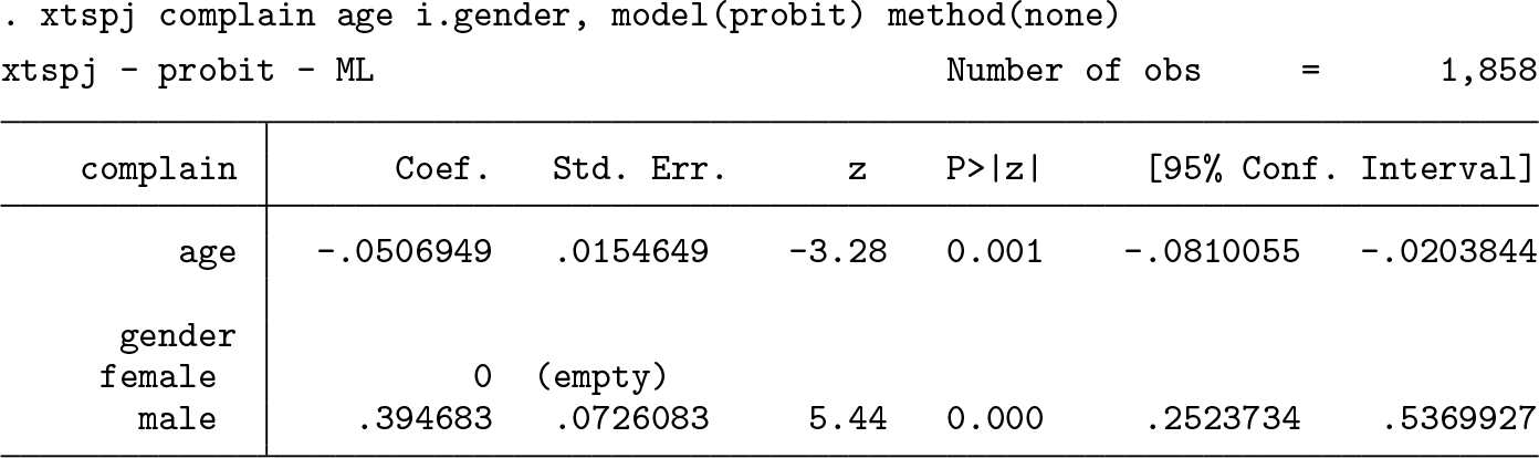
Uncorrected fixed-effects probit ML
The model is specified with fvvarlist (see [U] 11.4.3 Factor variables) in the list of regressors, the output table is standard, and i0. gender, with value female, is omitted because of multicollinearity. The omitted variable is listed in the output table but is assigned a zero coefficient. Number of obs reports the effective number of cross-sectional and time-series observations used in the estimation, after excluding uninformative individuals (restaurants, in this example). When the option verbose is specified, the list of excluded individuals and the list of omitted regressors are reported. The title of the table, xtspj – probit – ML, lists the name of the command, the name of the model, and the estimation method.
Jackknifed log likelihood
Number of obs is much smaller here because any individual i is kept only if it is informative in each of the subpanels used to form the jackknife estimate. Hence, individuals that are informative in the full panel but not in one or more subpanels are excluded. Likewise, the multicollinearity check is performed at the level of each subpanel and, hence, it may occur that additional regressors have to be omitted (relative to ML) because they do not pass the multicollinearity check in each subpanel. Clearly, when the number of observations or the list of regressors is different between the ML and the jackknife estimates, it becomes harder to compare the estimates.
Jackknifed ML
Number of obs and the set of omitted regressors are the same as for method(like). This is because method(like) and method(parm) use the same multicollinearity and informativeness checks. The estimates, however, are different.
3 Unbalanced panels and the SPJ
3.1 Unbalanced panels and the ML estimator
For simplicity of the analysis of unbalanced data, it is assumed that missingness is at random and that every individual i contributes only consecutive data (that is, there are no gaps). Then, an unbalanced panel can always be viewed as the union of J balanced panels, indexed by j = 1,…, J. The jth balanced panel has Nj individuals, each with Tj consecutive periods of data. Consider now an asymptotic setup where Nj, Tj → ∞ and Nj/Tj → κj with 0 < κj < ∞ for all j, and let J be fixed. First, the ML estimator obtained from the unbalanced panel is briefly studied, and a closely related estimator is suggested that can easily be jackknifed.
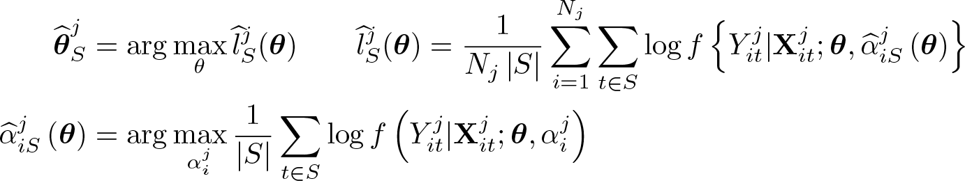
For the (i, t)th observation of the jth balanced panel, denote the outcome variable as and the regressors as . The conditional density of , given , is , where is the fixed-effects parameter. Let
The jth log likelihood, , is normalized by the number of observations in the jth balanced panel, so . The log likelihood corresponding to the full (that is, unbalanced) panel, normalized by the number of observations, is
where wj = NjTj/∑j NjTj is the weight of the jth balanced panel. Hence, the ML estimator is
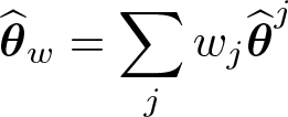
Consider the weighted average of the ,
and call it the weighted-average ML estimator. The ML and weighted-average ML estimators are closely related, as the expressions show. It may be conjectured that they are asymptotically equivalent under weak conditions. We will not study the precise conditions here, because they are not the focus of this article. We will, however, conduct a small-scale simulation study in section 4, showing that and are close to each other. Our proposal is to jackknife by jackknifing , as discussed below in section 3.2.
As an example, the remainder of this subsection examines the many-normal-means IPP of Neyman and Scott (1948) under data unbalancedness. The observations Yit follow the normal distribution N (αi, θ0), with common variance θ0 and different means αi; there are no covariates. When the panel is balanced, the (normalized) log-likelihood function is
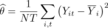
Plugging in for αi gives the concentrated log likelihood,
and, on maximizing,
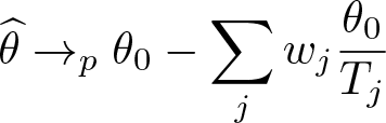
It follows easily that, as N → ∞ with T fixed,
that is, is inconsistent and biased toward zero. All of this has been well known since Neyman and Scott (1948).
Now consider the unbalanced case. For the jth balanced panel, the concentrated log likelihood and its maximizer are
where is the ML estimator of . The concentrated log likelihood for the full panel is
with maximizer
Thus, the ML estimator, , and the weighted-average ML estimator, , are identical. Furthermore, when Nj → ∞ and Tj is fixed for all j,
When Tj → ∞ for all j,
Even when J is allowed to grow with the sample size, will typically be consistent because
where ∑jNj/∑jNjTj → 0 under weak conditions on the sequences (Nj, Tj), j = 1,…,J, as J grows. For the asymptotic distribution of to be centered at 0, it can easily be shown that
is necessary and sufficient. When the panel is balanced, that is, J = 1, N1 = N, and T1 = T , (1) is equivalent to N/T = o(1), which is well known as necessary and sufficient for to be centered at 0; see, for example, Hahn and Newey (2004).
3.2 Unbalanced panels and the SPJ
Our proposal is to jackknife by jackknifing the closely related estimator . Given that is a weighted average of ML estimates defined by balanced panels, can be jackknifed by parts, that is, by jackknifing each in the usual way and then forming a weighted average of the jackknifed using weights wj.
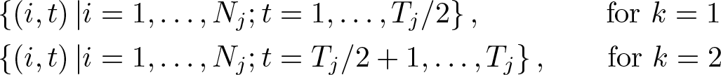
Consider panel j. To allow Tj to be even or odd, we need to introduce a little more notation. When Tj is even, the jackknife splits panel j into two subpanels with Tj/2 time periods each. Let
The SPJ computes, for
where |S| = Tj/2 denotes the number of elements in S. Letting and for k = 1, 2, the jackknifed versions of and are, as before,
When Tj is odd, the situation is slightly different because there are two ways of splitting panel j into almost equal subpanels. Let
where ⌈Tj/2⌉ is the least integer τ satisfying τ ≥ Tj/2 and ⌊Tj/2⌋ is the greatest integer τ satisfying τ ≤ Tj/2. (Note that and when Tj is even.) The jackknifed versions of and are then defined as
The estimator is new, while was proposed in Dhaene and Jochmans (2015). The two estimators, and , remove the leading bias term of and , respectively. They are consistent, have the same large-N, large-T asymptotic variance as and , and their limit distributions are correctly centered. That is, under our asymptotic setup, with denoting the total number of observations, the limit distributions of and are normal and centered at zero, while those of and are normal but not generally centered at zero.
As mentioned in the introduction, Chudik, Pesaran, and Yang (2018) propose an alternative splitting scheme for unbalanced panels. We give a brief comparison here. For simplicity, suppose Tj is even for all j = 1,…, J. The SPJ estimate of Chudik, Pesaran, and Yang (2018) is
where is the usual ML estimate computed from the full panel and is the ML estimate computed from the kth unbalanced half-panel, with observations
The estimator replaces with and with . The latter is a weighted average, over j, of the ML estimate computed from the kth half of the jth balanced panel, with observations
An advantage of is that it does not rely on the conjectured asymptotic equivalence of and , while does. On the other hand, Chudik, Pesaran, and Yang (2018) showed the bias-reduction property of in the unbalanced case only for dynamic linear models, whereas and are generally bias reducing in nonlinear models as well (relative to w and , respectively).
3.3 Practical considerations
For some panels j, Tj may be too small for or l˙j(θ) to be defined. In that case, the individuals in those panels have to be excluded from the estimation. xtspj checks only if Tj ≥ 2. This is a necessary condition for splitting the panel. All individuals with fewer than two periods of data are automatically excluded. When Tj = 2, the half-panel will contain only one time period, which in most models is insufficient to estimate θ. For example, the linear fixed-effects model requires at least two time periods in each subpanel, so the theoretical minimum for Tj is 4. Because this is a model-specific issue, the user must determine if Tj is large enough, and, if it is not, the user must exclude the corresponding individuals from the estimation, similarly to the ::Check() function discussed below in section 5.3. Furthermore, one may also choose to set the minimum for Tj above the theoretical minimum for at least two reasons. First, the panels with small Tj typically contribute more higher-order bias to the SPJ than those with greater Tj. Therefore, excluding panels with small Tj often reduces the bias but at the expense of increased variance. Second, for panels with very small Tj, the half-panel concentrated log likelihoods may be nearly flat, potentially causing numerical problems for computing the jackknife estimates.
xtspj does not allow gaps in the data. In particular, for every individual, missing data are allowed only at the beginning of the observation period, at the end, or both at the beginning and the end. In certain situations, this is a realistic assumption, but it is often unrealistic. However, this assumption is without loss of generality when the observations are assumed to be independent across time (conditional on covariates) because then we may simply reassign the observations to different time periods. For dynamic models, the situation is more complicated, and the assumption of consecutive data was primarily made to accommodate dynamic models without difficulty in the analysis. When the model is dynamic and there are gaps in the data, a simple solution (though with loss of efficiency) is to redefine an “individual” as a patch of consecutive observations. For example, an individual i with two patches of consecutive observations, separated by a gap, is replaced by two new individuals, one for each patch. Then, the analysis proceeds as in the case with consecutive data. The efficiency loss of this solution is twofold: more fixed effects have to be estimated, and more initial observations are lost because of conditioning on them. Avoiding the efficiency loss appears difficult in general, although in linear time-series models it may be possible to extend Wincek and Reinsel (1986) to the SPJ.
4 Simulations for unbalanced panels
This section presents a simulation study of the effect of moderate data unbalancedness on the performance of the SPJ. The results are based on 5,000 Monte Carlo replications. We set N = 500 throughout. The code used for the simulations is available in the online supplement.
We first present simulation results suggesting that, for unbalanced data, and are asymptotically equivalent (note that they are identical for balanced data). We simulated data from the probit model, Yit = 1(Xitθ0 + αi + εit ≥ 0), where εit ∼ N (0, 1), with θ0 = 0.5 and (Xit, αi) as specified below. We first generated balanced panels with T = 8,…, 18 and then introduced unbalancedness by letting a fraction r > 0 of the individuals have T − 4 observations instead of T . For example, when T = 8 and r = 0.25, the unbalanced panel consists of J = 2 balanced panels, one with N1 = 125 and T1 = 4, and the other with N2 = 375 and T2 = 8. We generated unbalanced panels with r = 0.25, 0.5, 0.75 (for balanced panels, r = 0). The covariate was generated as Xit ∼ N (αi, 1), with αi = 0 (design 1) or αi ∼ N (0, 1/2) (design 2). Design 1 is the case where, in fact, pooled estimation (that is, without fixed effects) is consistent, while design 2 calls for fixed-effects estimation because the αi are correlated with the regressor. Figures 1 and 2 present the bias and root mean squared error (RMSE) of and in the unbalanced designs.1 The first point to note is that there is an IPP even when there are no fixed effects (design 1). That is, fitting a fixed-effects model already induces an IPP even when the true data-generating process has no individual effects. In both designs, and are close to each other and so are their biases and RMSEs. The differences are most pronounced when T ≤ 10 and r = 0.5, and in those cases, tends to perform slightly better than in terms of RMSE. As T increases, the difference disappears as expected.
ML and weighted-average ML: probit model, design 1. Model: Yit = 1(Xitθ0 + αi + εit ≥ 0), εit ∼ N (0, 1). Data generated with θ0 = 0.5, Xit ∼ N (αi, 1), αi = 0 (design 1), N = 500, T on x axis, and rN individuals with T − 4 instead of T . ML = , weighted ML = .
ML and weighted-average ML: probit model, design 2. Model: Yit = 1(Xitθ0 + αi + εit ≥ 0), εit ∼ N (0, 1). Data generated with θ0 = 0.5, Xit ∼ N (αi, 1), αi ∼ N (0, 1/2) (design 2), N = 500, T on x axis, and rN individuals with T − 4 instead of T . ML = , weighted .
Next, we study the effect of data unbalancedness on the ML estimate, , and on the SPJ estimates, and . We consider three models: the static probit, the static logit, and the stationary Gaussian first-order autoregressive [AR(1)] model. We set T = 4,…, 18 in the balanced panels, which serve as a benchmark of comparison with unbalanced panels. For T ≥ 8, we generated unbalanced panels as above, with r = 0.25, 0.5, 0.75.
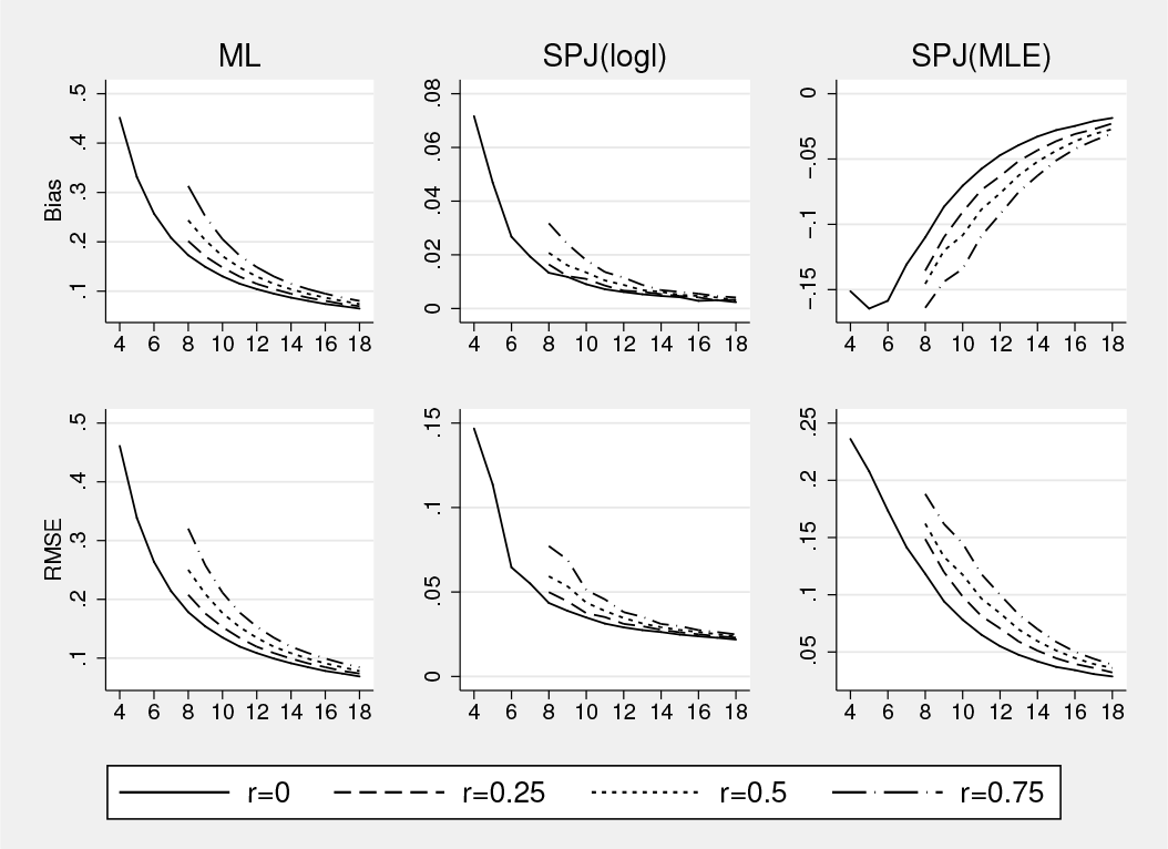
Figures 3–6 present the results for θ0 = 0.5, 1. The bias of the ML estimator is uniformly upward both in design 1 and design 2. Both variants of the jackknife yield significant improvements over ML in terms of bias and RMSE. The variant based on the jackknifed log likelihood tends to perform best. The bias of is uniformly downward in the designs studied, and the bias of is uniformly upward. Although this seems to suggest a general pattern, the pattern found here is specific to the chosen design. The effect of data unbalancedness shows a clear picture. For any T , as r increases from 0 to 0.75, an increasing fraction of the panel has only T − 4 observations, and the incidental parameter bias of all three estimators increases, as expected. Note further that T with r = 0 is equivalent to T + 4 with r = 1, so one can see the gradual effect of successively adding 4 time periods of data for a rotating group of 125 individuals from a balanced panel with T = 4 up to one with T = 18. In line with the theory, the bias changes smoothly for all three estimators in most design points and shows that the jackknife is also bias reducing for unbalanced data.
ML and SPJ: probit model, θ0 = 0.5, design 1. Model: Yit = 1(Xitθ0+αi+εit ≥ 0), εit ∼ N (0, 1). Data generated with θ0 = 0.5, Xit ∼ N (αi, 1), αi = 0 (design 1), N = 500, T on x axis, and rN individuals with T −4 instead of T . , SPJ(logl) = , SPJ(MLE) = . Maximum likelihood estimation = MLE.
ML and SPJ: probit model, θ0 = 0.5, design 2. Model: Yit = 1(Xitθ0+αi+εit ≥ 0), εit ∼ N (0, 1). Data generated with θ0 = 0.5, Xit ∼ N (αi, 1), αi ∼ N (0, 1/2) (design 2), N = 500, T on x axis, and rN individuals with T − 4 instead of T . ML = , SPJ(logl) = , SPJ(MLE) = .
ML and SPJ: probit model, θ0 = 1, design 1. Model: Yit = 1(Xitθ0 +αi +εit ≥ 0), εit ∼ N (0, 1). Data generated with θ0 = 1, Xit ∼ N (αi, 1), αi = 0 (design 1), N = 500, T on x axis, and rN individuals with T −4 instead of T . ML = , SPJ(logl) = , SPJ(MLE) = .
ML and SPJ: probit model, θ0 = 1, design 2. Model: Yit = 1(Xitθ0 +αi +εit ≥ 0), εit ∼ N (0, 1). Data generated with θ0 = 1, Xit ∼ N (αi, 1), αi ∼ N (0, 1/2) (design 2), N = 500, T on x axis, and rN individuals with T − 4 instead of T . ML = , SPJ(logl) = , SPJ(MLE) = .
For the static logit model, the data were generated as in the probit model above, except that here εit is standard logistically distributed and, in accordance with the scale of εit, the covariate was generated as Xit ∼ N (αi, π2/3), with αi = 0 (design 1) or αi ∼ N (0, π2/6) (design 2). The results for the logit model are available in the online supplement. They are similar to those for the probit model: is upward biased; and are far less biased and have smaller RMSE; the bias of all three estimators hanges smoothly with the degree of data unbalancedness; the jackknife is bias reducing for unbalanced data; and, again, the jackknife based on the jackknifed log likelihood performs best.
Figures 7–8 report the results for the stationary Gaussian AR(1) model, with data generated as
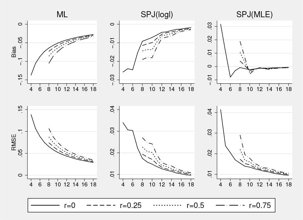
ML and SPJ: Gaussian AR(1) model, θ0 = 0.5, design 2. Model: Yit = θ0Yit−1 + αi + εit, εit ∼ N (0, 1). Data generated with θ0 = 0.5, stationary Yi0, αi ∼ N (0, 1/2) (design 2), N = 500, T on x axis, and rN individuals with T − 4 instead of T . ML = , SPJ(logl) = , SPJ(MLE) = .
ML and SPJ: Gaussian AR(1) model, θ0 = −0.5, design 2. Model: Yit = θ0Yit−1 + αi + εit, εit ∼ N (0, 1). Data generated with θ0 = −0.5, stationary Yi0, αi ∼ N (0, 1/2) (design 2), N = 500, T on x axis, and rN individuals with T −4 instead of T . ML = , SPJ(logl) = , SPJ(MLE) = .
where εit ~ N (0, 1), αi ~ N (0, 1/2) (design 2), and θ0 = 0.5, −0.5. The simulation results are qualitatively similar to those in the logit and probit models. Here, however, the jackknifed estimator, , performs better than in terms of bias and RMSE. This is in line with the simulation results in Dhaene and Jochmans (2015). Furthermore, the bias is not symmetric in θ0 around 0, in line with the analysis of Nickell (1981). The corresponding results for the case αi = 0 (design 1) are available in the online supplement. Apart from Monte Carlo error, these results are identical to those for design 2, confirming that all three estimators are invariant with respect to the αi.
To conclude, the simulation results confirm that can be jackknifed by jackknifing . The biases of are roughly equal to the corresponding weighted averages, using weights wj, of the biases associated with estimates computed from balanced panels. For example, when T1 = 6 and T2 = 10, the bias of θ˙ is roughly the weighted average of the bias when T = 6 and the bias when T = 10. The bottom line is that, at least for moderately unbalanced panels, data unbalancedness poses no problem for the SPJ.
5 User-written models
xtspj can also be used with a user-written model, provided that the density function is of the form
with
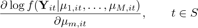
for an arbitrary number M ≥ 1 of linear indices µm,it (equations in the Stata language) depending on covariates Xm,it. The regressand, Yit, can be a vector, at most of dimension M. The first linear index, µ1,it, contains an additive fixed effect. Nevertheless, this design is general in that when the fixed effects enter nonadditively, one simply needs to keep the first linear index free of covariates. One can also set Xm,it = 1 for one or several m > 1; then the corresponding µm,it = θm are simply parameters, entering the model as specified by f.
5.1 Syntax
5.2 Description
The rules for xtspj with a user-written model are the same as in section 2 with two exceptions. First, each eq (equation) specifies a linear index, µm,it. The specification of an eq is similar to ml model (see [R] ml), that is,
where eqname is an optional equation name, depvar and indepvars are specified as usual, and noconstant is optional and specifies that the corresponding equation has no constant term. Here the equal sign (=) is compulsory, even if the equation is completely empty in other parts of the specification; that is, eq must be, in the simplest form, (=). In the first eq, which is always without constant term because of the presence of fixed effects, noconstant is implicitly assumed without specifying it. When a factor variable appears among the indepvars in more than one eq, it must appear with a different name in each eq. Hence, one has to generate a duplicate of the variable underlying the factor variable for each additional eq where the factor variable appears. Second, model(string) contains the name of the user-written model, which has to be programmed according to the rules given below in section 5.3. The ereturn stored results are also as in section 2 except that e(depvar) now is the list of regressands.
5.3 User-written log-likelihood evaluation
The function f in (2) has to be specified as a Mata class containing two member functions, ::Evaluate() and ::Check() (see [M-2] class). As examples, the Mata classes for the preprogrammed models are given in appendix B, and the do-files are available in the online supplement. The template for the Mata class is as follows.
The user needs to supply the relevant Mata code in the lines 8 and 12 as discussed below and change “<YourModel>” (lines 2, 5, 10) to a desired name, for example, “MyModel”. When xtspj is executed, this name must be specified in the option model(string), for example, model(MyModel), so that xtspj calls the communitycontributed specification of f.
void function ::Evaluate()
The function ::Evaluate() needs to be supplied (see [M-2] declarations). It computes the model’s log likelihood, gradient, and Hessian for a given set of observations (i, t), tS.∈ S. The function is called repeatedly and separately for each i and various sets In balanced panels with even T , for example, S is {1,…, T } or {1,…, T/2} or {T/2 + 1,…, T }. The arguments of ::Evaluate() are as follows:
real matrix Y, the matrix of regressands. The kth column of Y corresponds to the kth regressand, defined by an eq, and each row corresponds to an observation (i, t), t ∈ S.
real matrix XB, the matrix of linear indices. The mth column of XB corresponds to the mth linear index, defined by an eq, and each row corresponds to an observation (i, t), t ∈ S.
real colvector LogLikelihood, the column vector of log-likelihood values. Each row contains the log-likelihood value corresponding to an observation (i, t), t ∈ S, evaluated at the corresponding row of XB and Y. Thus, LogLikelihood has elements
real matrix Gradient, the matrix of scores. The mth column of Gradient corresponds to the log-likelihood derivative with respect to the mth linear index, evaluated at XB and Y. Thus, the mth column of Gradient has elements
pointer(real colvector) matrix Hessian, the pointer matrix pointing to the Hessian (see [M-2] pointers). It must be symmetric (see [M-5] makesymmetric( )). The (m, n)th element of Hessian is a pointer to the column vector of second-order log-likelihood derivatives with respect to the mth and nth linear indices, evaluated at XB and Y. Thus, the (m, n)th element of Hessian points to the elements
The arguments real matrix Gradient and pointer(real colvector) matrix Hessian are optional. If they are not changed inside ::Evaluate(), xtspj uses a numerical differentiation algorithm to compute the derivatives. See section 6.1 for details.
The following Mata code gives ::Evaluate() for the probit model:
Compare code block 1 with the corresponding portion of the template code block: “probit” replaces “<YourModel>”, and LogLikelihood, Gradient, and Hessian are computed in lines 5 to 7. Lines 6 and 7 can be omitted; then Gradient and Hessian are computed by numerical differentiation.
Mata function arguments are passed by reference (see [M-2] declarations, remark 8), so the changes made inside the function-to-function arguments remain also after the function execution has terminated. Hence, the values computed and stored in LogLikelihood, Gradient, and Hessian are preserved after the function call and are passed to xtspj.
When a model contains more than one equation (M > 1), the variables Gradient and Hessian may be preallocated to reduce the computation time. This can be done by inserting the code
between lines 3 and 4 of code block 1 (see [M-5] J( ), [M-5] rows( ), and remark 8 of [M-2] pointers for NULL).
Hessian is computed as a matrix of pointers. In line 7 of code block 1, the operator &() creates a pointer to the value of the expression in parentheses, that is, a pointer to the value of -Gradient:*(XB+Gradient). There is a subtle difference between a pointer to a variable and a pointer to the value of an expression (see [M-2] pointers, remarks 2 and 3). When pointing to a variable, this may cause mistakes when that variable is reused. For example, the code
will not produce the intended result, because line 3 alters H and thus also Hessian[1,1]. It is on the safe side to use different variable names instead, as in
void function ::Check()
Prior to estimation, xtspj checks that for each individual, there are at least two time periods of data so that, when the panel is split, each subpanel has at least one time period per individual. Individuals that do not meet this condition are excluded from the estimation. The function ::Check() serves as an additional, model-specific data check and, if necessary, serves to additionally exclude individuals that are uninformative about θ in some subpanel or subpanels. For example, in the linear model, at least two time periods are required in each subpanel. Another example is that, in binary choice models, Yit must vary across t in each subpanel. If such data checks are not needed, one may simply replace line 12 of the template code block with “Keep=1”.
The function ::Check() is called prior to estimation and checks a given set of observations (i, t), t ∈ S. Similar to ::Evaluate(), ::Check() is called separately for each i and various sets S that correspond to the subpanels. Only if i passes the data check imposed by ::Check() for all relevant sets S (which results in “Keep=1” for all S) is i included in the dataset to be used for estimation. The arguments of ::Check() are as follows:
real matrix Data, the data to be checked. The columns of Data correspond to the regressands of the model, followed by the regressors, in the same order as specified by the equations. The rows correspond to the observations (i, t), t ∈ S.
real scalar Keep, the main output. Keep is set to 1 if Data passes the check and set to 0 otherwise.
The following Mata code gives ::Check() for the probit model:
Here line 2 tests if Y, the first column of Data, varies. When the elements of Y are all 0 or all 1, the expression
is evaluated as true and Keep is set to 0 (see [M-5] sum( ) and [M-2] op_logical). Otherwise, Y varies and Keep is set to 1.
5.4 Example
Here we compute the jackknifed ML estimate with the user-written model PROBIT, specified in the Mata part, for the same setup as in section 2.6. Note that the model name, PROBIT, is capitalized so that it does not conflict with the preprogrammed model named probit. The output table is identical to the corresponding output table in section 2.6 except for the model name, PROBIT.
6 Algorithms
6.1 Details on numerical differentiation
Numerical differentiation is a well-established technique for the approximation of the derivatives of a function when analytical differentiation is difficult or infeasible. The subject is treated extensively in, for example, Burden, Faires, and Burden (2016), Griewank and Walther (2008), and Press et al. (2007, chap. 5.7). In Mata, [M-5] deriv( ) computes numerical derivatives. However, xtspj does not use [M-5] deriv( ), because it is not optimized for the present setup. To see why, we briefly review the algorithm implemented by [M-5] deriv( ) and the implied time cost. Consider a generic log-likelihood function
where θ is a scalar common parameter and α = (α1,…, αN )′ is the vector of fixedeffects parameters. [M-5] deriv( ) approximates the first derivative of L(θ, α1,…, αN ),
as
for some small h. This is the standard formula discussed in many textbooks, including those cited above. (Higher-order techniques also exist; see, for example, Fornberg [1988].) Now, assuming the time cost of evaluating L(θ, α) is O(1), the time cost of approximating (3) as above is O(2N + 2) or, when θ is a vector of P elements, O(2N + 2P ). That is, it takes 2(N + P ) times as much time to compute the first derivative as to compute the value of the log-likelihood function. When the second derivative is approximated in the same way, the time cost becomes even much higher. In typical microeconomic panel datasets, N is large and T is small, so this algorithm is computationally very slow.
xtspj implements an alternative algorithm for numerical differentiation, exploiting the property that the model may be expressed in terms of linear indices. Given (2), the log-likelihood function may be written as
where µm is the NT × 1 vector collecting all the elements µm,it. Correspondingly, let Xm be the NT × Pm matrix collecting all the values of the regressors that appear in the mth linear index. Observing that
for every m, we have
Here we only have to approximateas
which requires just two evaluations of the log-likelihood function. For the fixed-effects parameter αi, we have
which is linked to objects already computed because
For the second derivative, a similar computation follows easily.
The algorithm just described is efficient in that the time cost is only slightly higher than O(2M), so the time spent obtaining the first derivative is roughly the same as that of evaluating the log-likelihood function 2M times. In typical settings, M is much less than N + P . For example, in the probit model, M = 1. In the linear model, M = 2 (there is a constant linear index for the error variance, say, In addition, for some models, the time cost of evaluating the derivatives analytically exceeds the time cost of computing them numerically using the proposed algorithm.
xtspj currently sets h equal to epsilon(1) ^ 0.25, where epsilon(1) is the machine precision (see [M-5] epsilon( )).
6.2 Details on the Newton–Raphson algorithm
The Newton–Raphson algorithm is a common technique for numerical optimization of functions that are twice differentiable. Its properties, potential problems, and implementation details can be found in, for example, Süli and Mayers (2003, chap. 4), Bonnans et al. (2006, chap. 4), and Press et al. (2007, chap. 9). In Stata and Mata, ml, optimize(), and moptimize()(see [R] ml, [M-5] optimize( ), and [M-5] moptimize( )) are numerical optimizers. In the context of ML estimation of fixed-effects models, the problem with these optimizers, including the standard way of implementing the Newton– Raphson algorithm, is that they do not exploit the sparsity of the Hessian matrix, which makes them slow and memory inefficient. This section reviews these problems and discusses how xtspj implements the Newton–Raphson algorithm more efficiently.
Consider first how one may fit a fixed-effects model by ML in Stata when no xt command is available. As an example, suppose one wishes to fit a fixed-effects probit model, given a panel dataset with a binary regressand Y, a regressor X, and a group variable i indexing the individuals (i is the panelvar in xtset). Then, one would run
This code is conveniently short but can be slow. As an example, we ran it with Stata/MP2 15.1 on an Intel i7-6820HQ computer for balanced datasets generated with Xit, αi ∼ N (0, 1), T = 10, θ0 = 0.5, and various values of N. As shown in table 1, the time cost of probit grows rapidly with N, while that of xtspj is roughly proportional to N.
Time cost of probit versus xtspj
Time using probit
Time using xtspj
N
Mean
Max
Mean
Max
10
0.03
0.05
0.04
0.06
100
0.15
0.17
0.06
0.08
500
4.26
4.51
0.16
0.18
1000
32.95
33.83
0.29
0.32
2000
277.03
281.55
0.51
0.54
NOTES: Time is reported in seconds. Mean and max are obtained by running probit and xtspj 10 times on the same dataset, generated with Xit and αi drawn from N (0, 1), T = 10, and θ0 = 0.5.
The number of parameters in fixed-effects models is N + dim θ, so when N is large, standard optimization methods become very slow. The SPJ adds to the challenge because the model has to be fit several times or, in the case of the jackknifed log likelihood, one has to optimize simultaneously over several sets of fixed-effects parameters. The number of fixed-effects parameters that implicitly enter l˙(θ) varies between 3N (when Tj is even for all i) and 5N (when Tj is odd for all i). In short, when N is large, the optimization problem is high dimensional. Standard optimizers that use second derivatives, such as the Newton–Raphson algorithm, become slow in high dimensions because the Hessian is high dimensional. Here, however, the Hessian is also sparse. In particular, the matrix of second derivatives of the original (unconcentrated) log likelihood with respect to all fixed-effects parameters is a diagonal matrix. This is also true, as shown in appendix C, for the Hessian of the unconcentrated objective function underlying l˙(θ), which depends on multiple sets of fixed-effects parameters. The sparsity of the Hessian simplifies its inversion and the updating step of the Newton–Raphson algorithm, as detailed below.
Let θ be a P × 1 column vector, and consider an objective function of the form
where wj is the weight associated with the jth balanced panel and α, γ, and δ are vectors of fixed-effects parameters associated with, respectively, all time periods, the first half, and the second half of the time periods (assuming Tj is even for all j). Partition the gradient and the Hessian as
Given the parameter vector (θ(k)′, ϕ(k)′)′ at the kth iteration, the Newton–Raphson algorithm obtains the updated parameter vector as
where
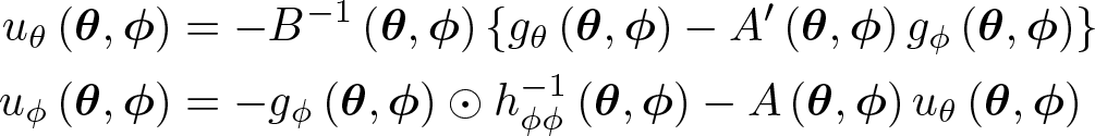
When dim ϕ is large, computing u(θ, ϕ) by Gaussian elimination is slow and inaccurate. As suggested by Hall (1978) and Chamberlain (1980), the computation of u(θ, ϕ) can be carried out more efficiently using a block inversion algorithm. Because Hφφ(θ, ϕ) is diagonal, only its diagonal needs to be stored, and it is straightforward and fast to compute
where ⊙ denotes the Hadamard product, 1P is the P × 1 vector of ones, and diag(V) is the column vector formed by the diagonal elements of V. Then
is given by
This way of computing the updated parameter vector is memory efficient and dramatically speeds up the Newton–Raphson algorithm.
7 Conclusion
xtspj implements the SPJ of Dhaene and Jochmans (2015) in Stata using code written in Mata. The command allows for unbalanced panels. It implements two variants of the SPJ: the jackknifed ML estimator and the jackknifed (concentrated) log likelihood. The model is generically defined through linear indices. The log-likelihood gradient and Hessian may be supplied by the user or computed numerically by xtspj. The command is much faster than standard Stata code because it is written in Mata and the maximization of the log likelihood is carried out by a tailored Newton–Raphson algorithm that exploits the sparsity of the Hessian.
The current version of xtspj is preliminary in several respects. For instance, unlike other Stata routines such as optimize(), moptimize(), and ml, xtspj does not support the Nelder–Mead algorithm (see, for example, Dennis and Woods [1987]) and does not allow constraints in the maximization. Further, xtspj provides a bias correction for fixed effects but not for time dummies (although the model may include time effects, treated as common parameters). Recently, Fernández-Val and Weidner (2016) extended the SPJ to models with both fixed and time effects, in an asymptotic setting where N/T converges to a positive constant. Also, xtspj is restricted to first-order bias correction, whereas higher-order versions of the SPJ exist as well (see Dhaene and Jochmans [2015]). Finally, xtspj focuses on estimating θ—the common parameter. There are, however, many other estimands of interest, for example, average marginal (or partial) effects or other average quantities that depend on θ, the fixed effects, and the covariate values. The ML estimates of such quantities are also biased because of the estimation of the fixed effects and may be bias corrected by the SPJ.
In applied work with panel data, most panel datasets are unbalanced. On the other hand, most theoretical work on panel data assumes balanced data. Here a version of the SPJ for unbalanced data is proposed, and its properties are investigated. We find that mild degrees of data unbalancedness pose no problem for the SPJ. The properties of the estimators under more extreme forms of data unbalancedness, for example, when the vast majority of individuals have only a few data periods remain to be investigated.
Supplemental Material
Supplemental Material, st0557 - xtspj: A command for split-panel jackknife estimation
Supplemental Material, st0557 for xtspj: A command for split-panel jackknife estimation by Yutao Sun and Geert Dhaene in The Stata Journal
Footnotes
8 Acknowledgments
We are grateful to a referee for valuable comments and suggestions. Financial support from the Flemish Science Foundation grant G.0505.11 and from the Fundamental Research Funds for the Central Universities (grant 2412018QD026) are gratefully acknowledged.
Notes
References
1.
AndersenE. B.1970. Asymptotic properties of conditional maximum-likelihood estimators. Journal of the Royal Statistical Society, Series B32: 283–301.
2.
ArellanoM.BonhommeS.2009. Robust priors in nonlinear panel data models. Econometrica77: 489–536.
3.
ArellanoM.HahnJ.2016. A likelihood-based approximate solution to the incidental parameter problem in dynamic nonlinear models with multiple effects. Global Economic Review45: 251–274.
4.
BaldickR.2006. Applied Optimization: Formulation and Algorithms for Engineering Systems. Cambridge: Cambridge University Press.
5.
BonnansJ.-F.GilbertJ. C.LemaréchalC.SagastizábalC. A.2006. Numerical Optimization: Theoretical and Practical Aspects. 2nd ed. New York: Springer.
ChamberlainG.1980. Analysis of covariance with qualitative data. Review of Economic Studies47: 225–238.
8.
ChamberlainG.. 2010. Binary response models for panel data: Identification and information. Econometrica78: 159–168.
9.
ChudikA.PesaranM. H.YangJ.-C.2018. Half-panel jackknife fixed-effects estimation of linear panels with weakly exogenous regressors. Journal of Applied Econometrics33: 816–836.
10.
CoxD. R.ReidN.1987. Parameter orthogonality and approximate conditional inference. Journal of the Royal Statistical Society, Series B49: 1–39.
11.
Cruz-GonzalezM.Fernández-ValI.WeidnerM.2017. Bias corrections for probit and logit models with two-way fixed effects. Stata Journal17: 517–545.
12.
DennisJ. E.Jr.WoodsD. J.1987. Optimization on microcomputers: The Nelder-Mead simplex algorithm. In New Computing Environments: Microcomputers in Large-Scale Computing, ed. WoukA., 116–122. Philadelphia: Society for Industrial and Applied Mathematics.
13.
DhaeneG.JochmansK.2015. Split-panel jackknife estimation of fixed-effect models. Review of Economic Studies82: 991–1030.
14.
EggerP. H.StaubK. E.2016. GLM estimation of trade gravity models with fixed effects. Empirical Economics50: 137–175.
15.
Fernández-ValI.2009. Fixed effects estimation of structural parameters and marginal effects in panel probit models. Journal of Econometrics150: 71–85.
16.
Fernández-ValI.WeidnerM.2016. Individual and time effects in nonlinear panel models with large N, T. Journal of Econometrics192: 291–312.
17.
FornbergB.1988. Generation of finite difference formulas on arbitrarily spaced grids. Mathematics of Computation51: 699–706.
18.
GreeneW.2004. Fixed effects and bias due to the incidental parameters problem in the tobit model. Econometric Reviews23: 125–147.
19.
GriewankA.WaltherA.2008. Evaluating Derivatives: Principles and Techniques of Algorithmic Differentiation. 2nd ed. Philadelphia: Society for Industrial and Applied Mathematics.
20.
GriffinJ. M.MaturanaG.2016. Who facilitated misreporting in securitized loans?Review of Financial Studies29: 384–419.
21.
HahnJ.KuersteinerG.2002. Asymptotically unbiased inference for a dynamic panel model with fixed effects when both n and T are large. Econometrica70: 1639–1657.
22.
HahnJ.KuersteinerG.. 2011. Bias reduction for dynamic nonlinear panel models with fixed effects. Econometric Theory27: 1152–1191.
23.
HahnJ.NeweyW.2004. Jackknife and analytical bias reduction for nonlinear panel models. Econometrica72: 1295–1319.
24.
HallB. H.1978. A general framework for the time series-cross section estimation. Annales de l’Inséé30/31: 177–202.
25.
HonoréB. E.TamerE.2006. Bounds on parameters in panel dynamic discrete choice models. Econometrica74: 611–629.
26.
KatzE.2001. Bias in conditional and unconditional fixed effects logit estimation. Political Analysis9: 379–384.
27.
LancasterT.2000. The incidental parameter problem since 1948. Journal of Econometrics95: 391–413.
28.
LancasterT.. 2002. Orthogonal parameters and panel data. Review of Economic Studies69: 647–666.
29.
LiH.LindsayB. G.WatermanR. P.2003. Efficiency of projected score methods in rectangular array asymptotics. Journal of the Royal Statistical Society, Series B65: 191–208.
30.
MilnerA.KrnjackiL.ButterworthP.LaMontagneA. D.2016. The role of social support in protecting mental health when employed and unemployed: A longitudinal fixed-effects analysis using 12 annual waves of the HILDA cohort. Social Science and Medicine153: 20–26.
31.
NeymanJ.ScottE.1948. Consistent estimates based on partially consistent observations. Econometrica16: 1–32.
32.
NickellS.1981. Biases in dynamic models with fixed effects. Econometrica49: 1417–1426.
33.
PressW. H.TeukolskyS. A.VetterlingW. T.FlanneryB. P.2007. Numerical Recipes: The Art of Scientific Computing. 3rd ed. Cambridge: Cambridge University Press.
34.
QuenouilleM. H.1949. Approximate tests of correlation in time-series 3. In Mathematical Proceedings of the Cambridge Philosophical Society, vol. 45, 483–484. Cambridge: Cambridge University Press.
35.
QuenouilleM. H.. 1956. Notes on bias in estimation. Biometrika43: 353–360.
36.
SüliE.MayersD. F.2003. An Introduction to Numerical Analysis. Cambridge: Cambridge University Press.
37.
WincekM. A.ReinselG. C.1986. An exact maximum likelihood estimation procedure for regression-ARMA time series models with possibly nonconsecutive data. Journal of the Royal Statistical Society, Series B48: 303–313.
Please find the following supplemental material available below.
For Open Access articles published under a Creative Commons License, all supplemental material carries the same license as the article it is associated with.
For non-Open Access articles published, all supplemental material carries a non-exclusive license, and permission requests for re-use of supplemental material or any part of supplemental material shall be sent directly to the copyright owner as specified in the copyright notice associated with the article.