mixmcm: A community-contributed command for fitting mixtures of Markov chain models using maximum likelihood and the EM algorithm

Abstract

Markov chain models and finite mixture models have been widely applied in various strands of the academic literature. Several studies analyzing dynamic processes have combined both modeling approaches to account for unobserved heterogeneity within a population. In this article, we describe mixmcm, a community-contributed command that fits the general class of mixed Markov chain models, accounting for the possibility of both entries into and exits from the population. To account for the possibility of incomplete information within the data (that is, unobserved heterogeneity), the model is fit with maximum likelihood using the expectation-maximization algorithm. mixmcm enables users to fit the mixed Markov chain models parametrically or semiparametrically, depending on the specifications chosen for the transition probabilities and the mixing distribution. mixmcm also allows for endogenous identification of the optimal number of homogeneous chains, that is, unobserved types or “components”. We illustrate mixmcm‘s usefulness through three examples analyzing farm dynamics using an unbalanced panel of commercial French farms.

1 Introduction

The Markov chain model (MCM) is a modeling approach widely used in several strands of the literature to analyze dynamic stochastic processes within a given population where future states depend on the past according to some probability. Numerous applications of MCMs can be found, for example, in economics, medicine, sociology, etc. Whatever the context, one problem practitioners often face is that the population under study may comprise heterogeneous agents who behave differently. Such heterogeneity is generally unobserved and cannot be captured by the observable characteristics of agents. As a result, some models have been developed to deal with unobserved heterogeneity (Greene 2018). Among these, finite mixture models offer advantages that have contributed to their prevalence in the literature (Compiani and Kitamura 2016). Briefly, these models can be considered a special case of individual parameter models, where the parameters of the model are supposed to differ according to specific types of individuals or agents. Finite mixture models, also called latent class models, are generally used to partition a population into homogeneous types to account for heterogeneous behaviors. In Stata, official commands such as fmm and community-contributed commands (gllamm by Rabe-Hesketh [1999], lclogit by Pacifico and Yoo [2013], etc.) provide methods for fitting finite mixture models. However, none of these commands can be used to directly fit a mixture of MCMs.

Mixed Markov chain models (MMCM) have a long history in the literature and have proved to be useful for analyzing dynamic Markovian processes in heterogeneous populations. MMCM have been applied to analyze several economic issues such as labor mobility (see Blumen, Kogan, and McCarthy [1955] and Fougère and Kamionka [2003] for examples); income mobility (see Shorrocks [1976] and Dutta, Sefton, and Weale [2001] for examples); financial rating (see Frydman and Kadam [2004] and Frydman and Schuermann [2008] for examples); or firm-size dynamics (see Cipollini, Ferretti, and Ganugi [2012] and Saint-Cyr and Piet [2017] for examples). Other applications of MMCM can be found in sociology (see Singer and Spilerman [1974] and Dias and Vermunt [2007] for examples); in medicine (see Albert [1991], Chen, Duffy, and Tabar [1997], and Dias and Willekens [2005] for examples); or in other strands of the literature such as natural resources management (see Jackson [1975] for example). These studies of dynamics use different forms of the MMCM, ranging from a simple stationary mover–stayer specification (see Blumen, Kogan, and McCarthy [1955], Fougère and Kamionka [2003], and Saint-Cyr and Piet [2017] for examples) to more general specifications (see Dias and Vermunt [2007], Frydman and Schuermann [2008], Saint-Cyr [2017], and Frydman and Matuszyk [2018] for examples).

In this article, we present mixmcm, a community-contributed command that fits the general form of the MMCM. The rest of this article is structured as follows. Section 2 presents the formulation of the MMCM and the estimation strategy. Section 3 presents the mixmcm command. Section 4 provides three examples of how the command can be applied. Section 5 presents some procedure for hypothesis testing, transition probability, and elasticity derivation using the estimates from the mixmcm command. Section 6 concludes with some possible improvements to the command.

2 Fitting finite mixtures of MCMs

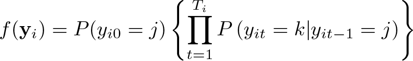
Let N be the total number of agents in the population and K +1 be the total number of states or choice alternatives. Assuming a discrete-time process, y_it represents the state of agent i (i = 1, 2,…, N) at time t (t = 0, 1,…, T_i ). The indicator variable y_it is equal to j (j = 0, 1,…, K) if agent i is in state j at time t. State j = 0 is arbitrarily chosen to indicate entry into or exit from the population. The length of time (T_i ) for which an agent is observed may vary across agents (that is, T_i ≤ T ). Over time period T_i , the row-vector y _i = (y_{i 0} , y_{i 1} ,…, y_iTi) represents the set of transitions of agent i over the K state-space categories. Assuming that the movements of agents follow a first-order Markov process, the probability density function describing the transition process across states can be derived as (Dias and Willekens 2005)

$f\left({\mathbf{y}}_i\right)=P\left(y_i{ }_0=j\right)\left\{{\displaystyle \prod _{t=1}^{T_i}P\left(y_{it}=k|y_{it-1}=j\right)}\right\}$

where P (y_{i 0} = j) is the probability that agent i starts in state j at time t = 0 and P (y_it = k|y_{it −1} = j) is the probability that agent i moves to state k at time t given that it was in state j at time t − 1.

Suppose now that the observed sample of agents is divided into G homogeneous types instead of a single type, where agents of the same type are characterized by a similar Markovian process. The density function of y _i is thus a discrete mixing distribution with G support points (McLachlan and Peel 2000). Assuming heterogeneity, the transition process of agents can be represented by the MMCM formulated as (Vermunt 2010)

$f\left({\mathbf{y}}_i\right)={\displaystyle \sum _{g=1}^{G}P\left(g_i=g\right)P\left(y_i{ }_0=j|g_i=g\right)}\left\{{\displaystyle \prod _{t=1}^{T_i}P\left(y_{it}=k|y_{it-1}=j,g_i=g\right)}\right\}$

Thus, the MMCM has three components. The first term on the right-hand side of (1) represents the probability that agent i belongs to a specific type g. The second and the third terms, respectively, represent the probability that agent i begins in a specific state j and the probability that agent i moves across states during the T_i time period, given that it is of specific type g.

2.1 Specification method

The three components of (1) can be specified as functions of exogenous variables. In this case, the model is fully parametric. Assuming that the states are finite, exhaustive, and mutually exclusive, we use a discrete-choice approach to specify initial states (or entry) and transition probabilities. Furthermore, if independence from irrelevant alternatives can be assumed for the odds ratios, we can use a multinomial specification (Greene 2018). This leads to a multinomial logit expression for the probability of starting in a specific state j and the conditional probability of making a transition from state j to state k. The probability of starting in state j thus writes

$P\left(y_i{ }_0=j|g_i=g,{\mathbf{x}}_{i0}\right)=\frac{\text{exp}\left({\beta }_{j|g}^{\text{'}}{x}_{i0}\right)}{{\displaystyle {\sum }_{k=1}^K\text{exp}\left({\beta }_{k|g}^{\text{'}}{\mathbf{x}}_{i0}\right)}}\left(\forall j,k=1,2,\mathrm{...},K\right)$

2

where β _{j |g} is a vector of parameters specific to each type g and each initial state j and x _{i 0} is the vector of explanatory variables for agent i at time t = 0. One of these vectors is set to zero for identification purposes.

The transition probabilities across states are specified as

$P\left(y_i{ }_t=k|y_{it-1}=j,g_i=g,x_{it-1}\right)=\frac{\text{exp}\left({\theta }_{jk|g}^{\text{'}}{x}_{it-1}\right)}{{\displaystyle {\sum }_{l=1}^K\text{exp}\left({\theta }_{jl|g}^{\text{'}}{x}_{it-1}\right)}}$

3

where θ _{jk |g} is a vector of parameters specific to each type g and each transition jk. Because entries into the population are specified separately from transitions across states, the initial state j in (3) takes the values 1, 2,…, K while the final state k takes the values 0, 1, 2,…, K. Choosing to stay in the same state for two consecutive time periods as the reference scenario sets θ _{jj |g} = 0 ∀g = 1, 2,…, G and ∀j = 1, 2,…, K for identification purposes.

Because agent types are not known beforehand, the probability that an agent belongs to a specific type is also estimated. For this, we use a fractional multinomial logit specification because these probabilities are constrained to be between zero and one (Papke and Wooldridge 1996). Thus, the type-membership probability that agent i belongs to type g is

$P\left(g_i=g|z_i\right)=\frac{\text{exp}\left({\lambda }_g^{\text{'}}{z}_i\right)}{{\displaystyle {\sum }_{h=1}^G\text{exp}\left({\lambda }_h^{\text{'}}{z}_i\right)}}\left(\forall g=1,2,...,G\right)$

4

where λ _g is a vector of parameters and z _i is a matrix of agent characteristics supposed to be constant over time. The vector of parameters λ _G must be normalized to zero for identification.

If a nonparametric form is used for type membership probabilities, the mixing distribution has a nonparametric or discrete-factor interpretation (Pacifico and Yoo 2013). In this case, the mixture model can be viewed as a semiparametric model because we use a nonparametric specification for type membership probabilities and a parametric specification for both the probability of starting in a specific state and the transition probabilities across states. In such a case, the type-membership probability is the same for all agents.

2.2 Expectation-maximization algorithm for the MMCM

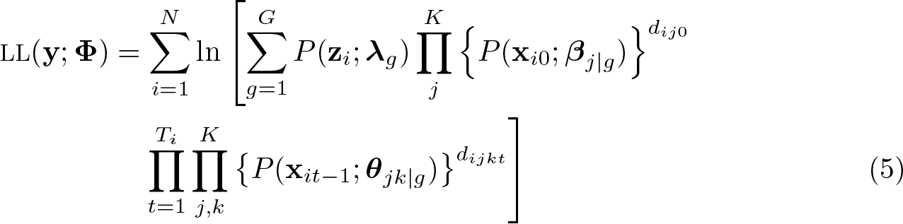
We estimate the parameters of the MMCM using the maximum-likelihood estimation technique. Considering that the observed sample of agents is divided into G homogeneous types, the log-likelihood (LL) function for the parameters of the model is

$\text{LL}\left(y;\Phi \right)={\displaystyle \sum _{i=1}^N\text{In}}\left[{\displaystyle \sum _{g=1}^{G}P\left(z_i;{\lambda }_g\right)}{\displaystyle \prod _j^K{\left\{P\left(x_{io};{\beta }_{j|g}\right)\right\}}^{d_{ij0}}}{\displaystyle \prod _{t=1}^{T_i}{{\displaystyle \prod _{j,k}^K\left\{P\left(x_{it-1};{\theta }_{jk|g}\right)\right\}}}^{d_{ijkt}}}\right]$

5

where Φ = (Φ ₁, Φ ₂ ,…, Φ _G ) is the vector of parameters to be estimated, with Φ _g = ( λ _g, β_{j |g} , θ _{jk |g} ) ∀g = 1, 2,…, G, ∀j = 1, 2,…, K and ∀k = 0, 1, 2,…, K. The indicators d_{ij 0} and d_ijkt , respectively, take the value 1 if agent i starts in state j and moves from state j to state k at time t and zero otherwise.

The expectation-maximization (EM) algorithm developed by Dempster, Laird, and Rubin (1977) simplifies the complex LL function in (5) into a set of easily solvable LL functions by introducing a so-called missing variable. ¹ Let v_ig be a discrete unobserved variable indicating agent type. The random vector v _i = (v_{i 1} , v_{i 2} ,…, v_iG ) is thus g-dimensional with v_ig = 1 if agent i belongs to type g and zero otherwise. Assuming that v_ig is unconditionally multinomially distributed with probability π_g , the complete likelihood for (β, π ), conditional on observing y _c = (y, v), is ²

$\text{LL}\left(y;\Phi \right)={\displaystyle \sum _{i=1}^N{\displaystyle \sum _{g=1}^G{v}_{ig}}}\text{\hspace{0.17em}In\hspace{0.17em}}\left[P\left(z_i;{\lambda }_g\right){\displaystyle \prod _j^K{\left\{P\left(x_{io};{\beta }_{j|g}\right)\right\}}^{d_{ij0}}}{\displaystyle \prod _{t=1}^{T_i}{{\displaystyle \prod _{j,k}^K\left\{P\left({\mathbf{x}}_{it-1};{\mathit{\theta }}_{jk|g}\right)\right\}}}^{d_{ijkt}}}\right]$

6

Because agent type is not observed, the “posterior” probability that agent i belongs to type g (that is, v_ig ) must be derived from the observations. The EM algorithm therefore consists of the following four steps:

Initialization: Arbitrarily choose initial values ${\Phi }^0= ({\Phi }_1^0,{\Phi }_2^0, . . . ,{\Phi }_G^0)$ . To obtain appropriate initial values, we proceed as in Pacifico and Yoo (2013) by randomly assigning each agent to one of the G possible types. Parameters are then estimated for each type.

Expectation: At iteration p + 1 of the algorithm, compute the expected probability that agent i belongs to a specific type g given y _i and parameters Φ ^p . This conditional expected (that is, “posterior”) probability $v_{ig}^{(p+1)}=v_{ig}(y_i;{\Phi }^p)$ is obtained using the following Bayes formula (Dempster, Laird, and Rubin 1977):

$v_{ig}^{\left(p+1\right)}=\frac{P\left(z_i;{\lambda }_g\right){\displaystyle {\prod }_j^K{\left\{P\left(x_{io};{\beta }_{j|g}\right)\right\}}^{d_{ij0}}}{\displaystyle {\prod }_{t=1}^{T_j}{\displaystyle {\prod }_{j,k}^K{\left\{P\left(x_{it-1};{\theta }_{jk|g}\right)\right\}}^{d_{ijkt}}}}}{{\displaystyle {\sum }_{h=1}^{G}P\left(z_i;{\lambda }_h\right){\displaystyle {\prod }_j^K{\left\{P\left(x_{io};{\beta }_{j|h}\right)\right\}}^{d_{ij0}}}{\displaystyle {\prod }_{t=1}^{T_j}{\displaystyle {\prod }_{j,k}^K{\left\{P\left(x_{it-1};{\theta }_{jk|h}\right)\right\}}^{d_{ijkt}}}}}}$

Replacing v_ig in (6) by its expected value $v_{ig}^{(p+1)}$ gives the conditional expectation of the LL function for the complete data.

Maximization: Update Φ ^p by maximizing the complete LL function conditional on the observations. The model parameters are thus updated as

$\begin{array}{l}{\mathbf{\lambda }}^{\left(P+1\right)}=\arg {\max }_{{\mathbf{\lambda }}_g}{\displaystyle \sum _{i=1}^N{\displaystyle \sum _{g=1}^G{v}_{ig}^{\left(p+1\right)}}}\ln \left\{P\left({\mathbf{z}}_i;{\mathbf{\lambda }}_g\right)\right\}\forall g=1,2,\mathrm{....},G-1\\ {\beta }^{\left(P+1\right)}=\arg {\max }_{{\beta }_{j|g}}{\displaystyle \sum _{i=1}^N{\displaystyle \sum _{g=1}^G{v}_{ig}^{\left(p+1\right)}}}{\displaystyle \sum _j^K{d}_{ijo}\ln \left\{P\left({\mathbf{x}}_{io};{\beta }_{j|g}\right)\right\}}\forall j=1,2,\mathrm{....},k-1\\ {\mathit{\theta }}^{\left(P+1\right)}=\arg {\max }_{{\mathit{\theta }}_{jk|g}}{\displaystyle \sum _{i=1}^N{\displaystyle \sum _{g=1}^G{v}_{ig}^{\left(p+1\right)}}}{\displaystyle \sum _{t=1}^{T_I}{\displaystyle \sum _{j,k}^K{d}_{ijkt}\ln }}\left\{P\left({\mathbf{x}}_{it-1};{\mathit{\theta }}_{jk|g}\right)\right\}\hspace{0.17em}\forall j\ne k\end{array}$

The maximization process of the above equations is straightforward. The parameters (Φ ^p ) are updated using v_ig (y _i ; Φ ^p ) as a weighting factor for each observation (Pacifico and Yoo 2013). The built-in mlogit Stata command is used for the estimation of the starting state and the transition probabilities, while the community-contributed command fmlogit (Buis 2008) is used for the type membership probabilities. If a nonparametric form is used for the mixing distribution, the “prior” type membership probability [that is, P (g_i = g)] is the same for all agents and can be derived as

${\pi }_g^{\left(p+1\right)}=\frac{{\displaystyle {\sum }_{i=1}^N{v}_{jg}^{\left(p+1\right)}}}{{\displaystyle {\sum }_{i=1}^N{\displaystyle {\sum }_{h=1}^G{v}_{ih}^{\left(p+1\right)}}}}\hspace{0.17em}\forall g\in G-1$

Iteration: Return to step ii using π ^(p+1) and β ^(p+1), and iterate until the observed LL given by (5) converges, that is, until the relative difference in the LL between two consecutive iterations is sufficiently small. At convergence, the resulting parameters are considered to be the optimal estimators ( $\widehat{\Phi }$ ) given the set of initial values (Φ ⁰) randomly chosen.

2.3 Heuristic strategy

A problem that often occurs in a mixture analysis with several components is that some solutions may be suboptimal. Indeed, the nonconcavity of the LL function in (5) does not make it possible to identify a global maximum in the mixture model, even for mixtures of multinomial logit models (Hess, Bierlaire, and Polak 2007). Given the potential presence of a high number of local maximums, the EM solutions may depend on the initial values chosen for Φ ⁰ (Baudry and Celeux 2015). To increase the chances of obtaining a global maximum in the estimation procedure reported above, we proceed as follows.

First, short-run EMs are used to obtain initial values for long-run EMs. For each short-run EM, the iterative procedure presented in section 2.2 is performed several times with various randomly chosen initial values for the parameters of the model. To do this, the sample is randomly divided into the total number of agent types, and the parameters of the model are estimated separately over each subsample. The resulting parameters are then used in the expectation step of the algorithm to compute the “posterior” probability of agent-type membership. The iterative procedure is stopped after a few iterations, and the resulting parameters that produce the largest LL according to (5) are chosen as the best initial values for long-run EMs.

Second, several long-run EMs are used to obtain the best parameters for the model. For each long-run EM, the iterative procedure is performed until the LL function converges. The parameters that provide the largest LL at the convergence of the EM algorithm are chosen as the global maximum.

3 The mixmcm command

3.1 Syntax

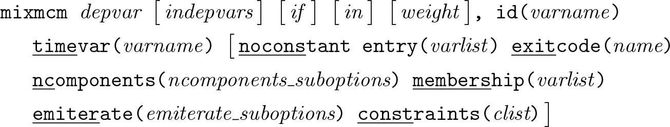
The general syntax for the mixmcm command is

depvar is the dependent variable that indicates agents’ states at each time period. indepvars are optional explanatory variables that enter the specification of transition probabilities. fweights and pweights are allowed; see [U] 11.1.6 weight.

3.2 Options

id( varname ) specifies the variable that identifies agents. mixmcm computes the probability of belonging to a specific homogeneous type for each id(). id() is required.

timevar( varname ) specifies the numeric variable that identifies dates on (or time periods during) which transitions occur. This variable is used to identify the transitions of agents across states. timevar() is required.

noconstant suppresses the constant term (or intercept) in the specification of the transition probabilities. Specifying the noconstant option requires that at least one indepvar be specified.

entry( varlist ) specifies the dependent and independent variables that enter the specification of entry probabilities. Specifying entry()requires that at least the dependent variable indicating the entry state be specified.

exitcode( name ) indicates the modality of depvar that identifies the exit state.

ncomponents([#1 #2 , selcrit( name ) graph( namelist , twoway_options ) save( filename , replace detail) force ]) specifies the number of (unobserved) homogeneous types and related options.

#1 and #2 indicate the range for the number of components. If both #1 and #2 are specified, mixmcm will fit the #1 − #2 MMCM, starting from the model with the #1 component or components and proceeding to the model with the #2 components to identify the optimal number of components within this range based on the selection criterion specified in the suboption selcrit()(see below). Unless the suboption force is specified (see below), the estimation will stop automatically when the optimal number of components is found, and the results will solely be displayed for this optimal number of components. If only #1 is specified, mixmcm will estimate only the parameters for this number of component or components, and the corresponding results will be displayed. A standard (homogeneous) MCM will be fit if the specified number of components is #1 = 1. By default, a two-components MMCM is fit.

selcrit( name )specifies the information criterion used to select the optimal number of components within the #1 to #2 range. The available information criteria are aic, bic, aic3, or caic (the default). See Andrews and Currim (2003) for a discussion on information criteria for the retention of the optimal number of components.

graph( namelist , twoway_options ) specifies that a graph for the information criteria specified in namelist be drawn for the number of components in the #1 to #2 range. The graph() suboption thus requires that at least one information criterion among aic, bic, aic3, or caic be specified in namelist. Users can manage the graph using standard twoway_options.

save( filename , replace detail) saves the information criteria for the numbers of components estimated within the #1 to #2 range in filename. Specifying replace as a suboption will overwrite an existing filename. If detail is specified as a save() suboption, the resulting parameters for all the estimated numbers of components will be jointly saved.

force indicates that models should be fit for all the numbers of components within the #1 to #2 range, even when the optimal number of components is found to be smaller than #2 based on selcrit(). Therefore, estimations will continue until #2 in either case.

membership( varlist ) specifies the independent variables to be included in the specification of the component-membership probabilities. These variables must be constant over time for each agent. The parametric form for the mixing distribution is fmlogit, which allows the dependent variable to lie between 0 and 1. Specifying membership() requires that at least one explanatory variable be specified. By default, type-membership probabilities will be estimated nonparametrically (see Train [2008]).

emiterate ([ lr( #1 #2 , eps ) sr( #1 #2 ) seed( # ) emlog) ]) specifies suboptions for the EM algorithm.

lr( #1 #2 , eps ) specifies the number of long-run EMs (#1) to be performed, the maximum number of iterations (#2) to be used for each long-run EM, and the convergence criterion to stop the iterations (eps), respectively. The default is lr(5 100, 0.0000001). eps is the tolerance used in the log-likelihood maximization: mixmcm declares convergence when the proportional increase in the log likelihood over two consecutive iterations is less than the specified eps.

sr( #1 #2 ) specifies the number of short-run EMs (#1) and the maximum number of iterations (#2) for each short-run EM. The default is sr(5 5).

seed( # ) sets the pseudouniform random-numbers seed. Initial parameters for the EM estimation are randomly chosen using the same seed. The default is seed(123456). The seed is a local macro that replaces seeds that have been chosen by users outside of the command.

emlog displays the logs for long-run EM iterations.

constraints( clist ) lists the constraints to impose on transition probabilities. Each constraint listed in clist must be specified as constraint # p_initialstate_finalstate = 0, where # is the number that identifies the constraint. For now, transition probabilities can be constrained only to be 0, and this constraint applies across all components.

4 Examples

To illustrate how mixmcm works, the command is used to estimate size-transition probabilities in the French farming sector under the assumption of a heterogeneous farm population. Data are provided by the R´eseau d’Information Comptable Agricole (RICA), the French implementation of the Farm Accountancy Data Network. ³ RICA collects technical and economic information on a sample of commercial French farms on an annual basis. The data are freely available online from the RICA France website (see http://agreste.agriculture.gouv.fr/enquetes/reseau-d-information-comptable/).

For this illustration, we use data from 2000 to 2010. The 11 (annual) databases were appended together, leading to an unbalanced panel where idnum is the unique farm identifier and year is a generated time variable that will be used as timevar() in mixmcm. Some modifications of the full original database were necessary to be able to use it with mixmcm. First, the population was broken down into three size categories (K = 3) according to the economic size variable pbuce, which measures the production potential of farms in terms of Euros of standard output (SO). The resulting category variable, which will be used as depvar in mixmcm, therefore consists of three categories, namely, medium farms (denoted mediumwith pbuce < 100,000 Euros of SO), large farms (denoted large with 100,000 ≤ pbuce < 250,000 Euros of SO), and very large farms (denoted vlarge with pbuce ≥ 250,000 Euros of SO). We then restricted the sample to farms that have existed in the database for at least two consecutive years to observe at least one transition. We also retained only a subset of variables and renamed them for use in our examples. The new database, mixmcm.dta, is organized as follows:

The variables surplus, istock, icap, and debtr are the gross operating surplus, initial stock in Euros, initial capital in Euros, and the debt ratio of the farm in percent, respectively. The other (indicator) variables (crop = 1 if the farm specializes in field crop production, corp = 1 if the farm has corporate legal status, educ = 1 if the farmer has a higher-level education, and young = 1 if the farmer is under 41) were derived from original variables for our specific examples. ⁴

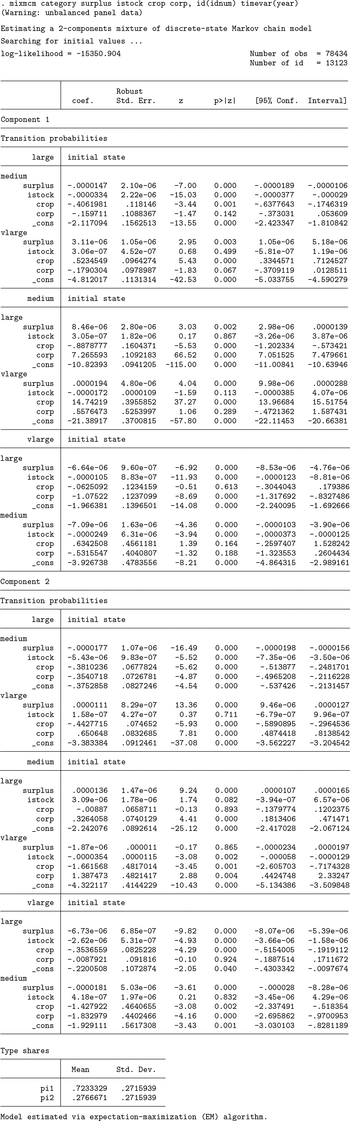
4.1 Fitting a simple two-component MMCM

To illustrate the basic use of mixmcm, we first fit a two-component MMCM without considering entries or exits. In this example, we specify transition probabilities as a function of four explanatory variables, namely, surplus, istock, crop, and corp. The parameters of the mixing distribution are estimated nonparametrically. As mentioned in section 2.1, the resulting model is therefore considered to be semiparametric.

The table above reports the resulting coefficients of the explanatory variables for each component (that is, the degree to which they contribute to explaining the odds ratios, where remaining in the initial state is the reference scenario). As such, the values of the coefficients are not directly interpretable (see section 5 for the derivation of elasticities). If one focuses on the signs, however, it is evident that the contributions of the coefficients differ across components. For example, the variable corp has a negative (−0.179) effect on the odds ratio {P (large → vlarge)}/{P (large → large)} for the first component, while this impact is positive (0.651) for the second component. The parameters pi1 and pi2, respectively, are the resulting shares of type 1 and type 2 in the studied sample.

The standard errors reported in the table are obtained from the official Stata command mlogit, using the option vce(robust) in the model specification. The variance– covariance matrix is thus obtained by the Huber/White/sandwich estimator. Indeed, mixmcm performs multiple weighted multinomial logit estimations according to the number of types × number of initial states specified. Each weighted multinomial logit is estimated separately. For each estimation, we use the robust or sandwich estimator of the variance–covariance matrix, assuming that explanatory variables (X _it ) and the error terms (ǫ_it ) are uncorrelated. With these assumptions and a few technical regularity conditions, each weighted mlogit yields consistent parameter estimates and standard errors. ⁵ We can thus use the resulting mixmcm parameter estimates and standard errors for valid statistical inference about the coefficients (see section 5).

4.2 Specifying entry, exit, type membership, and constraints on transition probabilities

In this second example, we fit a two-component MMCM that includes entry and exit. We also specify a set of explanatory variables for entry and type membership probabilities and impose constraints on some transition probabilities.

We now consider farms that leave the sample before the final year of the panel (2010) as exits. We thus add a new category, exits, to the variable category.

Similarly, we now consider farms that enter the sample after the first year of the panel (2000) as entries. We thus generate a new variable, entry_class, that indicates the category in which farms are observed for the first time in the sample.

We also generate new variables to be used in the specification of the type-membership probabilities. To ensure that these probabilities do not vary over time, we take the mean of the continuous variable debtr and the mode of the dummy variables educ and young.

Finally, we specify two constraints on the transition probabilities: the probability of moving from the medium category to the vlarge category is set to zero and vice versa.

The MMCM under the above specification is therefore fit as

Compared with the first example, this one has three additional sets of parameters. First, the parameters for the exit state now appear in the table of results. Because entries are estimated separately, the total number of initial states remains the same as in example 1.

Second, the parameters for the probability of entering in a given size category are reported in the section Entry probabilities of the table of results. The coefficients represent the contribution of the explanatory variables in explaining the odds ratios, with the large category as the reference. ⁶ The parameters for the odds ratio {P (medium)}/{P (large)} in component 1 are set to zero, meaning that there are not enough observations for the identification of these parameters in this component. As in example 1, the effect of the explanatory variables also differs across components. For example, the results show that the variable corp has a larger positive effect on the odds ratio {P (vlarge)}/{P (large)} for farms that belong to the first component. The estimated coefficient is 4.197 for farms belonging to component 1 and only 0.578 for farms belonging to component 2.

Third, the parameters for the membership probabilities are given in the Membership probabilities section of the results table, after the resulting type shares pi1 and pi2. The coefficients represent the contribution of the explanatory variables in explaining the odds ratios using the probability of belonging to component 1 as the reference. All three chosen variables (meandebtr, modeeduc, and modeyoung) have a positive effect on the probability of belonging to component 2 versus component 1.

Finally, one can verify that the parameters for the transition probabilities that were constrained to zero are not estimated by the model, because they appear as set to zero and indicated as (omitted) in the table of results.

4.3 Choosing the optimal number of components

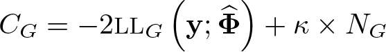
In this last example, we illustrate how the number of components can be chosen by relying on statistical information rather than a priori knowledge on the total number of components as in the previous examples. In this case, the criteria used to select the most relevant model are generally based on the value of $-2L{L}_G(y;\widehat{\Phi })$ of the model, where $L{L}_G(y;\widehat{\Phi })$ represents the maximum LL estimate adjusted for the number of free parameters in the model. The basic principle here is parsimony: all other things being equal, the model with fewer parameters should be preferred. In the case of latent class models such as the MMCM, the selection of the total number of types G is generally based on the following criterion (Andrews and Currim 2003; Dias and Willekens 2005)

$C_G=-2L{L}_G(y;\widehat{\Phi })+K\times N_G$

where N_G is the total number of free parameters of a model with G types. Different values for the penalizing factor κ lead to the various well known information criteria: the Akaike information criterion (AIC) with κ = 2 and the Bayesian information criterion (BIC) with κ = log(n) (Andrews and Currim 2003). Other information criteria can also be derived such as the consistent Akaike information criterion (CAIC) with κ = log(n) + 1 and a modified AIC (AIC3) with κ = 3 (Andrews and Currim 2003). For each of these heuristic criteria, smaller values indicate more parsimonious models.

As an illustration, we search for the optimal model for our RICA data by letting the number of unobserved types vary within the range of one to five components. We also set alternative numbers of short-run and long-run EM iterations to increase the chances of obtaining a global maximum in each case. We choose the optimal number of components based on the CAIC criterion (the default), but a graph is drawn for all available information criteria. Finally, we also save the estimated parameters for all models in a file that can be used for further analysis. To do so, we use mixmcm as follows:

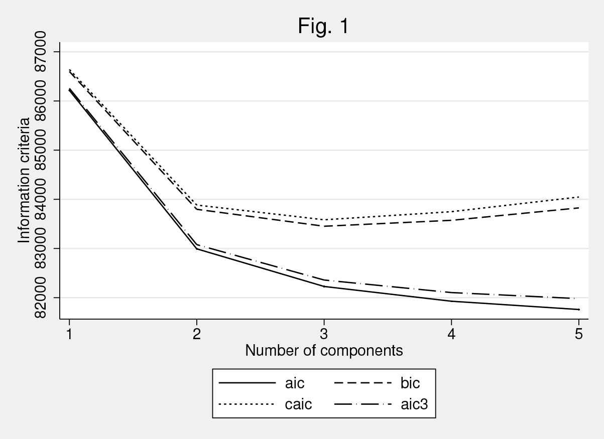
Figure 1 shows that, based on the model specification and according to the CAIC, a mixture of three types of farms should be chosen as the optimal number of components. It also shows that the BIC is consistent with the CAIC in identifying three components while, according to the AIC and AIC3, a higher number of farm types should be preferred.

Figure 1.

Comparison of statistical information criteria for different numbers of unobserved farm types

In these two latter cases, however, the improvement in the values of the criteria is relatively small when specifying more than three types so that three components may overall be a relevant compromise.

The command output displays the results regarding the optimal number of components. The corresponding table is not reported here because it is essentially similar to that of example 2, the difference being that it reports the results for three components instead of two. Additionally, because we use the suboption force for the ncomponents() option, the information criteria and the full set of estimated parameters for all fitted models (from one to five components) are saved to disk in the specified filename icbtable; an excerpt of this file is provided in the appendix. Finally, mixmcm stores the following in e():

The estimated coefficients and the variance–covariance matrices for the transition probabilities and for component membership are given in matrices e(b_tpm), e(V_tpm), e(b_proba), and e(V_proba), respectively. The matrices e(pi) and e(Cns_tpm) contain the components’ shares and the constraints on transition probabilities, respectively. Standard deviations are also reported for the shares of each type component in the matrix e(pi). The elements of matrix e(Cns_tpm) take the value 1 if the respective transition probability is constrained to be 0. Otherwise, the elements of the matrix are set to 0.

5 Hypothesis testing, transition probability, and elasticity derivation

Because the parameters estimated by the mixmcm command usually are not directly interpretable in applied work, this section demonstrates how to derive empirically useful information from these estimated parameters. For example, they can be used to conduct hypothesis testing to compare specific parameters across components. They can also be used to compute transition probabilities and derive probability elasticities and structure elasticities.

To perform postestimation calculations for hypothesis testing, transition probability computation, and elasticity derivation, we must first put the vector of coefficients and the variance–covariance matrix in b and V, respectively. To do this, we can use the following subroutine:

Then, the above subroutine must first be called just before using any Stata postestimation command for the calculations. In the following, we present how to perform hypothesis testing, transition probability, and elasticity derivation for example 1 but the method would apply to any MMCM model fit with the mixmcm command.

5.1 Hypothesis testing

Wald tests of simple and composite linear hypotheses about the parameters of the model can be performed to conduct hypothesis testing. For example, users can test whether the estimated parameters are different from zero as follows:

i) A test on a specific parameter of a specific transition for a specific component.

ii) A joint test on all the parameters of a specific transition and a specific component.

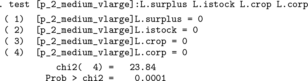
iii) A joint test on all the parameters of all the transitions for all components.

For the last example, we report only the first five lines of the output to save space. The Wald test is performed for all the estimated parameters of all the transitions, including the base outcome identified with the prefix o for each explanatory variable.

In any of the specific examples above, considered Wald tests show that the tested parameters all are different from 0 at the 1% significance level at least. ⁷

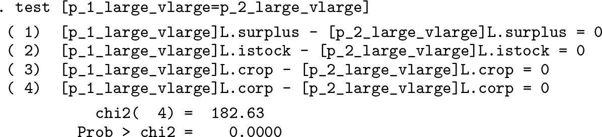
Users may also test whether the same parameters for two different components are different from each other, that is, whether the MMCM identify agent types characterized by specific parameter values.

i) A test on specific parameters for specific transition probabilities across two specific components.

ii) A joint test on all the parameters for a specific transition across two specific components.

In these specific examples, the considered Wald test shows that the two components, that is, the two endogenous types of farms, are characterized by different estimated parameter values at the 0.1% significance level at least for the probability to move from category large to the category vlarge. Of course, such tests can be performed for any transition and whatever the number of components.

5.2 Transition probabilities

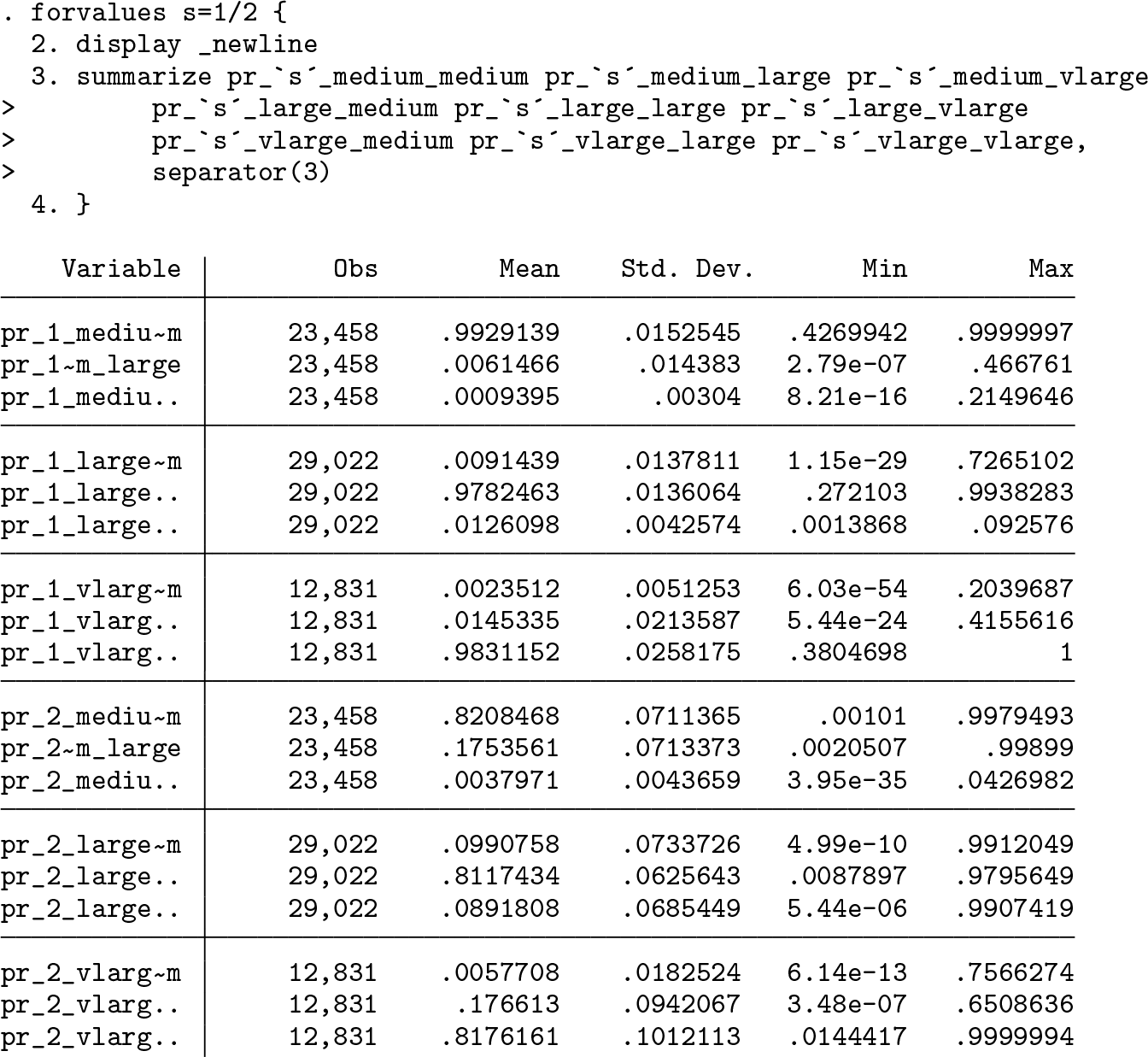
As mixmcm performs multiple multinomial logistic regressions to estimate the parameters, the predict Stata command cannot be used to directly derive transition probabilities. ⁸ Considering the results from example 1, we can compute transition probabilities using (3). To save space, we report the code lines for the calculations in the appendix. The transition probabilities are reported below.

The results in the table above show that transition probabilities differ across the two considered components. The farms in type 1 exhibit a very high probability to remain in the same category of size two consecutive years (above 0.95), whatever their initial category. These probabilities are lower for farms in type 2 (below 0.85), which means that those farms are more likely to move across the size categories over the years.

The above procedure can be applied to compute entry probability from (2) and probability of type membership from (4) if a parametric form is used for the mixing distribution. ⁹

5.3 Probability elasticities

As mentioned earlier (see section 4.1), the impacts of explanatory variables on logodds ratios are difficult to interpret directly (Greene 2018). In this case, the impacts of explanatory variables are rather given with respect to transition probabilities, as measured in terms of elasticities. “Probability elasticities” thus measure the (relative) effect of a 1% change in the ith explanatory variable on the transition probabilities (Zepeda 1995). In our mixture model, average transition-probability elasticities from one period to the next for farms belonging to a specific type g can be derived as

${\mathit{\delta }}_{jk|g}=\left({\beta }_{jk|g}-{\displaystyle \sum _{l=1}^K{\beta }_{jk|g}{p}_{jl|g}}\right)\overline{\mathbf{x}},\forall j,k\in k,\forall g\in G$

where δ _{jk |g} is a vector gathering elasticities at the means over the period T − 1 of the explanatory variables in vector x on the transition probability from category j to category k conditional on belonging to type g (p_{jk |g} ); and β _{jk |g} is the corresponding vector of estimated parameters. ¹⁰

Considering again example 1, we can use the transition probabilities computed in section 5.2 to derive transition-probability elasticities using the nlcom Stata command as follows:

The resulting coefficients in the table above show that, for example, a 1% increase in the amount of farm total surplus will decrease the probability to remain in the medium category of size two consecutive years by about 0.005% for farms in type 1 but by about 0.164% for those in type 2.

The above procedure can be applied to derive entry-probability elasticities and probability elasticities for type membership if a parametric form is used for the mixing distribution.

5.4 Structure elasticities

The estimated parameters can be also used to derive “structure elasticities”. In the context of our agricultural examples, structure elasticities measure the impacts of the exogenous variable on the distribution of farms across size categories. In other words, farm structure elasticities measure the variation in percentage of the total number of farms in a specific category k for a 1% change in the ith explanatory variable. In our mixture model, average structure elasticities from one period to the next can be derived as follows.

The total number of farms in a specific category k at any specific time can be obtained as

$n_k={\displaystyle \sum _{j=1}^G{\pi }_g}{\displaystyle \sum _j^K{n}_j\times p_{jk|g\text{'}}}\forall k\in k$

where π_g is the probability of belonging to type g, n_j is the total number of farms in category j at the preceding time period, and p_{jk |g} is the probability of making a transition from category j to category k from one year to the next. The vector of farm structure elasticities is then defined as

${\eta }_k=\frac{\partial n_k}{\partial \mathbf{x}}\times \frac{\overline{\mathbf{x}}}{n_k}$

where $\overline{x}$ is the vector of means of the explanatory variables over the period T − 1.

In (7), only transition probabilities depend on exogenous variables. Farm structure elasticities can therefore be obtained using the corresponding transition-probability marginal effects. Average structure elasticities from one period to the next are thus given by

${\mathit{\eta }}_k=\left({\displaystyle \sum _{g=1}^G{\pi }_g}{\displaystyle \sum _{j=1}^K{n}_j}\times \frac{\partial p_{jk|g}}{\partial \mathbf{x}}\right)\frac{\overline{\mathbf{x}}}{n_k}$

where (∂p_{jk |g} )/(∂ x) are the marginal effects at the means of the corresponding explanatory variables. ¹¹

Considering example 1, we can derive structure elasticities at the means of explanatory variables by following three steps: i) computing farm numbers across size categories from the sample; ii) computing predictive margins at the means of the explanatory variables using the estimates; iii) deriving structure elasticities using the distribution of farms across size categories and predictive margins.

The coefficients in the table above show that the number of farms in the medium size category will decrease by 0.171% if farm total surplus increases by 1% from one year to the next. Because in example 1 we do not consider exits or entries, these 0.171% of medium farms will move to the large category for 0.016% and to the vlarge category for 0.155%.

Structure elasticities can also be derived, accounting for entries and exits as in example 2. To do this, we can use the same procedure considering the corresponding predictive margins.

6 Discussion

The community-contributed mixmcm command proposed here enables the estimation of MMCMs in Stata. The command is especially adapted to fit mixtures of nonstationary MCMs, accounting for entries and exits in the population under study. The examples presented in the preceding sections can easily be reproduced using other data provided that they are organized or rearranged in a similar fashion.

Future developments of the command will take three directions. First, the specification of constraints will be made more general to allow for constraining transition probabilities for only a subset of components. This would, for instance, allow for the implementation of the so-called mover–stayer model, a restricted form of the MMCM that has been widely applied in the literature (Saint-Cyr 2017). In this model, only two types of agents are considered, the “movers”, who follow a standard Markovian process, and the “stayers”, who always remain in their starting category. In this setting, the stayers’ transition matrix degenerates to a diagonal matrix, where all but the diagonal transition probabilities are constrained to zero while the diagonal probabilities are constrained to unity, and the movers’ transition matrix may be unconstrained. Generalizing the constraints syntax in mixmcm would thus allow for the implementation of such a model, or even a more sophisticated model composed of one stayer type and several mover types. Second, the command will also be improved to be able to account for other parametric forms (logit, Poisson, etc.) of the mixing distribution, for which there is already some precedent in the literature (Lindsay and Lesperance 1995; Greene and Hensher 2003; Train 2009). Finally, specific postestimation commands will be incorporated so that deriving second-order parameters of interest such as those exemplified in section 5 will be directly and easily available with no further coding as stand-alone in-line commands.

Supplemental Material

Supplemental Material, st0556 - mixmcm: A community-contributed command for fitting mixtures of Markov chain models using maximum likelihood and the EM algorithm

Supplemental Material, st0556 for mixmcm: A community-contributed command for fitting mixtures of Markov chain models using maximum likelihood and the EM algorithm by Legrand D. F. Saint-Cyr and Laurent Piet in The Stata Journal