lsemantica: A command for text similarity based on latent semantic analysis

Abstract

In this article, I present the lsemantica command, which implements latent semantic analysis in Stata. Latent semantic analysis is a machine learning algorithm for word and text similarity comparison and uses truncated singular value decomposition to derive the hidden semantic relationships between words and texts. lsemantica provides a simple command for latent semantic analysis as well as complementary commands for text similarity comparison.

1 Introduction

The semantic similarity of two text documents is a highly useful measure. Knowing that two documents have a similar content or meaning can, for example, help to identify documents by the same author, measure the spread of information, or detect plagiarism. There are two main problems when attempting to identify documents with similar meaning. First, the same word can have different meanings in different context. Second, different words can have the same meaning in other contexts. Thus, using just the words counts in documents as a measure of similarity is unreliable. The alternative of reading and hand-coding documents already becomes prohibitive for a few hundred documents.

By providing a reliable measure of semantic similarity for words and texts, latent semantic analysis (LSA) provides a solution to this problem. LSA was developed by Deerwester et al. (1990) for the task of automated information retrieval in search queries. In search queries, it is important to understand the relationships and meanings of words because just using the query terms often leads to unsatisfying search results. LSA improves results by accounting for the relationships and potential multiple meanings of words. It is this property that makes LSA applicable for a variety of different tasks, including the following:

Similarity of words (Landauer, Foltz, and Laham 1998)

Similarity of texts (Gomaa and Fahmy 2013; Iaria, Schwarz, and Waldinger 2018)

Computer-guided summary writing (Wolfe et al. 1998; Franzke et al. 2005)

Automated essay grading (Kintsch 2002; Miller 2003)

Assessing discourse coherence (Foltz 2007)

For all of these applications, LSA derives the hidden semantic connection between words and documents by using truncated singular value decomposition, the same transformation used in principal component analysis. Principal component analysis uses truncated singular value decomposition to derive the components that explain the largest amount of variation in the data. Similarly, truncated singular value decomposition enables LSA to “learn” the relationships between words by decomposing the “semantic space”. This process allows LSA to accurately judge the meaning of texts. While LSA uses word cooccurrences, LSA can infer much deeper relations between words.

Landauer (2007) compares the workings of LSA with a problem of simultaneous equations. For two equations A+2B = 8 and A+B = 5, neither equation alone is enough to infer the values of A or B. When one combines the two equations together, it becomes straightforward to calculate the respective values for A and B. Similarly, the meaning of a document is based on the sum of the meaning of its words: meaning_document = Σ(meaning_word1 ,…, meaning_wordn). For a computer, it is not possible to infer the meaning of the words based on one document alone, but LSA can “learn” the meaning of words using the large set of simultaneous equations provided by all documents in the corpus.

To illustrate the capabilities of LSA, Landauer (2007) provides the following example. On the one hand, the phrases “A circle’s diameter” and “radius of spheres” are judged by LSA to have similar meaning, despite having no word in common; on the other hand, the phrase “music of the spheres” is judged as dissimilar by LSA, despite using similar words. Thus, text similarity comparison using LSA is preferable to just using the raw word counts in each document because word frequencies completely ignore multiple meanings of words. Furthermore, LSA also outperforms more recent machine learning algorithms when it comes to document similarity comparison (Stevens et al. 2012).

In this article, I introduce the lsemantica command, which provides a solution for using LSA in Stata. lsemantica further facilitates the text-similarity comparison in Stata with the lsemantica_cosine command. In this way, lsemantica further improves the text analysis capabilities of Stata. Stata already allows one to calculate the Levenshtein edit distance with the strdist command (Barker and Pöge 2012), and the txttool command (Williams and Williams 2014) facilitates the cleaning and tokenizing of text data. Moreover, Schwarz’s (2018) ldagibbs command allows one to run latent Dirichlet allocation in Stata. While ldagibbs can group documents together by similar topics, lsemantica is preferable in cases where one is predominately interested in how similar documents are.

2 Decomposing the semantic space using LSA

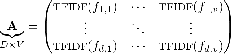
This section describes how truncated singular value decompositions allows LSA to retrieve connections between words. First, lsemantica creates a so-called bag-of-words representation of the texts in the string variable. In this process, lsemantica creates a document-term matrix A. This matrix contains a row for each document d ∈ D and a column for each unique term, that is, words, in the vocabulary V. Each cell in A contains f_d,v , the number of times term v appears in document d:

$\underset{D\times v}{\underbrace{\text{A}}}=\left(\begin{array}{ccc}{f}_{1,1}& \dots & f_{1,v}\\ ⋮& \ddots & ⋮\\ f_{d,1}& \cdots & f_{d,v}\end{array}\right)$

Second, lsemantica reweighs the word frequencies f_d,v in the matrix A by their termfrequency-inverse-document-frequency (TFIDF). Here f_d,v is replaced by TFIDF(f_d,v ) = {1+log(f_d,v )}×[log{(1+D)/(1+d_v )}+1], where d_v is the number of documents in which term v appears. The TFIDF reweighting reduces the weights of words that appear in many documents because these words are usually less important for the overall meaning of documents. After the TFIDF reweighting, the matrix A contains

$\underset{D\times v}{\underbrace{\text{A}}}=\left(\begin{array}{ccc}\text{TFIDF}{f}_{1,1}& \dots & \text{TFIDF}{f}_{1,v}\\ ⋮& \ddots & ⋮\\ \text{TFIDF}{f}_{d,1}& \cdots & \text{TFIDF}{f}_{d,v}\end{array}\right)$

Finally, lsemantica applies singular value decomposition to the reweighted matrix A. This process is represented in figure 1. Singular value decomposition transforms A, of rank R, into three matrices such that A = UΣW ^T , where U is a D × R orthogonal matrix, W ^T is a R × V orthogonal matrix, and Σ is a R × R diagonal matrix (black boxes in figure 1). Afterward, lsemantica truncates the resulting matrices by removing the rows and columns associated with the smallest eigenvalues in the matrix Σ until only the user-chosen number of eigenvalues C remains. This truncation thereby reduces the dimensions of the matrices to C components such that U becomes U _C of dimension D × C, Σ becomes Σ _C of dimension C × C, and W ^T becomes $W_C^T$ of dimension C × V (shaded areas in figure 1).

Figure 1.

LSA graphical representation ¹

The number of components C that should be preserved during truncation is usually chosen based on the size of the vocabulary. Martin and Berry (2007) suggest that 100 ≤ C ≤ 1000 usually leads to good results. During truncation, the entries of the original matrix A change as the number of components is reduced. In the end, this process results in the best rank-C approximation of the original matrix A, called A _C . The truncation process is of utmost importance because it reduces the components of the semantic space to the C most important ones.

The output of lsemantica is then based on U _C × Σ _C , a D × C document-component matrix that can be used to compare the similarity of documents. The individual components of the document-component matrix represent the reduced dimensions of the semantic space. These components capture the semantic relationships between the individual documents. Moreover, lsemantica can save the matrix ${\mathbf{W}}_C^T$ , which allows one to compare the similarity of words. As illustrated by the example in the introduction, even documents that contain completely different words can be judged to be similar by LSA if the words appear together in similar semantic contexts.

3 Stata implementation

This section describes how the lsematica command allows running LSA in Stata. With lsematica, each document the user wants to use for LSA should be one observation in the dataset. If documents consist of thousands of words, users can split the documents into smaller parts, for example, paragraphs, to process each part separately. In any case, only one variable should be used for the text strings. ² Furthermore, nonalphanumerical characters should be removed from the strings.

The lsemantica command is started by specifying the variable that contains the text. There is an option to choose the number of components for truncated singular value decomposition. The options of lsemantica also allow one to remove stop words and short words from the text string. The txttool command (Williams and Williams 2014) provides more advanced text-cleaning options, if required. lsemantica also provides two options to reduce the size of the vocabulary. These options are helpful in cases where truncated singular value decomposition requires a long time because of the size of the vocabulary.

3.1 Syntax

lsemantica varname [, components( integer ) tfidf min_char( integer ) stopwords(_string ) min_freq( integer ) max_freq( real ) name_new_var( string ) mat_save path( string )]

3.2 Options

components( integer ) specifies the number of components the semantic space should be reduced to by lsemantica. The number of components is usually chosen based on the size of the vocabulary. The default is components(300).

tfidf specifies whether TFIDF reweighting should be used before applying the truncated singular value decomposition. In most cases, TFIDF reweighting will improve the results.

min_char( integer ) allows the removal of short words from the texts. Words with fewer characters than min_char( integer ) will be excluded from LSA. The default is min_char(0).

stopwords( string ) specifies a list of words to exclude from lsemantica. Usually, highly frequent words such as “I”, “you”, etc., are removed from the text because these words contribute little to the meaning of documents. Predefined stop word lists for different languages are available online.

min_freq( integer ) allows the removal of words that appear in fewer documents. Words that appear in fewer documents than min_freq( integer ) will be excluded from LSA. The default is min_freq(0).

max_freq( real ) allows the removal of words that appear frequently in documents. Words that appear in a share of more than max_freq( real ) documents will be excluded from LSA. The default is max_freq(1).

name_new_var( string ) specifies the name of the output variable created by lsemantica. These variables contain the components for each document. The user should ensure that name_new_var( string ) is unique in the dataset. By default, the name of the variable is component_, so the names of the new variables will be component_1–component_C, where C is the number of components.

mat_save specifies whether the word-component matrix should be saved. This matrix describes semantic relationships between words. By default, the matrix will not be saved.

path( string ) sets the path where the word-component matrix is saved.

3.3 Output

lsemantica generates C new variables, which are the components generated by the truncated singular value decomposition. As described in the previous sections, these components capture the semantic relationships of documents and allow one to calculate the similarity between documents.

The similarity of documents based on LSA is usually measured by the cosine similarity of the component vectors of each document. The cosine similarity of two documents d1 and d2 and their respective document-component vectors δ _{d 1} and δ _{d 2} is defined as

$\text{cosine\_sim(}{d}_1\text{,}{d}_{\text{2}}\text{)}=\frac{{\displaystyle \sum { }_{c=1}^C\left({\delta }_{d1,c}\times {\delta }_{d2,c}\right)}}{\sqrt{{\displaystyle \sum { }_{c=1}^C}}{\delta }_{d1,c}\times \sqrt{{\displaystyle \sum { }_{c=1}^C}}{\delta }_{d2,c}}$

The cosine similarity is hence the uncentered version of the correlation coefficient. The cosine similarity is 1 for highly similar documents and −1 for completely dissimilar documents. When one uses LSA, the cosine similarity usually lies within the unit interval. Only for highly dissimilar documents will the cosine similarity be negative.

lsemantica further provides the lsemantica_cosine command to facilitate the analysis of the cosine similarity. lsemantica_cosine calculates the cosine similarity for all documents and stores it in Mata. ³ Furthermore, lsemantica_cosine can provide summary statistics for the cosine similarity and find highly similar documents. A separate help file explains the syntax of lsemantica_cosine.

4 Example

The example dataset contains the title of 41,349 articles published in economic journals from 1980 to 2016. After one loads the data, nonalphanumerical characters are removed from the title strings in preparation for LSA.

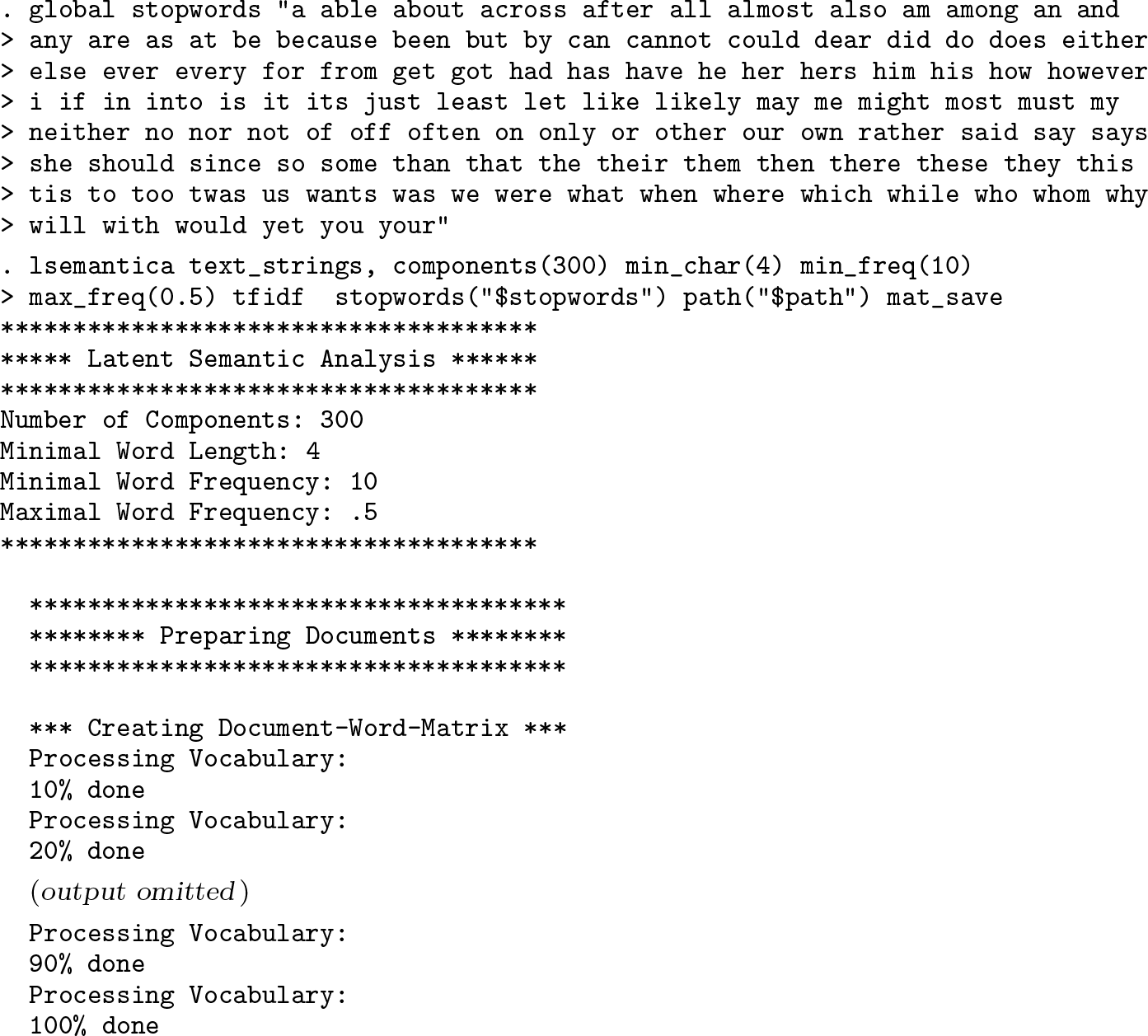
LSA is then started by simply calling the lsemantica command. First, lsemantica prepares the documents and produces the document-term matrix. lsemantica also removes words shorter than 4 characters and words that appear in fewer than 10 documents or in more than half of all documents from the data. Furthermore, stop words are removed from the data. The resulting document-term matrix is then reweighed using TFIDF. The command reports every time when 10% of the vocabulary has been processed.

If documents do not have any words left after the text cleaning, lsemantica will remove these observations from the data because they interfere with the truncated singular value decomposition. lsemantica reports which documents have been removed from the data as well as the size of the vocabulary. In the example, 167 documents are removed. The removal of documents is mainly due to the option min_freq(10). The dataset, for example, contains an article simply titled “Notches”. Because the word “Notches” appears only in the title of three articles, it is not included in the vocabulary.

Next, lsemantica calculates the truncated singular value decomposition, which is computationally intensive and can take some time. In some cases, Stata becomes unresponsive during this process. The time required for the truncated singular value decomposition increases with the size of the document-term matrix and hence with the number of documents and the size of the vocabulary. ⁴

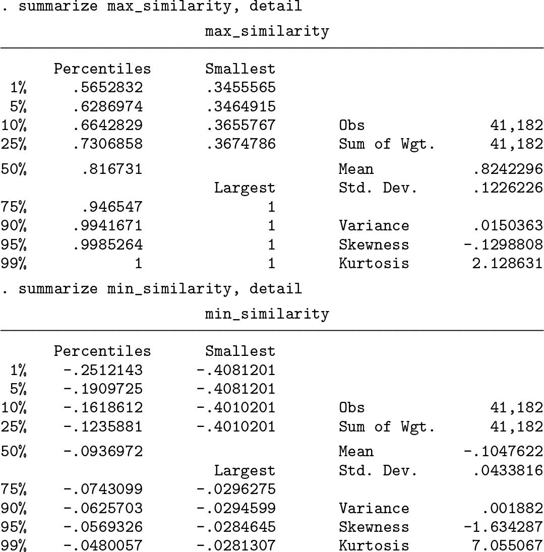
After lsemantica is finished running, one can begin to analyze the similarity of documents by calculating the cosine similarity between the component vectors using the lsemantica_cosine command. ⁵ The resulting cosine similarity matrix is stored in Mata because of its dimensions. If required, the full cosine similarity matrix can be retrieved from Mata using getmata (cosin_*) = cosine_sim after the lsemantica_cosine command. lsemantica_cosine also allows one to calculate the average similarity as well as the maximal and minimal similarity to other article titles.

Furthermore, lsemantica_cosine can find the most similar articles for each of the articles in the data. In the example, the 10 most similar articles are calculated. Afterward, the five most similar article titles for the first article in the data are listed. One can see that LSA accurately identified highly similar articles all discussing questions of labor supply.

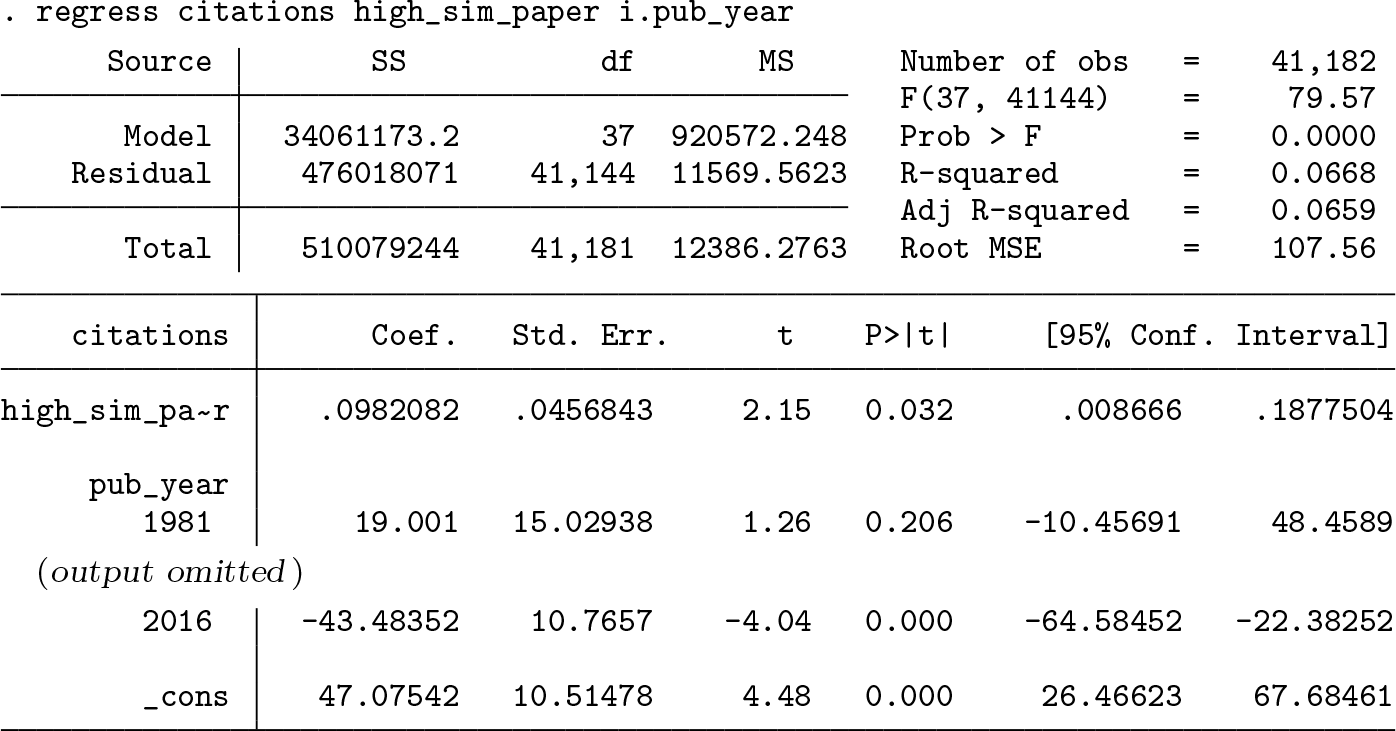
lsemantica can calculate the number of articles to which the original article is highly similar. In the example, a cutoff for the cosine similarity of 0.75 was chosen. The Mata code generates a new variable called high_sim_articles containing the number of articles published afterward that have a cosine similarity above this cutoff. The example data also contain the number of citations for each article. Hence, one can estimate a regression of the number of similar articles on the number of citations. The regression reveals a significant positive relationship between the two variables.

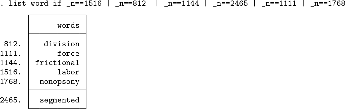
Finally, lsemantica can compare semantic relationships and the similarity of words. Using lsemantica_word_comp, one can import the word-component matrix stored by lsemantica. Again, lsemantica_cosine can be used to calculate the cosine between the words in the data and find the most similar words. The example shows that lsemantica identifies that the words “labor”, “force”, “segmented”, “division”, “frictional”, and “monopsony” are related to one another.

5 Conclusion

LSA has been proven to be a versatile text analysis algorithm. lsemantica brings LSA to Stata and can help researchers to more accurately measure the similarity of text documents with the lsemantica_cosine command. Thereby, lsemantica opens up new ways to analyze text data in Stata.

Supplemental Material

Supplemental Material, st0552 - lsemantica: A command for text similarity based on latent semantic analysis

Supplemental Material, st0552 for lsemantica: A command for text similarity based on latent semantic analysis by Carlo Schwarz in The Stata Journal