Estimation methods in the presence of corner solutions

Abstract

In this article, I introduce a new command, nehurdle, that collects maximum likelihood estimators for linear, exponential, homoskedastic, and heteroskedastic tobit; truncated hurdle; and type II tobit models that involve explained variables with corner solutions. I review what a corner solution is as well as the assumptions of the mentioned models.

1 Introduction

In economics, a corner solution is the situation that happens when a person chooses to not do some activity in favor of doing some other activity, for example, to not give money to charity in favor of spending money on food. There may be many different reasons why this happens. The person may totally dislike the activity and would never want to do it unless compensated for it; in economics, this activity would be called a “bad”. Even if the activity is a “good” in economics (that is, even if the person likes the activity), the person may still choose to not do it. Giving to charity is mostly appreciated by everybody, yet many people choose to not do it simply because, given their respective circumstances, they prefer to do other activities more. We, therefore, will observe a value of 0 in the variable up to a certain value of the other variable, at which point the person will decide to spend money on the activity.

Figure 1 illustrates this situation and is produced using the following code:

Figure 1.

Solutions under different incomes

Consider that Doris is deciding how much money to give to charity and how much to spend on food, both “goods”. The dashed lines collect the maximum different combinations of the two goods, donations and food, that Doris can attain at three different levels of income. The solid curves are the combinations of the two goods that she likes equally at these three levels of income. The solid dots indicate where the dashed lines and solid curves meet. We call the dashed lines her budget lines and the solid curves her indifference curves. Because both food and giving are goods, Doris prefers to do more of both to less, so she always reaches the indifference curve that touches her budget line at the furthest point from the origin. You can see that there is a range of income values for which Doris chooses to not give to charity, but when income reaches a certain value, she starts giving. There is, then, a hurdle that she must overcome to start giving.

In econometrics, a variable with corner solutions is a particular case of a censored variable. The censoring is not caused by the way the data are collected, as is the case for other censored variables, but rather by the nature of the choice faced by the giver. The observed variable (donations in our example) will show a value of 0 when the latent variable—that is, the one that would reflect the actual amount the giver is willing to give—is below a certain value. This certain value may or may not be 0, depending on the good, its price, and our preferences. The fact remains that the observed 0 may represent an actual 0 as well as a range of values that the uncensored variable would take.

In this article, I introduce a new command, nehurdle, that fits models involving explained variables with corner solutions. ¹ nehurdle collects maximum likelihood estimators for tobit, truncated hurdle, and type II tobit models. ² Stata commands tobit, churdle, and heckman can be used to estimate some specifications of the three mentioned models, respectively. nehurdle adds the possibility to model heteroskedasticity and an exponential specification to tobit and heckman for the case of corner solutions. This functionality is already available in churdle, so for the truncated hurdle model, nehurdle offers another option as well as different functionality for the postestimation predict and margins commands. However, churdle is only available in Stata 14 or later, while nehurdle works with Stata 11 or later; so if you have a version of Stata prior to 14, nehurdle provides a unique option for a truncated hurdle estimator as well.

The article is organized as follows: section 2 presents nehurdle‘s syntax, section 3 explains the differences between the three models and illustrates how to use nehurdle for each case, as well as how to get estimates of the partial effects after estimation, and section 4 concludes.

2 The nehurdle command

2.1 Syntax

nehurdle is implemented as an lf2 ml estimator (see [R] ml), so it has programmed analytical gradients and Hessians for all the estimators. Its general syntax is

We use the command name followed by the name of the explained (dependent) variable. Everything else is optional; if nothing else is specified, nehurdle will estimate a linear, homoskedastic, truncated hurdle model with a constant in the selection equation and a constant in the value equation. After the explained variable, we list the explanatory (independent) variables in the value equation. The command allows the use of if or in to specify which observations to use, and it also allows for the use of fweight, iweight, and pweight.

2.2 Options

tobit tells nehurdle to use the tobit estimator. tobit, trunc, and heckman are mutually exclusive.

trunc tells nehurdle to use the truncated hurdle estimator. This is nehurdle‘s default estimator. tobit, trunc, and heckman are mutually exclusive.

heckman tells nehurdle to use the type II tobit estimator. tobit, trunc, and heckman are mutually exclusive.

coeflegend displays a legend instead of statistics.

exponential indicates an exponential value equation.

exposure( varname ) includes ln(varname) in the model for the value equation with its coefficient constrained to 1.

het( indepvars , noconstant ) allows specification of the explanatory variables as well as whether to suppress the constant for the heteroskedasticity of the value equation.

level( # ) specifies the confidence level for the confidence intervals. The default is level(95).

noconstant suppresses the constant in the value equation.

nolog suppresses maximum likelihood’s iteration log.

offset( varname ) adds varname to the model of the value equation with its coefficient constrained to 1.

vce( vcetype ) specifies the estimator for the variance–covariance matrix, where vcetype can be cluster clustvar, oim, opg, or robust.

ml_options: Also common to the three estimators are the following ml and maximize options: collinear, constraints( numlist | matname ), difficult, gradient, hessian, iterate( # ), ltolerance( # ), nocnsnotes, nonrtolerance, nrtolerance( # ), qtolerance( # ), showtolerance, showstep, technique( algorithm_spec ), tolerance( # ), trace. See [R] maximize and [R] ml for explanations on these options.

The truncated hurdle and type II tobit estimators further have the select() option to specify the selection equation. This option has the following syntax:

select( [indepvars] [, het( indepvars ) noconstant exposure( varname ) offset( varname ) ])

This option is not required when using either of the estimators for which it is available. By default, nehurdle assumes that the explanatory variables for the selection equation are the same as for the value equation, that the selection equation is to be estimated with a constant term, that its errors are homoskedastic, and that no variable is to be exposed or offset. If you do specify the select() option, specifying the explanatory variables is still optional; if you do not specify them, then those of the value equation will be used. The het( indepvars ) option allows you to specify the explanatory variables for the heteroskedasticity of the selection equation. The rest of the options have the same functionality for the selection equation as their counterparts explained above do for the value equation.

3 The models

In this section, we consider each estimator and the assumptions each makes about the generating process of the explained variable. To better illustrate these assumptions, we generate a particular dataset for each of the estimators that assumes homoskedastic errors in all equations and a linear specification of the value equation. We will also consider how to use the exponential and heteroskedasticity specifications nehurdle allows for. For those estimations, we use a subsample of single households from the 2005 Family Data of the Panel Study of Income Dynamics (PSID) survey, conducted by the Institute for Social Research at the University of Michigan. The purpose of this dataset is to illustrate the use of the command, so here I simply present the description of the different variables used as well as some descriptive statistics:

3.1 Tobit

The first model we consider is the tobit model. ³ Consider that the optimal amount of donations a person i gives, Di ^∗, has the following relationship with income:

$D_i^{*}={\beta }_0+{\beta }_1{\text{income}}_i+u_i$

1

where $D_i^{*}$ represents the optimal amount of donations by individual i and $u_i\sim N(0, {\sigma }_u^2)$ represents unobserved characteristics that are not correlated with income. The tobit model assumes that the selection process that determines whether we give or not is the same process that determines the value we give and assumes that the actual censoring value is 0. This means that instead of observing the full spectrum of $D_i^{*}$ , we observe

$D_i=\{\begin{array}{c}\hspace{0.17em}0\hspace{0.17em}\text{if}\hspace{0.17em}{D}_i^{*}\le 0\\ D_i^{*}\hspace{0.17em}\text{otherwise}\end{array}$

$D_i^{*}$ is the uncensored, latent variable, and D_i is the censored, observed variable. The following code generates data based on these assumptions:

. set obs 10000

number of observations (_N) was 0, now 10,000

. set seed 14051969

. // Income lognormally distributed in thousands

. generate double income = exp(rnormal(10.31,0.60))/1000

. label variable income "Income ($ Thousands)"

. generate double dstar = -5 + 0.25 * income + rnormal(0,2)

. generate double donations = dstar

. replace donations = 0 if dstar < 0

(2,644 real changes made)

Income is lognormally distributed and expressed in thousands per annum. dstar, the uncensored variable that is expressed in dollars per annum, increases with income at a constant rate of 25 cents per $1, 000 of income, has an intercept of −$5, and is normally distributed with a standard deviation of $2.

The following ordinary least-squares (OLS) estimation allows us to see how OLS estimators are biased and inconsistent in this case.

. regress donations income, noheader level(99)

donations	Coef.	Std. Err.	t	P>|t|	[99% Conf. Interval]
income	.2304058	.0007144	322.53	0.000	.2285654	.2322462
_cons	-3.788923	.0312764	-121.14	0.000	-3.869501	-3.708345

The true parameter values, −5 for the intercept and 0.25 for the slope, are not included in the confidence interval for the respective parameter, which shows that the estimators are biased and inconsistent for the uncensored mean. The results also illustrate the direction of the OLS bias. With the negative values censored at 0, the estimator of the intercept is biased upward because the censoring increases the overall average. For the censored observations, the true relationship between donations and income is broken, that is, the slope for those observations is actually 0. That is why the slope estimator is biased toward 0, which in this case means that it is biased downward.

The following code shows how to use nehurdle to do the tobit estimation. ⁴

We see that the estimates are very close to the true parameters we used to generate dstar. We are, thus, observing the estimates of the coefficients in the uncensored variable’s mean. What does the estimate of the slope on income tell us? In reality, it is telling us that an increase in $1,000 in income will increase the uncensored variable’s mean by 25 cents; so for those who are currently giving money, an increase of $1,000 in income will increase their donation by an average of 25 cents.

When dealing with variables with corner solutions, we are really interested in the censored variable because it is the one we observe in real life. We, therefore, need the partial effects on the censored mean, not the uncensored one. In Stata, we use marginswith the dydx()option to get estimates of partial effects. We have two possible estimators for the representative partial effects on a random person: the average partial effect (APE) and the partial effect at the means (PEM). The APE computes the arithmetic mean of the partial effects on each observation of the sample, and this is the default that margins uses when we do not specify any at() options. The PEM computes the partial effect using the arithmetic means of the appropriate explanatory variables, and it can be obtained by using the atmeans option. In this article, I show the APE because the censored mean is a nonlinear function of the explanatory variables.

We use ycen for the predict() option to indicate that we want to predict the censored mean. ⁵ A random person, actually giving or not, is expected to increase her donation by 18 cents when her income increases by $1,000. Notice that the OLS slope estimator is biased and inconsistent for the partial effect on the censored mean. ⁶

Figure 2 illustrates the relationship between the partial effect on the censored mean and income. To produce this figure, run the following code after the tobit estimation:

Figure 2.

Tobit’s partial effects on censored mean

Because we modeled income having a positive effect on giving, people with lower incomes would be less likely to give; therefore, the partial effect on the expected gift of these people should be smaller. As income increases, the probability that a person gives also increases and, consequently, so does the partial effect on the censored mean. The partial effect should never be higher than 0.25, because that is the rate at which the uncensored mean increases. This is exactly what we observe in figure 2.

Figure 3 extends these observations by plotting some observations of dstar against income, as well as the predicted uncensored and censored means. To produce this figure, run the following code after the tobit estimation:

Figure 3.

Tobit uncensored and censored means

For low values of income, the censored mean donation is 0 and the curve of the censored mean is almost horizontal, which corresponds to the partial effect at those values being close to 0, as shown in figure 2. As income increases, so does the censored mean and its slope until a point where the censored and uncensored means converge, as do their respective slopes. This is the same level of income at which the partial effect on the censored mean reaches the value of 0.25 in figure 2.

With nehurdle, we can also model heteroskedasticity. We do this by adding the het() option with the variable list that we want to use to explain it. nehurdle models multiplicative heteroskedasticity, so it actually models the natural logarithm of the standard deviation.

The following code fits a linear heteroskedastic tobit model, with the same explanatory variables in the equations for the value and the heteroskedasticity, using the mentioned PSID data:

The results present the coefficients of the value equation first and the coefficients of the natural logarithm of the standard deviation equation second.

To get an estimate of the actual standard deviation, not the natural logarithm of the standard deviation, we use margins and set sigma as the option to predict to get an estimate of about $1,642.

The APEs for the censored mean are

We can also get the APEs on the standard deviation by using sigma instead of ycen as the option to predict:

3.2 The truncated hurdle model

The truncated hurdle model, also sometimes called two-part model, assumes that there are two distinct and independent processes. One process determines if you are willing to participate in the activity, and this is called the selection, or participation, process. The other process determines how much you are willing to spend on the good, and this is called the value process. The two processes are independent, and to observe a positive amount, you must be both willing to participate and willing to spend a positive amount. This model was first proposed by Cragg (1971) as an extension to the tobit model because it allows much more flexibility to that model.

Let us assume that whether you are willing to give or not is determined by your altruism, $A_i^{*}$ . We do not observe altruism, but a person will only give if altruism is greater than an unknown value L. Though the value of L is unknown, it is of no consequence because we know that those who give have an altruism greater than L. In addition, the giver will need to have enough income to give so that we observe a positive value. We, therefore, observe

$D_i=\{\begin{array}{c}\hspace{0.17em}0\hspace{0.17em}\text{if}\hspace{0.17em}{A}_i^{*}\le L\hspace{0.17em}\text{or}\hspace{0.17em}{D}_i^{*}\le 0\hspace{0.17em}\text{or}\hspace{0.17em}\text{both}\\ D_i^{*}\hspace{0.17em}\text{otherwise}\hspace{0.17em}\hspace{0.17em}\hspace{0.17em}\hspace{0.17em}\hspace{0.17em}\hspace{0.17em}\hspace{0.17em}\hspace{0.17em}\hspace{0.17em}\hspace{0.17em}\end{array}$

For our example, we continue to assume that uncensored donations are determined by the process in (1). In addition, we assume that the level of altruism is determined by the age of the individual, because we observe that the share of people who give increases with age. So we assume that

$A_i^{*}={\delta }_0+{\delta }_1\hspace{0.17em}{\text{age}}_i+v_i$

2

where $v_i\sim N(0, {\sigma }_v^2)$ . Observing a positive value now depends on both age and income, because age will affect the level of altruism and income will affect the value of the uncensored donation. Our assumptions illustrate the flexibility of the truncated hurdle model relative to the tobit model, in that the truncated hurdle model allows for the selection process to depend on different variables than those that the value process depends on. Only when $A_i^{*}=D_i^{*}$ and L = 0 is the truncated hurdle model the same as the tobit model. The following code generates the data for this case:

We set the number of observations to 10,000 and generate income and dstar in the same way we did before. We generate age assuming that it is uniformly distributed between 18 and 65, and then we generate altruism by assuming that newborns have an average altruism of −2, that each additional year increases altruism by 0.08, and that the variance in that process is 1. A person will only give if his or her level of altruism is positive, so we have set L = 0 in this case. In addition, a person will only give if income is high enough to turn on a positive donation. Thus, we generate dy to have a value of 1 if these two conditions are met and 0 otherwise, and then we use it to censor dstar. ⁷ The average of dy tells us that 0.5848 × 10,000 = 5,848 observations give donations, so 10,000 − 5,848 = 4,152 observations are censored.

The truncated hurdle model is nehurdle‘s default estimator, so in this case, we do not need to specify an estimator option. The following code estimates the parameters of the model: ⁸

We need to use the select()option with the explanatory variables of the selection equation because they differ from those in the value equation. We see that the estimates in the donations (value) equation are very close to the parameters we used when generating dstar. Because whether a person gives or not now depends on both processes, we cannot really compare the estimates on the selection equation to the parameters of either of the two processes directly. Like with the tobit model, we can get the APEs on the censored mean by using margins:

Even though age is not part of the uncensored mean equation, it still affects the censored mean. This is because it increases the probability of giving, so it will increase the expected gift of a random person.

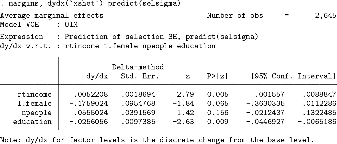
To further illustrate nehurdle‘s functionality, here is how to fit an exponential truncated hurdle model with heteroskedasticity in the selection equation: ⁹

By specifying the exponential option, nehurdle models the natural logarithm of the explained variable in the value equation. To specify that we want to model heteroskedasticity in the selection equation, we specify the het() option with the explanatory variables for the heteroskedasticity within the select() option. Notice that since we are using the same explanatory variables for the selection equation as for the value equation, we do not need to list them in the select() option. Just like with the standard deviation of the value equation, we can estimate the standard deviation of the selection equation by using margins with selsigma as the option to predict. Like before, we can get the APEs on the censored mean and on the standard deviation of the selection equation.

3.3 Type II tobit model

The type II tobit model assumes that the selection and value processes are different, like with the truncated hurdle model, but not independent. In our case, altruism and donations are not independent. We keep assuming that uncensored donations are still generated by the process in (1) and that altruism is generated by the process in (2). We further assume that the unobserved characteristics of the uncensored donations, u_i , and the unobserved characteristics of altruism, v_i , are not independent from each other. They are, in fact, correlated by a constant factor ρ. In other words, u and v follow a bivariate normal distribution:

$\left(u, v\right)\sim N_{\text{2}}(0,0, {\sigma }_u, {\sigma }_v, \rho )$

This presents a problem when using a linear specification of the value equation. Because both altruism and donations are jointly determined, whether the person presents a positive donation should be determined in that joint process. There is no guarantee, however, that this is the case. We could have cases where altruism is positive and the person is willing to donate, but we still have negative uncensored donations because the person’s income is not large enough. This is illustrated in the following data generation:

We generate income and age in the usual way. To generate the error terms for both processes, selection and value, we use the command drawnorm, so we need to create the variance–covariance matrix for the binormal distribution, vcv. From before, we have that σ_u = 2 and σ_v = 1. Setting the correlation between the error terms to 0.6, then, we have ${\sigma }_u^2={\text{ 2}}^{\text{2}}=\text{ 4}$ and ${\sigma }_v^2={\text{ 1}}^{\text{2}}=\text{ 1}$ , and the covariance between the two variables is σ_uv = σ_u × σ_v × ρ = 2 × 1 × 0.6 = 1.2. Using the cov() option of drawnorm with vcv, we generate the two error terms, u and v, and then use them to generate dstar and altruism, respectively. The descriptive statistics of dstar for those observations where altruism is positive illustrate the issue. We see that the minimum value is negative, and thus we have negative values even though altruism is positive. We cannot use the type II tobit estimator in this case, and that is why Wooldridge (2010, sec. 17.6.3) explains that we should not use a linear type II tobit model with variables with corner solutions. Only in the case where altruism being positive always implies that the uncensored donation is positive can we use a type II tobit with a linear specification of the value equation. The question is: how can we be sure this is the case when we only observe the censored variable?

This is not a problem for an exponential specification of the value equation, because all uncensored donations will be positive, so overcoming the selection hurdle guarantees that the uncensored mean is positive. I thus present the estimation of an exponential type II tobit using the PSID data with heteroskedasticity in the value equation, to illustrate another nehurdle functionality.

We see that, to fit a type II tobit model, we need to specify the heckman option. The name of the option follows the common naming of this model in the sample selection literature, given that Heckman (1976, 1979) proposed a two-step estimator. This naming is so common that Stata’s command to fit sample selection models is named heckman. The fact that we are using an estimator that is commonly used to deal with sample selection does not mean that a variable with corner solutions is a case of sample selection—it is not. Having said that, the naming of the option for the type II tobit model should make it easier for Stata users to identify it.

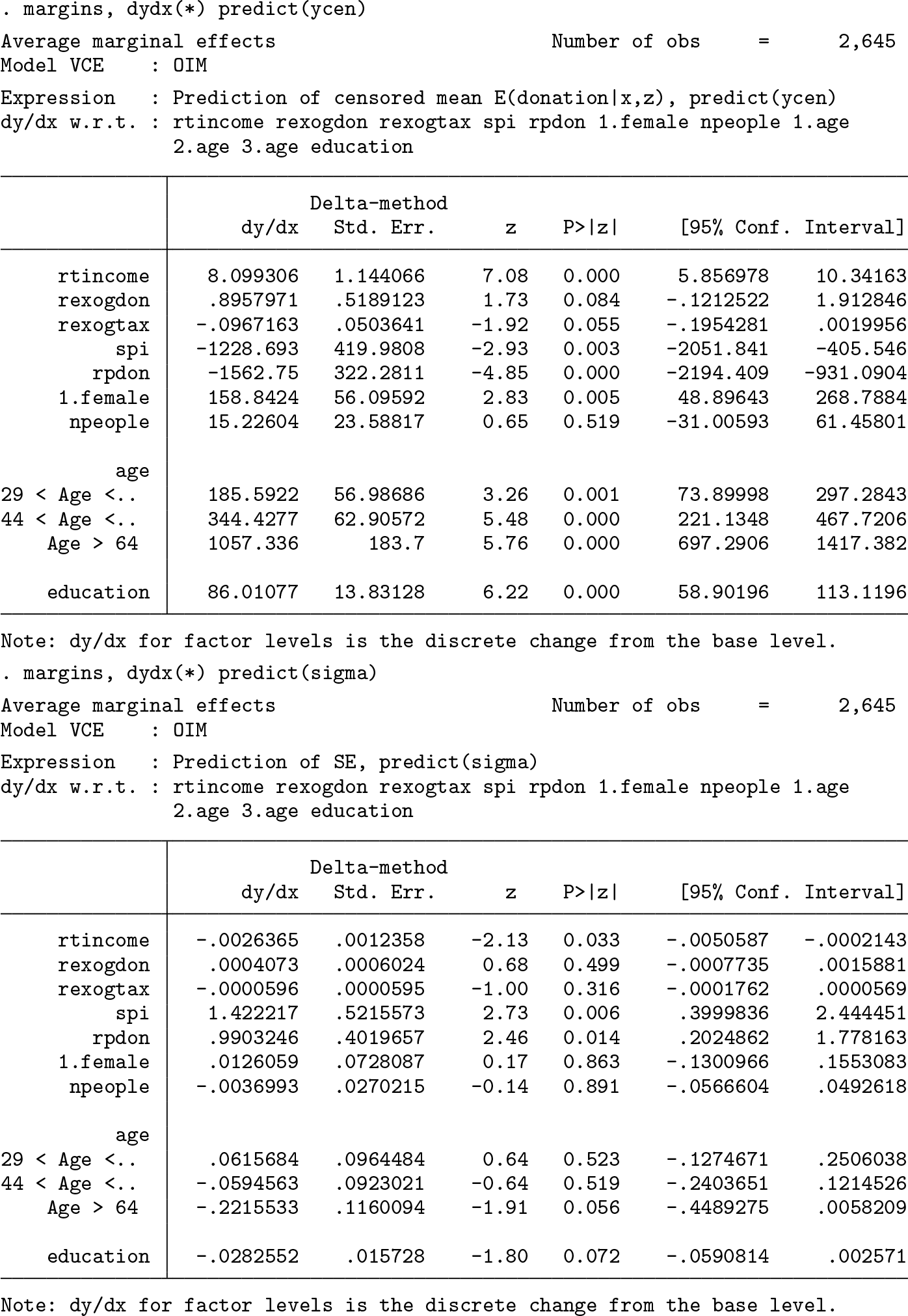
As we have seen before, we use the exponential option to specify the exponential value process and the het() option to specify the explanatory variables of the multiplicative heteroskedasticity of the value process. We then use margins to estimate the standard deviation of the value process by using the predict(sigma) option and the coefficient on the inverse Mills ratio, that is, the covariance between both processes, by using the predict(lambda)option. Our estimates indicate that the correlation between the two processes is significantly negative. We see that nehurdle actually estimates the inverse hyperbolic tangent of the correlation, as does the heckman command as well. To test whether the correlation is 0 or not, all we need is the test of individual significance of the inverse hyperbolic tangent of the correlation. The reason is that tanh(0) = 0, so if /athrho = 0, the correlation will also be 0.

Because we are estimating an exponential type II tobit with heteroskedasticity in the value equation, we can also estimate the APEs on the censored mean and on the standard deviation of the value process.

Clearly, you can also model heteroskedasticity in the selection equation in the same way we did in the estimation of the exponential truncated hurdle model.

In addition, and for completeness, nehurdle does allow for the estimation of a type II tobit model with a linear specification of the value function, but always keep in mind the previous discussion of the problems with that specification of the model.

4 Conclusions

In this article, I have introduced an estimation command, nehurdle, that estimates via maximum likelihood the three popular models used with variables with corner solutions: the tobit model, the truncated hurdle model, and the type II tobit model. I have explained the assumptions behind each estimator not only from a descriptive side, but also from a practical one by generating datasets for the homoskedastic linear specification of each model that follow their assumptions. In addition, I illustrated how to model heteroskedasticity in the value equation, and in the selection equation where appropriate, and to specify an exponential value equation. Furthermore, I illustrated with the use of margins how to get estimates of the partial effects on the censored mean and of the standard deviation of the appropriate equation when modeling heteroskedasticity. The partial effects on the censored mean are of particular importance with variables with corner solutions because what we actually observe is the censored variable, not the uncensored one.

Because the purpose of this article is to introduce the estimation command, I have only considered nehurdle‘s most important functionality. nehurdle is a byable command; that is, it can be used with the by prefix to do the same estimation across different groups or categories. It is also designed to be used with advanced survey techniques with the svy prefix. It provides other predict options than those presented here; the other options are documented in its help files.

Supplemental Material

Supplemental Material, st0550 - Estimation methods in the presence of corner solutions

Supplemental Material, st0550 for Estimation methods in the presence of corner solutions by Alfonso Sánchez-Peñalver in The Stata Journal

References

1.
CraggJ. G.1971. Some statistical models for limited dependent variables with application to the demand for durable goods. Econometrica39: 829–844.
2.
HeckmanJ. J.1976. The common structure of statistical models of truncation, sample selection, and limited dependent variables and a simple estimator for such models. Annals of Economic and Social Measurement5: 120–137. http://www.nber.org/chapters/c10494.
3.
HeckmanJ. J.1979. Sample selection bias as a specification error. Econometrica47: 153–161.
4.
TobinJ.1958. Estimation of relationships for limited dependent variables. Econometrica26: 24–36.
5.
WooldridgeJ. M.2010. Econometric Analysis of Cross Section and Panel Data. 2nd ed. Cambridge, MA: MIT Press.
Supplementary Material
Please find the following supplemental material available below.
For Open Access articles published under a Creative Commons License, all supplemental material carries the same license as the article it is associated with.
For non-Open Access articles published, all supplemental material carries a non-exclusive license, and permission requests for re-use of supplemental material or any part of supplemental material shall be sent directly to the copyright owner as specified in the copyright notice associated with the article.