Sage Journals: Discover world-class research

Abstract

Objective:

Accurate diagnosis of early Alzheimer disease (AD) plays a critical role in preventing the progression of memory impairment. We aimed to develop a new deep belief network (DBN) framework using 18F-fluorodeoxyglucose (FDG) positron emission tomography (PET) metabolic imaging to identify patients at the mild cognitive impairment (MCI) stage with presymptomatic AD and to discriminate them from other patients with MCI.

Methods:

18F-fluorodeoxyglucose-PET images of 109 patients recruited in the ongoing longitudinal Alzheimer’s Disease Neuroimaging Initiative study were included in this analysis. Patients were grouped into 2 classes: (1) stable mild cognitive impairment (n = 62) or (2) progressive mild cognitive impairment (n = 47). Our framework is composed of 4 steps: (1) image preprocessing: normalization and smoothing; (2) identification of regions of interest (ROIs); (3) feature learning using deep neural networks; and (4) classification by support vector machine with 3 kernels. All classification experiments were performed with a 5-fold cross-validation. Accuracy, sensitivity, and specificity were used to validate the results.

Result:

A total of 1103 ROIs were obtained. One hundred features were learned from ROIs using the DBN. The classification accuracy using linear, polynomial, and RBF kernels was 83.9%, 79.2%, and 86.6%, respectively. This method may be a powerful tool for personalized precision medicine in the population with prediction of early AD progression.

Keywords

Alzheimer disease PET prediction deep belief network

Introduction

Alzheimer disease (AD) is an insidious progressive neurodegenerative disease. It is also the most common type of senile dementia. Alzheimer disease mainly manifests as progressive memory disorder, cognitive disorder, personality change, and language disorder that seriously affects social, career, and life functions.¹ The etiology and pathogenesis of AD have not been elucidated; the characteristic pathological changes are tau hyperphosphorylated neurofibrillary tangles in nerve cells as well as neuronal loss with glial cell proliferation.²

The early diagnosis of AD is primarily associated with the detection of mild cognitive impairment (MCI), a prodromal stage of AD.^3,4 Although the memory complaints and deficits of MCI do not notably affect the patients’ daily activities, it has been reported that MCI has a high risk of progression to AD or other forms of dementia. The accurate early diagnosis of AD, especially identifying the risk of progression of MCI to AD, affords patients’ with AD awareness of the severity and allows them to take preventative measures.^5,6 Hence, predicting AD from MCI has an important clinical value.

18F-Fluorodeoxyglucose (FDG) positron emission tomography (PET) measures the decline in the regional cerebral metabolic rate of glucose, offering a reliable metabolic biomarker even in patients with presymptomatic AD because the regional metabolic aberration underlies the functional and cognitive decline seen in patients with AD.⁷ Positron emission tomography scans provide functional information that is unique and unavailable using other types of imaging. Hence, 18F-FDG-PET is recognized as a potential tool for presymptomatic diagnosis of AD, offering acceptable sensitivity and accuracy.⁸ The analysis of 18F-FDG-PET based on artificial intelligence, such as machine learning and deep learning, has gradually become mainstream.⁹

For example, Zhang¹⁰ et al used Multiple Kernel Learning to build a classifier for MCI and normal group (NC), which was further used to classify MCI converters and nonconverters. Two imaging modalities, nuclear magnetic resonance imaging (MRI) and FDG-PET, were used together with 1 non-imaging modality, cerebrospinal fluid (CSF) measurements. Young¹¹ et al proposed building an AD versus NC classifier using a Gaussian process, which was then used to classify MCI converters and nonconverters. Wang¹² et al proposed 2 partial least squares–based approaches to classify MCI converters and nonconverters using MRI, FDG-PET, and florbetapir PET.

Additionally, with the development of deep learning, a few deep neural networks have also been applied to recognize AD-related progression patterns. Lu¹³ et al proposed a multiscale deep neural network–based deep belief network (DBN) for classification using measures from a single modality. Liu¹⁴ et al constructed a cascaded convolutional neural network to learn the multilevel and multimodal features of MRI and PET brain images. Suk¹⁵ et al used a deep learning–based latent feature representation with a stacked autoencoder (SAE) by using MRI, FDG-PET, and CSF data. They also¹⁶ found a novel method for a high-level latent and shared feature representation from neuroimaging modalities via deep learning; they used Deep Boltzmann Machine (DBM), found a latent hierarchical feature representation from a 3-dimensional (3D) patch, and then devised a systematic method for a joint feature representation from the paired patches of MRI and PET with a multimodal DBM.

However, these existing methods have limitations. Most of these attempts toward developing automated tools to identify progressive MCI have resulted in limited accuracy (less than 80%). Therefore, the present study aimed to propose a novel framework with a deep neural network based on DBN, which can effectively learn the patterns of metabolic changes between MCI converters and nonconverters using FDG-PET images.

Materials and Methods

As shown in Figure 1, the proposed framework is composed of 4 steps: (1) image preprocessing, including normalization and smoothing; (2) identification of regions of interest (ROIs); (3) feature learning, including unsupervised pretraining in DBN and supervised fine-tuning in back-propagation (BP) network; and (4) discrimination of MCI-to-AD converters from patients with normal MCI using support vector machine (SVM).

Figure 1.

The workflow in this analysis was composed of 4 steps: image preprocessing, obtaining regions of interest, feature learning, and support vector machine (SVM) classification.

Materials

Data for this article were obtained from the publicly available Alzheimer’s Disease Neuroimaging Initiative (ADNI) database¹⁷ (http://adni.loni.usc.edu). The ADNI was launched in 2003 as a public–private partnership, led by principal investigator Michael W. Weiner, MD, VA Medical Center and University of California San Francisco. Patients were recruited from over 50 sites across the United States and Canada. This multisite open-source data set was designed to accelerate the discovery of biomarkers and to identify and track AD pathology. For up-to-date information, see http://www.adni-info.org.

Participants (n = 109) were evaluated at baseline and in 6- to 12-month intervals following initial evaluation for up to 10 years. 18F-fluorodeoxyglucose-PET scans acquired at the baseline visit were used in the present analysis. We included the patients who were diagnosed with MCI and had a Mini-Mental State Examination (MMSE) score of at least 24 points at the time of PET imaging. Additionally, we requested a minimal follow-up time of at least 6 months. The patients were stratified into patients with MCI who converted to AD (MCI-to-AD converters, progressive mild cognitive impairment [pMCI]) and those who did not (MCI nonconverters, stable mild cognitive impairment [sMCI]).

The PET data acquisition details can be found online in the study protocols of the ADNI project. Images were acquired 30 to 60 minutes after the injection. Age, sex, and MMSE did not differ significantly between the 2 groups (P > .1). Demographic and clinical information of these patients are described in Table 1.

Table 1.

Patient Demographics.

Group	Gender, M/F	Age, Years	Conversion, Month	MMSE Score
pMCI (n = 47)	27/20^a	73.3 ± 7.1^a	/	27.1 ± 1.2^a
sMCI (n = 62)	38/24^a	75.8 ± 6.1^a	12.2 ± 4.38	27.8 ± 1.4^a

Abbreviations: AD, Alzheimer disease; MCI, mild cognitive impairment; MMSE, Mini-Mental State Examination; pMCI, progressive mild cognitive impairment; sMCI, stable mild cognitive impairment.

^a t test, P > .1.

Image Preprocessing

Image data were processed using statistical parametric mapping (SPM8; http://www.fil.ion.ucl.ac.uk/spm/) implemented in MATLAB R2014b.¹⁸

The aim of preprocessing was to spatially normalize the images into Montreal Neurological Institute (MNI) space. The image preprocessing was composed of 2 steps: normalization and smoothing. All original DICOM data were converted to the NIfTI format file using dcm2nii. For every patient, their images were spatially normalized to the standard MNI space provided by SMP8 with linear and nonlinear 3D transformations. After that, the normalized images had a spatial resolution of 91 × 109 × 91 with a 2 × 2 × 2 mm³ voxel size. Finally, normalized FDG images were smoothed using an isotropic Gaussian smoothing kernel with a full-width at half-maximum of 10 × 10 × 10 mm³.

Region of Interest

In our study, a region-growing algorithm¹⁹ is set to extract spatially constrained atoms in whole brain images to reduce the computational burden. These ROIs in the sample series are composed of voxels whose series share some similarity; some regions are homogeneous while some are heterogeneous. We therefore aim to segment the brain cortex into a set of disjoint regions, each being a set of voxels connected with respect to its 26-connexity; the resulting regions are homogeneous in the whole series. This is achieved by means of a competitive region-growing algorithm, which is an iterative procedure for image segmentation.

This procedure starts from small regions, in our case, the set of all singletons of voxels in the PET images, which grow simultaneously at each step by merging with other neighboring voxels or regions on the basis of similarity criteria.

Because similarity is measured through correlation, we chose to measure the similarity between 2 regions as the mean correlation between the series of any 2 voxels, each belonging to a different region. The similarity measure between 2 regions is as follows:

s (C, D) = \frac{1}{# C # D} \sum_{v, w \in C \times D} corr (y_{v}, y_{w}),

where corr is Pearson linear correlation, #C is the number of voxels in region C, and $y_{v}$ is the series of voxel v, $y_{w}$ is the series of voxel w.

For a single voxel v, the neighborhood is defined N(v), which is the 26-connected neighborhood for v. The neighborhood of region C can be defined as follows:

N_{n} (C) = D \in E_{n}, D \neq C | \exists (v, w) \in C \times D, w \in N (v),

where E_n are candidates for merging in step n. Since all regions compete at each step for merging, it is necessary to define a merging rule.

We used the mutual nearest neighbor principle,²⁰ which is designed to merge the most similar regions at first. A pair of neighboring regions, such as C and D, will merge if it fulfills the following condition:

mnn (C, D) \Leftrightarrow {\begin{matrix} C = \underset{K \in N_{n} (D)}{arg min} s (K, D) \\ a n d \\ D = \underset{L \in N_{n} (C)}{arg min} s (C, L) \end{matrix} .

The algorithm stops when all regions have reached the critical size or when additional merging is not possible.

In this analysis, according to the algorithm, all 3D 18F-FDG-PET images in the training data set were stacked along a fourth (subject) dimension (4D), creating a single 4D image to be used in the region-growing algorithm, which was set to extract spatially constrained atoms with a size threshold of 1000 mm³. To limit the memory demand, the region-growing algorithm was applied independently in each of the 116 areas of the anatomical automatic labeling (AAL) template.²¹

Feature Learning

Hinton et al²² reported that deep supervised nets can be trained by adding an unsupervised pretraining by restricted Boltzmann machine (RBM) for parameter initialization. In the deep learning model, with a relatively small number of training samples, the DBN, which was stacked with RBMs, has certain advantages.²³

A DBN is a deep architecture that is suitable for delivering nonlinear and complicated machine-learning information. A DBN model is actually a multilayer perception neural network with 1 input layer, 1 output layer, and several middle-hidden layers unit. The higher level layer connects to its lower layer by RBM,²⁴ which uses the result of the lower layer to activate the next higher level layer. For DBN, the training contains 2 steps, unsupervised pretraining and supervised fine-tuning.

Unsupervised pretraining

First, the model is pretrained as an SAE. The autoencoder acts as an unsupervised concept extractor for the original data samples. It learns the latent representation in the hidden layer (encoder) and reconstructs the data in the output layer (decoder). The core of this step is RBM.

Restricted Boltzmann machine is based on the assumption²⁵ of the Boltzmann distribution between observed and hidden variables generalized to Gaussian distributions, which setup the foundation of our model.

A simple RBM is composed of a visible layer and a hidden layer. The visible layer has m nodes, ${v_{1}, v_{2} \dots v_{m}}$ . The hidden layer has n nodes, ${h_{1}, h_{2} \dots h_{n}}$ . ${b_{1}, b_{2} \dots b_{n}}$ and ${c_{1}, c_{2} \dots c_{n}}$ are the bias of each node, and w is the weight value between nodes.

For pairwise training between nodes of input layers and hidden layers, a conditional Gaussian distribution is used:

P_{p} (h_{j} = 1 | v) = sig (c_{j} + \sum_{i = 1}^{m} v_{j} w_{i j}) .

P_{p} (v_{i} = 1 | h) = sig (b_{j} + \sum_{j = 1}^{n} h_{j} w_{i j}),

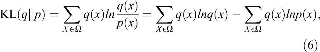
where sig is the logistic function: $sig (x) = \frac{1}{1 + e^{- x}}$ . The KL distance between the sample distribution and the edge distribution of the RBM network can represent the difference between them:

KL (q | | p) = \sum_{X \in Ω} q (x) l n \frac{q (x)}{p (x)} = \sum_{X ϵ Ω} q (x) l n q (x) - \sum_{X ϵ Ω} q (x) l n p (x),

where Ω is the sample space, q is the distribution of input samples, q(x) is the probability of the training sample, and P is the edge distribution represented by the RBM network. We minimize the KL to fit the training data during training progress.

Supervised fine-tuning

Because the deep network is prone to local optimization, the choice of initial parameters has a great impact on the final convergence location of the network. Therefore, DBN training is divided into pretraining and fine-tuning.

The parameters trained by DBN are used to initialize a BP network with the same structure. Back-propagation network adopted a gradient descent algorithm to fine-tune the weight of the whole network to coordinate and optimize the parameters of the whole DBN. The feature vector mapping of the DBN is optimized, and the size of the input apace is simplified.

We take some measures to reduce chances of overfitting during training progress—(1) Dropout strategy²⁶: Dropout is a popular strategy to prevent overfitting. We choose the percentage of units kept to feed to the next layer. For training, half of the hidden units were dropped randomly in each iteration, while the other half were retained to feed features to the next layer. For testing, all the units were kept to classify patients. (2) Regularization strategy²⁷: The purpose of adding regularization terms is to reduce the error of the test set at the cost of increasing the error of the training set. Because in the case of a small amount of data, if the training set error is small, it may appear overfitting. L2 regularization is used in this analysis to reduce the summation of parameters squared.

Classification of SVM

To perform classification tasks, we use a model such as SVM²⁸ to replace the traditional SoftMax function in DBN²⁹ because SVM achieves maximum margin classification in the training data set. Additionally, SVM is a more powerful model when the kernel function is adjusted to support nonlinear mapping. The input of the SVM is the result of feature coding of the original regions ROIs by the DBN. In the classification experiment, 3 kernel functions (linear, polynomial, and radial basis) were used for detecting features’ generalization ability and classification reliability.

Comparison Experiments

Two shallow models are applied for comparison. The first one is a standard SVM without deep architecture-based feature learning. We use the average metabolism of 90 regions extracted from the standard AAL template as the SVM feature input. For the second model, we use principle component analysis (PCA) for feature extraction. In the training set, we used PCA to reduce the dimension of ROIs obtained by the region growth algorithm. The number of PCA eigenvectors was chosen to retain 95% variance, and the feature after dimension reduction was used as the feature input of SVM.

Three different kernel functions were used in SVM. A 5-fold cross-validation method is used for classification. The accuracy, sensitivity, and specificity are used to evaluate the model performance.

Results

Region of Interest

According to this competitive region-growing algorithm, we finally obtain 1103 ROIs, as shown in Figure 2. Although voxels in these regions in the series are similar, for 2 types of samples, pMCI and sMCI, some regions are heterogeneous and some are homogeneous. These ROIs may offer enhanced clinical utility by utilizing information specific to PET signals.

Figure 2.

The 1103 regions of interest (ROIs) extracted from the region-growing algorithm.

Figure 3 shows the average of standardized uptake value ratio of samples in all ROIs. Each column represents a single sample, and each row represents the same ROI from the region-growing algorithm. In addition, we observed from the figure that in some ROIs, the average metabolism of the 2 types of samples was significantly different. This proves that some ROIs we extracted were heterogeneous, which can reflect the difference between pMCI samples and sMCI samples.

Figure 3.

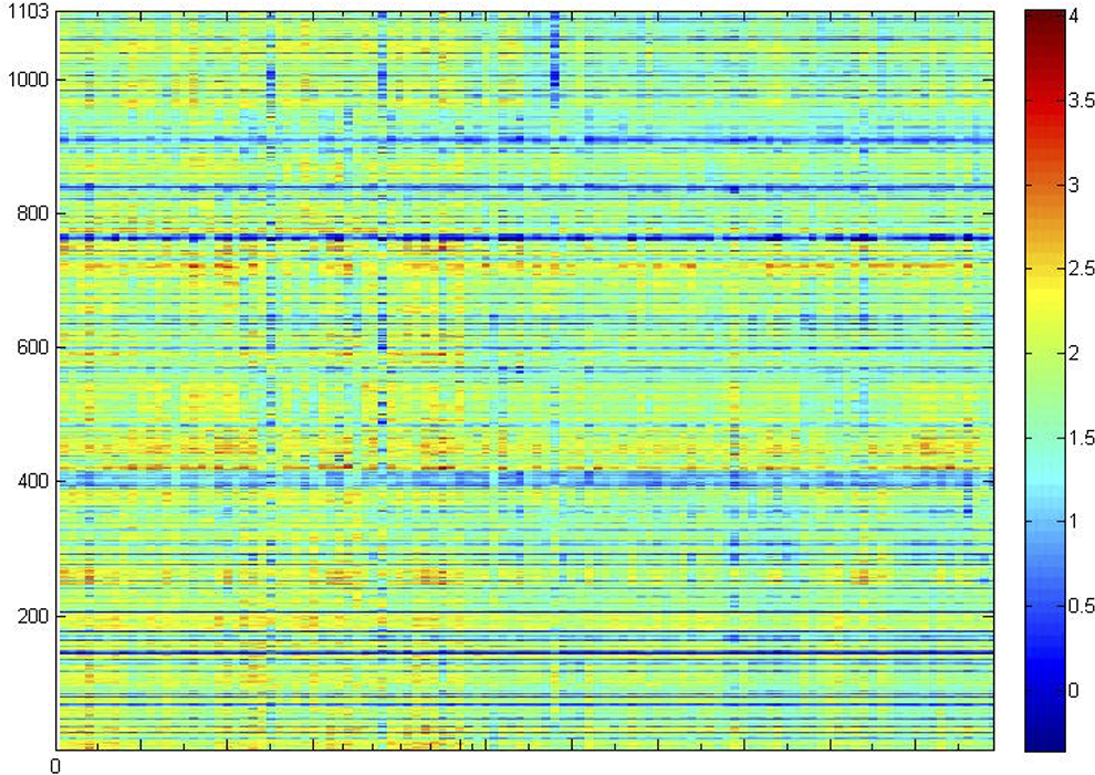
Average of standardized uptake value ratio of samples in all regions of interest (ROIs).

Feature Learning

Age, sex, and MMSE did not differ significantly between the 2 data sets as shown in Table 1; we propose DBN as the main deep model for feature learning in this study. We use metabolism features in ROIs as input of our single-mode DBN. The output is the result of relearning the features. We aim to preserve the original features as much as possible while reducing the dimensions of features. Thus, the essence of the DBN is the process of feature learning, that is, achievement of enhanced feature expression.³⁰

Our deep model is shown in Figure 4. First, a DBN stacked by 3 RBMs was used for feature dimension reduction and recoding like an autoencoder. The input feature dimension is 1103 (the number of ROIs), and the output feature dimension is 100. For each layer, the number of nodes is 1000, 500, 500, and 100. Then, the trained parameters of DBN were used to initialize a BP network with the same structure, and the parameters of last hidden layer are the last extracted features.

Figure 4.

Deep belief network for feature learning.

All the training steps shared the same BP approach. The cost function was minimized using gradient descent with mini-batches³¹; the training set was randomly divided into several mini-batches, or subsets, with 5 samples in each batch. In each iteration, only one of these mini-batches was used for minimization. After all the samples were used once for training, the training set was ordered and divided again so that batches in each different echo will not have the same samples. The initial learning rate was set to 0.001.

We used training cost and accuracy of final SVM classification to measure the deep feature learning model. As shown in Figure 5, we found that when the number of network epoch increased, the accuracy of classification rise, and the training cost decreased. When the number of epochs achieved 90, the cost and accuracy gradually tend to be stable. Hence, we choose 90 epochs in our experiments.

Figure 5.

The influence of the number of epochs on the accuracy and cost of classification in deep belief network (DBN).

Classification of SVM

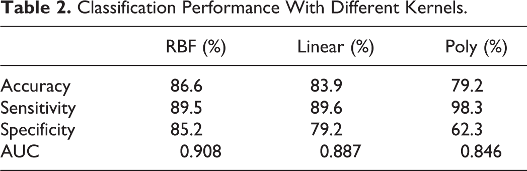
The mean accuracy, sensitivity, and specificity of the cross-validation experiment are shown in Figures 6 and 7 and Table 2. In the classification experiment, using features from the DBN with radial basis, kernel, linear, and polynomial achieved accuracies of 86.6%, 83.9%, and 79.2%, respectively, to distinguish MCI-to-AD converters from stable patients with MCI. As a result, classification experiment with RBF kernel has best accuracy, specificity, and area under the curve (AUC) value.

Figure 6.

Receiver operating characteristic (ROC) curves with different kernels.

Figure 7.

Receiver operating characteristic (ROC) curves with 5-fold cross validation.

Table 2.

Classification Performance With Different Kernels.

	RBF (%)	Linear (%)	Poly (%)
Accuracy	86.6	83.9	79.2
Sensitivity	89.5	89.6	98.3
Specificity	85.2	79.2	62.3
AUC	0.908	0.887	0.846

Comparison Experiment

The results of the comparison experiment are shown in Figure 8 and Table 3. As a comparison, the classification accuracy of the combination of PCA and SVM and AAL and SVM was 79.5% and 63.1%, respectively. As we can see from the Table 3, ROIs extracted by the region-growing algorithm better reflects the differences compared to the AAL template; compared to traditional PCA, DBN has better feature extraction capability. The DBN shows more profound feature information through layer-by-layer feature transformation and extraction, overcoming the fact that PCA cannot extract nonlinear information.

Figure 8.

Receiver operating characteristic (ROC) curves of the comparison experiment.

Table 3.

Classification Performance of the Comparison Experiment.

	Accuracy, %	Sensitivity, %	Specificity, %
AAL + SVM	63.1	84.1	24.2
PCA + SVM	79.5	76.2	80.2
DBN + SVM	86.6	89.5	85.1

Abbreviations: AAL, anatomical automatic labeling; DBN, deep belief network; PCA, principle component analysis; SVM, support vector machine.

Discussion

In this study, we achieved an 86% accuracy to predict AD from MCI, which is a better result than others reported in the literature. Table 4 shows the results from current methods to predict the conversion of MCI. Although the data used in different studies are not identical, they all come from the ADNI database; therefore, they share a similar acquisition and preprocessing procedure, allowing comparisons to be made.

Table 4.

Classification Performance of the Published State-of-the-Art Methods.

Reference	Modality	Patients	Accuracy	Sensitivity	Specificity
Zhang¹⁰ et al, 2011	PET + MRI + CSF	80	73.9	68.6	73.6
Young¹¹ et al, 2013	MRI + PET + APOE	143	69.9	78.7	65.6
Wang¹² et al, 2016	PET + MRI + ADAS	129	86.1	81.3	90.7
Liu³² et al, 2017	PET + MRI	234	73.5	76.19	70.37
Cheng⁵ et al, 2017	PET + MRI + CSF	99	79.4	84.5	72.7
Zhu³³ et al, 2015	PET + MRI	99	72.4	49.1	94.6
Lu¹³ et al, 2018	PET + MRI	521	81.55	73.33	83.83
Lu¹³ et al, 2018	PET	626	81.53	78.20	82.47
Suk¹⁶ et al, 2015	PET + MRI + CSF	99	83.3	–	–
Proposed method	PET	109	86.6	89.5	85.2

Abbreviations: CSF, cerebrospinal fluid; MRI, magnetic resonance imaging; PET, positron emission tomography; ADAS, alzheimer's disease assessment scale; APOE, apolipoprotein E.

As shown in Table 4, we achieved the best results in accuracy and sensitivity and achieved almost the best results in specificity. Possible reasons include the following:

For the extraction of ROIs, we use a competitive region growth algorithm to extract ROI. In the study by Lu¹³ et al, the voxels in each ROI were clustered into patches through k-means clustering based on the Euclidean distance of their spatial coordinates, which means that voxels spatially close to each other would belong to the same patch. Suk¹⁵ et al performed a 2-sample t test on each voxel, selected voxels with a P value smaller than the predefined threshold, and extracted patches as ROIs with a fixed size by taking each of these voxels as a center. The results show that the ROIs extracted through our method have greater differences. We obtain the ROIs with spatial coordinates according to Pearson correlation of the sample series, which can reflect better differences between samples than single voxel or the ROIs obtained based on the Euclidean distance.

In terms of feature learning, we adopted an improved DBN model that reduces the complexity of the whole prediction algorithm while using single modality data. A DBN adopts the training and fine-tuning mode of training, which means that unsupervised pretraining can help deep learning find better optimal parameters for reducing errors, effectively avoiding the problem of parameter selection. Therefore, only a small amount of a sample can train a good classifier using a DBN, which has obvious advantages in the recognition of a small sample.

For the classification, we use SVM for classifiers to replace SoftMax in last layer of BP network because SVM has prominent advantages in solving the problem of identifying small samples.

Although our method based on a single modality can guarantee a high level of specificity, accuracy, and sensitivity, some limitations and disadvantages also exist in our method:

Due to the limited data in the ADNI database, we only used a limited data set, so the network structure used in our experiment to discover information from MCI is not necessarily suitable for other data sets. Also, the number of cases in this study appeared not much for a current AI learning, and it is still not enough to generalize our experimental results. We need more in-depth research, such as learning the optimal network structure from big data, for a practical application of deep learning in clinical scenarios.

Many other modality characteristics in the ADNI data set, such as clinical information, age, education, and CSF parameters, are not used, and it is still necessary to design a multimodal deep learning network to learn potential relationships among features from multiple modalities.

There is no general and intuitive way to visualize the training weights or interpret the underlying characteristics. Effectively visualizing or interpreting the representation of potential features is a major challenge that needs to be addressed by both machine learning and the clinical neuroscience community.

Conclusion

In this study, a new framework for the early diagnosis of AD using DBN to extract the features of FDG-PET data is proposed. The framework improves the performance of deep neural networks in identifying sMCI and pMCI objects by using the strategy of extracting high-dimensional difference ROIs in advance. Experiments in the FDG-PET image database of 109 patients provided evidence to support 2 assertions: (1) The proposed method, which uses only features derived from a single FDG-PET modality, can be superior to existing methods that use multimodal features in the sMCI versus pMCI classification task; (2) the proposed network can learn the discriminant mode from the difference ROIs to obtain a more robust classifier with better discriminant performance. We argue, therefore, that the proposed method can be a powerful means to represent neuroimaging biomarkers for the early diagnosis and prediction of AD populations.

Footnotes

Author Contribution

Ting Shen and Jiaying Lu equally contributed to this work.

Declaration of Conflicting Interests

The author(s) declared no potential conflicts of interest with respect to the research, authorship, and/or publication of this article.

Funding

The author(s) disclosed receipt of the following financial support for the research, authorship, and/or publication of this article: This study was supported by grants from the National Natural Science Foundation of China (No. 61603236, No. 81671239, No. 81361120393, No. 81401135), the Shanghai Technology and Science Key Project in Healthcare (No.17441902100), the Shanghai National Science Foundation (18ZR1405400, 17ZR1427700), the Key Project in Healthcare (No. 17441902100), and the Shanghai Sailing Program (16YF1415400).

ORCID iD

Jiehui Jiang

References

Alzheimer’s Association. 2013 Alzheimer’s disease facts and figures. Alzheimers Dement. 2013;9(2):208–245.

Grundman

Petersen

Ferris

, et al. Mild cognitive impairment can be distinguished from Alzheimer disease and normal aging for clinical trials. Arch Neurol. 2004;61(1):59–66.

Morris

Storandt

Miller

, et al. Mild cognitive impairment represents early-stage Alzheimer disease. Arch Neurol. 2001;58(3):397–405.

Bennett

Schneider

Bienias

Evans

Wilson

. Mild cognitive impairment is related to Alzheimer disease pathology and cerebral infarctions. Neurology. 2005;64(5):834.

Cheng

Zhang

Shen

. Domain transfer learning for mci conversion prediction. IEEE Trans Biomed Eng. 2015;62(7):1805–1817.

Davatzikos

Bhatt

Shaw

Batmanghelich

Trojanowski

. Prediction of mci to ad conversion, via MRI, CSF biomarkers, and pattern classification. Neurobiology of Aging. 2011;32(12):2322.e19–e27.

Chételat

Desgranges

Sayette

VDL

Viader

Eustache

Baron

. Mild cognitive impairment can FDG-pet predict who is to rapidly convert to Alzheimer’s disease? Neurology. 2003;60(8):1374–1377.

Smailagic

Lafortune

Kelly

Hyde

Brayne

. 18f-FDG pet for prediction of conversion to Alzheimer’s disease dementia in people with mild cognitive impairment: an updated systematic review of test accuracy. J Alzheimers Dis. 2018;64(4):1175–1194.

Liu

Chen

Weidman

Lure

. Use of multimodality imaging and artificial intelligence for diagnosis and prognosis of early stages of Alzheimer’s disease. Transl Res. 2018;194:56–67.

10.

Zhang

Wang

Zhou

Yuan

Shen

. Multimodal classification of Alzheimer’s disease and mild cognitive impairment. Neuroimage. 2011;55(3):856–867.

11.

Young

Modat

Cardoso

Mendelson

Cash

Ourselin

. Accurate multimodal probabilistic prediction of conversion to Alzheimer’s disease in patients with mild cognitive impairment. Neuroimage Clinical. 2013;2(1):735–745.

12.

Wang

Chen

Yao

, et al. Multimodal classification of mild cognitive impairment based on partial least squares. J Alzheimers Dis. 2016;54(1):359–371.

13.

Popuri

Ding

Balachandar

Beg

. Multimodal and multiscale deep neural networks for the early diagnosis of Alzheimer’s disease using structural MR and FDG-PET images. Sci Rep. 2018;8(1):5697.

14.

Liu

Cheng

Wang

. Multi-modality cascaded convolutional neural networks for Alzheimer’s disease diagnosis. Neuroinformatics. 2018;16(3-4):295–308.

15.

Suk

Lee

Shen

. Hierarchical feature representation and multimodal fusion with deep learning for AD/MCI diagnosis. Neuroimage. 2014;101:569–582.

16.

Suk

Lee

Shen

. Latent feature representation with stacked auto-encoder for AD/MCI diagnosis. Brain Struct Funct. 2015;220(2):841–859.

17.

Weiner

Veitch

Aisen

, et al. 2014 update of the Alzheimer’s Disease Neuroimaging Initiative: a review of papers published since its inception. Alzheimers Dement. 2015;11(6):e1–e120.

18.

Lange

Suppa

Frings

Brenner

Spies

Buchert

. Optimization of statistical single subject analysis of brain FDG pet for the prognosis of mild cognitive impairment-to-Alzheimer’s disease conversion. J Alzheimers Dis. 2016;49(4):945–959.

19.

Bellec

Perlbarg

Jbabdi

, et al. Identification of large-scale networks in the brain using fMRI. Neuroimage. 2006;29(4):1231–1243.

20.

Gowda

. Disaggregative clustering using the concept of mutual nearest neighborhood. Pattern Recognition. 1978;10(2):105–112.

21.

Tzourio-Mazoyer

Landeau

Papathanassiou

, et al. Automated anatomical labeling of activations in SPM using a macroscopic anatomical parcellation of the MNI MRI single-subject brain. Neuroimage. 2002;15(1):273–289.

22.

Hinton

Osindero

Teh

. A fast learning algorithm for deep belief nets. Neural Computation. 2006;18(7):1527–1554.

23.

Tolstikov

Biswas

Nugent

Parente

. Comparison of fusion methods based on DST and DBN in human activity recognition. Control Theory and Technology. 2011;9(1):18–27.

24.

Roux

Bengio

. Representational power of restricted Boltzmann machines and deep belief networks. Neural Computation. 2008;20(6):1631–1649.

25.

Welling

Teh

. Bayesian learning via stochastic gradient Langevin dynamics. International Conference on International Conference on Machine Learning. Bellevue, Washington, USA, 28 June - 2 July, 2011:681–688. Omnipress.

26.

Srivastava

Hinton

Krizhevsky

Sutskever

Salakhutdinov

. Dropout: a simple way to prevent neural networks from overfitting. J Mach Learn Res. 2014;15(1):1929–1958.

27.

Vincent

Larochelle

Lajoie

Bengio

Manzagol

. Stacked denoising autoencoders: learning useful representations in a deep network with a local denoising criterion. J Mach Learn Res. 2010;11(12):3371–3408.

28.

Suykens

JAK

Gestel

Brabanter

Moor

Vandewalle

. Least squares support vector machines. Int J Circuit Theory Appli. 2015;27(6):605–615.

29.

Liang

Zhang

Huang

. Deep learning for healthcare decision making with EMRs. IEEE International Conference on Bioinformatics and Biomedicine. Washington, USA, 9-12 November, IEEE; 2015:556–559.

30.

Hinton

Salakhutdinov

. Reducing the dimensionality of data with neural networks. Science. 2006;313(5786):504–507.

31.

Bengio

Practical Recommendations for Gradient-Based Training of Deep Architectures. Neural Networks: Tricks of the Trade. Berlin Heidelberg: Springer; 2012.

32.

Liu

Chen

Yao

Guo

. Prediction of mild cognitive impairment conversion using a combination of independent component analysis and the cox model. Front Hum Neurosci. 2017;11:33.

33.

Zhu

Suk

Wang

Lee

Shen

. A novel relational regularization feature selection method for joint regression and classification in ad diagnosis. Med Image Anal. 2017;38:205–214.

Predicting Alzheimer Disease From Mild Cognitive Impairment With a Deep Belief Network Based on 18F-FDG-PET Images

Abstract

Objective:

Methods:

Result:

Keywords

Introduction

Materials and Methods

Materials

Image Preprocessing

Region of Interest

Feature Learning

Unsupervised pretraining

Supervised fine-tuning

Classification of SVM

Comparison Experiments

Results

Region of Interest

Feature Learning

Classification of SVM

Comparison Experiment

Discussion

Conclusion

Footnotes

Author Contribution

Declaration of Conflicting Interests

Funding

ORCID iD

References