Sage Journals: Discover world-class research

Abstract

This article describes a macroscopic mathematical modeling approach to capture the interplay between solid tumor evolution and cell damage during radiotherapy. Volume regression profiles of 15 patients with uterine cervical cancer were reconstructed from serial cone-beam computed tomography data sets, acquired for image-guided radiotherapy, and used for model parameter learning by means of a genetic-based optimization. Patients, diagnosed with either squamous cell carcinoma or adenocarcinoma, underwent different treatment modalities (image-guided radiotherapy and image-guided chemo-radiotherapy). The mean volume at the beginning of radiotherapy and the end of radiotherapy was on average 23.7 cm³ (range: 12.7-44.4 cm³) and 8.6 cm³ (range: 3.6-17.1 cm³), respectively. Two different tumor dynamics were taken into account in the model: the viable (active) and the necrotic cancer cells. However, according to the results of a preliminary volume regression analysis, we assumed a short dead cell resolving time and the model was simplified to the active tumor volume. Model learning was performed both on the complete patient cohort (cohort-based model learning) and on each single patient (patient-specific model learning). The fitting results (mean error: ∼16% and ∼6% for the cohort-based model and patient-specific model, respectively) highlighted the model ability to quantitatively reproduce tumor regression. Volume prediction errors of about 18% on average were obtained using cohort-based model computed on all but 1 patient at a time (leave-one-out technique). Finally, a sensitivity analysis was performed and the data uncertainty effects evaluated by simulating an average volume perturbation of about 1.5 cm³ obtaining an error increase within 0.2%. In conclusion, we showed that simple time-continuous models can represent tumor regression curves both on a patient cohort and patient-specific basis; this discloses the opportunity in the future to exploit such models to predict how changes in the treatment schedule (number of fractions, doses, intervals among fractions) might affect the tumor regression on an individual basis.

Keywords

tumor mathematical modeling uterine cervical cancer radiosensitivity linear-quadratic model image-guided radiotherapy

Introduction

In the fight against cancer, radiotherapy represents a highly effective localized treatment, in which image-guidance (image-guided radiotherapy [IGRT]) plays a key role.^1,2 Morphologic images, as computed tomography (CT), cone-beam CT (CBCT), and magnetic resonance (MR), featuring diagnostic quality are acquired daily, in order (1) to check the occurrence of anatomical changes, (2) to adjust patient setup, and (3) to evaluate the need for treatment replanning and adaptive approaches (plan of the day).^3
-5 Functional imaging is applied as well to visualize tumor features (eg, glucose consumption, hypoxia, and repopulation), assess tumor staging, and predict the response to treatment.^6,7 According to the excellent review by Jadon et al,⁵ image guidance allows the evaluation of tumor volume along the radiotherapy course. Such extensive information can be in principle fruitfully exploited in the mathematical modeling of tumor response to therapy and toxicity effects on healthy tissues, thus allowing the simulation of a customized therapeutic plan.^7
-9 Modeling, ranging from simple tumor control probability (TCP) functions to multiscale mechanistic/phenomenological approaches of cell proliferation and invasion, has the potential to become a powerful tool to support clinical decision. In the framework of IGRT, the role of image processing and analysis is to link theoretical growth/therapy response models to macroscopic tumor changes, thus representing phenomenological features that cannot be observed directly.

Mathematical models have attempted to simulate the biological mechanism underlying the spatiotemporal growth of tumors and response to radiation and drugs. Time-discrete models at cell and tissue scales using the principle of cellular automata have been developed and applied to study a variety of radiobiological problems.^9

-12 In general, while sophisticated models may be able to represent biological phenomena more realistically, they can be hardly applied in the clinics, since the morphological and the functional information derived from medical images is difficult to include. Conversely, simpler time-continuous models at the tissue scale representing tumor growth, under conditions of mechanical pressure, nutrient shortage, and even therapeutic irradiation, can be directly compared to macroscopic measurements from clinical images.^8,13,14 Spatial effects are not taken into account and the tumor is assumed to include identical cells. Such simplification allows the model to be customized to patient subclasses or even for single patients. For example, exponential, logistic, or Gompertzian growth curves have been used to describe tumor repopulation during fractioned radiotherapy both in early¹⁵ and more recent works.^14,16,17 Most of such studies focused on simulated experiments and the potential of translation to clinical practice was not verified. Outcomes of the more recent articles turned out to grant sufficient descriptive power of tumor growth prior to therapy, finding a high correlation between tumor proliferation and radiosensitivity.¹⁴ However, further investigation seems mandatory to study the interplay between the response to radiation and the tumor repopulation along the course of a radiotherapy treatment in vivo.

In this article, we focused on macroscale, time-continuous mathematical approaches to represent the tumor cell killing effect due to radiation therapy and the concurrent repopulation, by integrating the linear-quadratic (LQ) and the Gompertzian/logistic tumor growth models. Volume regression profiles of patients with uterine cervical cancer were reconstructed from serial CBCT data sets, acquired for IGRT, and exploited for model parameter learning by means of a genetic-based optimization. Patients, diagnosed with either squamous cell carcinoma (SSC) or adenocarcinoma (ADC), underwent different treatment modalities (IGRT and chemo-radiotherapy). The effect of concomitant chemotherapy (ChT) was not explicitly included, it was considered as an adjuvant factor expected to increase cell sensitivity to ionizing irradiation. Model learning was performed both on the complete patient cohort (cohort-based model [cM] learning) and on each single patient (patient-specific model [pM] leaning).

Materials and Methods

Sixteen patients, diagnosed with locally advanced cervical cancer and subdivided into 3 groups (PSI, PSII and PSIII) accordingly to tumor histology and treatment, were initially included in this study. Patient 11 (PSII) was eventually discarded due to the onset of intestinal toxicity. Six patients (PSI, mean age: 83 years) affected by SCC underwent radiation therapy. Because of potential high toxicity risk (advanced age), ChT was not administered to this patient subgroup. PSII and PSIII received RT-ChT (Cisplatinum, Paclitaxel, given on a weekly basis for 5-6 cycles) and differed by histology, namely ADC and SCC, respectively. In all, 4 (mean age: 46 years) and 5 patients (mean age: 52 years) were included in PSII and PSIII, respectively (Table 1).

Table 1.

Patient Data: Tumor Type (Squamous Cell Carcinoma, Adenocarcinoma), Therapy (Radiotherapy Only, Radiotherapy + Chemotherapy), Total Dose, Number of Fractions, Dose Per Fraction, Number of Segmented CBCT Studies, Initial and Final Tumor Size, R² Value, and Time Constant (Day 1) of the Exponential Fitting.

Patient	Tumor	Staging (FIGO)	Therapy	Dose, Gy	Fractions	Gy/fr	CBCT	Initial and Final GTV Volume Size, cm³	R² and Time Constant of the Exponential Regression
1	SCC	T1bN0M0	RT	50	25	2	8	24.1-3.59	0.70-0.06
2	SCC	T1bN0M0	RT	50	25	2	6	17.4-8.61	0.43-0.01
3	SCC	T1bN0M0	RT	45	25	1.8	7	28.4-5.67	0.85-0.08
4	SCC	T2aN1M0	RT	50.4	28	1.8	8	18.8-4.36	0.76-0.04
5	SCC	T2aN1M1	RT	50.4	28	1.8	9/28^a	30.6-5.74	0.85-0.04
6	SCC	T1bN0M0	RT	45	25	1.8	5	12.6-6.11	0.66-0.02
7	ADC	T2bN0M0	RT + ChT	50	25	2	7	24.6-4.71	0.72-0.03
8	ADC	T1bN1M0	RT + ChT	50	25	2	8	16.8-8.93	0.42-0.01
9	ADC	T1bN1M0	RT + ChT	50	25	2	6	14.3-4.68	0.91-0.03
10	ADC	T1bN1M0	RT + ChT	50	25	2	7	32.7-15.6	0.95-0.02
12	SCC	T1bN0M0	RT + ChT	50.4	28	1.8	7	44.4-11.3	0.92-0.03
13	SCC	T1bN0M0	RT + ChT	46	23	2	7	21.3-14.9	0.91-0.01
14	SCC	T2bN1M0	RT + ChT	50	25	2	7	26.6-17.1	0.77-0.01
15	SCC	T1bN0M0	RT + ChT	50	25	2	8	17.3-7.16	0.94-0.02
16	SCC	T1bN1M1	RT + ChT	50.4	28	1.8	8	22.6-10.6	0.98-0.01

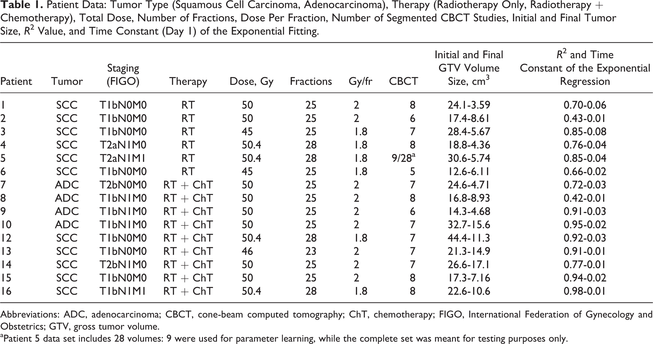
Abbreviations: ADC, adenocarcinoma; CBCT, cone-beam computed tomography; ChT, chemotherapy; FIGO, International Federation of Gynecology and Obstetrics; GTV, gross tumor volume.

^aPatient 5 data set includes 28 volumes: 9 were used for parameter learning, while the complete set was meant for testing purposes only.

Simulation CT (used for planning) and CBCT imaging, being the latter acquired for patient set-up correction at each treatment fraction, were processed to reconstruct tumor volumes. The tumor extents were evaluated at the time of treatment planning, according to the guidelines and were found in the range of about 3 to 4 cm (equivalent diameter) corresponding to a mean volume of 23.7 cm³ (range: 12.6-44.4 cm³). Up to 50.4 Gy were delivered to all 15 patients in approximately 25 fractions, along a period of 40 to 60 days (Table 1). As far as the CT imaging (voxel size: 0.93 mm × 0.93 mm × 3 mm) is concerned, the standard procedure involved the positioning of two 2-mm silver seeds, useful as fiducial markers, into the cervical tumor at the time of the simulation procedure.

Patients were scanned in supine position with a Combifix (CIVCO Medical Solutions, Kalona, Iowa) immobilization device, with a mean bladder volume of 400 cm³ (range 145-630 cm³). There was an interval of about 10 to 20 days from the CT acquisition to the beginning of treatment in order to elaborate the plan and pretreatment dosimetry. At each treatment fraction, patient set-up was verified by means of a kV CBCT system (voxel size: 0.87 mm × 0.87 mm × 3 mm) integrated in the treatment machine and corrections were performed according to the institutional (European Institute of Oncology, Milan, Italy) set-up verification and action level protocols. A subset of the acquired CBCT scans (Figure 1) was processed by an expert radiation oncologist through manual delineation, to extract the gross tumor volume (GTV).

Figure 1.

Patient 5: gross tumor volume (GTV; contoured) evolution outlined on cone-beam computed tomography (CBCT) images where t (days) is the time distance from the first radiotherapy fraction.

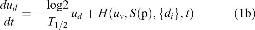
Tumors during radiotherapy consist of viable and dead cells, which have not been removed yet, characterized by 2 different dynamics.¹⁸ Viable cells (living clonogens) undergo a spontaneous growth that is counteracted by the cell-killing action due to radiation. As a consequence, the necrotic portion of the viable cells increases the population of dead cells, which are cleared, through a time-dependent mechanism (dead-cell resolving), from the tissue.^19,20 The variation over time t of the viable cell density u_v and the dead cell density u_d can be modeled in the following differential equation system as a function of the growth and the radiosensitivity parameter set (p), along with the fractionation schedule, as:

\frac{d u_{v}}{d t} = \frac{d G (u_{v}, t)}{d t} - H (u_{v}, S (p), \{d_{i}\}, t)

\frac{d u_{d}}{d t} = - \frac{log 2}{T_{1 / 2}} u_{d} + H (u_{v}, S (p), \{d_{i}\}, t)

where

u_{v} (t) + u_{d} (t)

represents the current overall number of tumor cells. In Equation 1a, the derivative of the proliferation function G contributes to increase the viable population, whereas the differential contribute H of the therapy induces a reduction of u_v. H depends on the cell density u_v, the survival fraction of viable cells S(p), and the fractionation regimen of the radiation therapy through the set of doses d_i (Gy). In the second equation, T_1/2 corresponds to the dead cell resolving half-time, which controls the exponential decay of the density u_d.

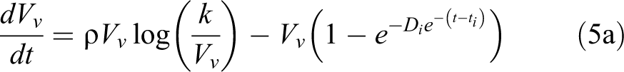
Uterine cervical tumors are typically solid and quite compact. Assuming the tumor is homogeneously irradiated and a linear radial evolution, the cell density can be thereby equivalently substituted with a tissue-scale geometric variable like the tumor volume.²¹ Taking into account the Gompertzian growth, the cell proliferation function G can be turned into Ğ representing the evolution in time of the viable volume V_v,

\overset{˘}{G} = V_{v} = k e^{(log (\frac{V_{v} (0)}{k}) e^{(- ρ t)})}

where ρ, k, and V_v(0) are the growth rate, the growth saturation factor of the volume (tissue capacity at cellular scale), and the volume at initial time, respectively. Equivalently, the cell density u_d in Equation 1b can replaced with the volume V_d. The GTV segmented on the images corresponds to the sum

(V = V_{v} + V_{d})

of the 2 volume contributes.

After a single radiation dose d_i, S_i is traditionally represented as a function of the parameters α (Gy⁻¹) and β (Gy⁻²) of the LQ model as:

S_{i} = e^{- (α d_{i} + β d_{i}^{2})}

Accounting for N radiation fractions, Equation 1a can be rewritten as:

\frac{d V_{v}}{d t} = ρ V_{v} log (\frac{k}{V_{v}}) - V_{v} \sum_{i}^{N} h (S_{i}, t)

where

h (S_{i}, t) = δ (t - t_{i}) (1 - e^{- (α d_{i} + β d_{i}^{2})})

represents the tumor cell mortality rate due to instantaneous (Dirac δ function) radiation effect at time t_i for the dose d_i. Fundamentally, the contribution of each dose fraction can be mathematically assumed equivalent to the δ function and appears as a signal term in the differential problem, which contributes to modulate tumor regression. The ordinary differential equation (ODE) system can be solved by subdividing the time interval into a series of N subintervals, such that δs always fall on the starting point of an interval. Given the instantaneous radiation effect at time t_i, the ODE is solved from the time t_i of i-th fraction to the time

t_{i + 1}

of the next fraction. Time

t_{i + 1}

is then used as the initial time for solving over the next subinterval. In fact, cell death due to irradiation occurs on a temporal window that is dependent upon many subject- and tumor-specific factors. It was shown that radiotherapy is not limited to direct DNA damage but encompasses several indirect complications at cell and tissue scales, ranging from indirect cellular apoptosis of nonirradiated cells²² and soft tissue fibrosis²³ to vascular damages with even major vessel rupture.²⁴ All these indirect effects of radiation are not instantaneous and can be delayed on short, mid, and even long temporal windows. A short-time effect was here considered by replacing in Equation 4 the differential component (δ function), corresponding to the radiation response, with an explicit exponential decay over time of the unitless effective dose

D_{i} = α d_{i} + β d_{i}^{2}

. This constitutes a technical novelty, with respect to prior similar modeling approaches^8,14 that in principle can allow dealing with nonuniform fractionation schedules. However, the introduction of this exponential term reduces the percentage of surviving cells per dose assuming the same tumor radiosensitivity

(α)

. Such occurrence should be taken into account in the result analysis since it is likely to lead to a slight underestimation of α with respect to the literature values. Considering 2 following irradiation time steps

\{t_{i}, t_{i + 1}\}

, the complete differential model can be then expressed as:

\frac{d V_{v}}{d t} = ρ V_{v} log (\frac{k}{V_{v}}) - V_{v} (1 - e^{- D_{i} e^{- (t - t_{i})}})

\frac{d V_{d}}{d t} = V_{v} (1 - e^{- D_{i} e^{- (t - t_{i})}}) - \frac{log 2}{T_{1 / 2}} V_{d}

The double exponential decay $(e^{- D_{i} e^{- (t - t_{i})}})$ makes the irradiation effects negligible (<10%) after 2 days considering average tumor and treatment features (α = 0.3 Gy⁻¹, d_i = 2 Gy). Therefore the summation introduced in Equation 4 was discarded in Equations 5a and 5b.

Four main modeling assumptions were hereafter detailed, regarding the relation between viable and dead-cell volumes, the parameter bounds used in the model learning, volume data normalization, and the nominal dose with respect to the effective dose delivered to the tumor. It was extensively reported that the therapeutic treatment of uterine cervical cancer through radiotherapy leads to a significant tumor regression on a daily basis, with significant volume shrinkage and even to a complete reabsorption.^8,25,26 Notably, Bondar et al.³ reported a mean tumor reduction of about 60% after 45 Gy. The tumor regression profiles in our study were mostly in agreement with such clinical observations as we measured an average daily shrinkage of about 5% per day in the first 5 treatment fractions and an overall tumor reduction of about 62% after about 45 Gy, on average. This evidence was the basis for arguing that such a fast tumor regression can be attributed to the quick dead-cell removal. Assuming that the necrotic volume is negligible with respect to the actual viable volume, during the treatment course, we can disregard from the model the dead-cell dynamics. In order to verify experimentally this simplification (V ∼ V_v), the complete model (cM) underwent the parameter learning on the GTV regression curve of patient 5 for whom we had all the segmentations along the entire treatment course. Nonetheless, from the mathematical point of view, the learning of the 4 parameters (ρ, k, α, and T_1/2) from the 2-equation differential system (5a) and (5b) with the constraint $(V = V_{v} + V_{d})$ is not a well-posed problem as the ratio $V_{d} / V_{v}$ is unknown. Setting T_1/2 to a discrete sample of values and performing for each value a dedicated learning of the other 3 parameters allows to improve the problem conditioning. Without lack of generality, the upper bound for T_1/2 was set to 30 days according to a previous report.⁸

In the model learning, the parameters were bounded by considering the initial volume values, the shape of the tumor regression curves, and the previous literature. As far as the volume carrying capacity k is concerned, given that no patients were surgically treated before radiotherapy, it was assumed that the initial volume was close to the maximum carrying capacity. This was confirmed by virtue of that the maximum volume increase over the first CBCT was about 15%, on average across patients. The setting of 50 < k (%) < 200 aimed at tolerating both a carrying capacity increase up to 100% and a decrease up to 50%.

The range of ρ was set between 0.01 and 1, which allowed the model to deal with both very slow (theoretically ∼600 days to achieve the nominal carrying capacity of 100%) and very fast growth rates (theoretically ∼10 days to achieve the nominal carrying capacity of 100%). Early data reported in the literature, about doubling time of the uterine cervical cancer (exponential growth), ranged from 3.1 to 5.6 days.²⁷ Although it is not straight-forward to correlate the growth rate of a Gompertzian function to the double-time of a simpler exponential growth, the ρ range was adequate to cope with such doubling time variability. The radiosensitivity parameter range (0 < α < 1 Gy⁻¹) was largely sufficient to include the various values reported in the literature.²⁸ The α/β ratio was setup to 10 Gy, taking into account the moderate rate of cell proliferation and well responsive tumors as in the case of uterine cervical cancer.²⁹ In fact, in the case of prostate cancer, which is a very slowly proliferating tumor, late responding tissue α/β can be as low as 1 Gy. At the other end of the range, α/β may be as high as 20 Gy in the case of advanced head and neck cancer, which is an early responding tissue with an extremely aggressive rate of cell proliferation. This operative choice was supported by the fact that most of the patients underwent a regular 5-day/wk treatment schedule. The volume V was normalized with respect to the first CBCT value as follows: $V (t) = 100 (V_{a b s} (t) / V_{a b s} (t = 0))$ , where $V_{a b s}$ is the absolute measured volume value. The normalization allowed us to compute averaged parameters able to fit the complete data cohort independently of the initial volume size. Finally, the nominal dose was assumed to be delivered homogeneously to the overall GTV volume, since the planning target volume (PTV) takes into account both invisible tumor lesion and possible organ shape deformations.

Two different variants of Equation 4 were considered in the learning phase, by assuming either a Gompertzian (6a) or a logistic growth curve (6b):

\frac{d V_{v}}{d t} = ρ V_{v} log (\frac{k}{V_{v}}) - V_{v} (1 - e^{- D_{i} e^{- (t - t_{i})}})

\frac{d V_{v}}{d t} = ρ V_{v} (1 - \frac{V_{v}}{k}) - V_{v} (1 - e^{- D_{i} e^{- (t - t_{i})}})

The single dynamic model was trained both on each patient individually (pM) and on the complete patient cohort (cM). The ODE resolution was performed by setting $V_{v} (t = 0)$ equal to the initial CBCT volume for each patient. In order to investigate the suitability of the general model (active and necrotic volumes), we tested it using the complete volume data set of patient 5 (Table 2).

Table 2.

Model Variants Considered in the Analysis.^a

Model	Training Set		Dynamic		Proliferation
Model	Single Patient	All Patients	V_v	$V_{v} + V_{d}$	Gompertzian	Logistic
cMg		×	×		×
cMl		×	×			×
pMg	×		×		×
pMl	×		×			×
gMg	×^a			×	×

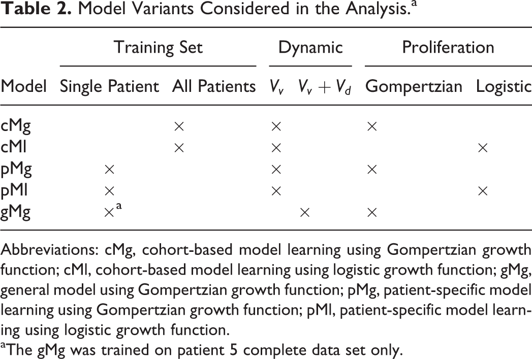
Abbreviations: cMg, cohort-based model learning using Gompertzian growth function; cMl, cohort-based model learning using logistic growth function; gMg, general model using Gompertzian growth function; pMg, patient-specific model learning using Gompertzian growth function; pMl, patient-specific model learning using logistic growth function.

^aThe gMg was trained on patient 5 complete data set only.

A custom genetic-based optimization procedure (Figure 2), implemented in Matlab (Matworks), was developed to train the models. Basically, a model parameter set (the proliferation rate ρ, the tumor cell carrying capacity k, and the radiation-specific parameter α) was iteratively estimated by exploiting competition in between a population of candidate parameter settings. The fitness measure was defined as follows: let $e_{i, j} = (V_{i, j} - {\overset{ˉ}{V}}_{i, j})$ be the difference between the predicted and measured tumor data for the j-th measurement of the i-th patient; being N_i the number of reconstructed tumor volumes for patient i and P the number of patients in the PS, the fitness E, associated to 1 parameter set, was calculated in terms of the root mean squared (RMS) error e_i, averaged across patients, as:

e_{i} = \sqrt{\frac{\sum_{j}^{N_{i}} e_{i, j}^{2}}{N_{i}}} E = \frac{1}{P} \sum_{i}^{P} P_{i}

At time instant t = 0, the algorithm started with the random generation of 150 different parameter sets in the population. For each parameter set, the differential Equation 4 was solved at each irradiation instant. When a measured tumor data

({\overset{ˉ}{V}}_{i, j})

was available, the corresponding

V_{i, j}

was computed and, by cumulating all the

e_{i, j}

, Equation 7 was used to determine the fitness for the current parameter set. According to the fitness results, a subset of the population was selected to be the candidate for reproduction through cross-over (recombination rate: 0.4) and mutation (mutation rate: 0.35) generating a new population at the next iteration step. The model training was iterated until the variance of the parameter set was lower than a threshold quantity ϵ (cfr Figure 2). In order to avoid premature convergence to local minima, the number of iterations was enforced to be greater than 200. The final model reliability was assessed in terms of fitting error E (Equation 7). Statistical comparison between patient subgroups (PSI, PSII, and PSIII) was performed upon parameter values (patient-specific model learning using Gompertzian growth function [pMg]) and fitting results (cM learning using Gompertzian growth function [cMg] and pMg) using the nonparametric Mann-Whitney test with a significance threshold P = .05.

Figure 2.

Chart of the genetic-based model parameter optimization.

In order to evaluate the extrapolation capabilities of the cM model, that is, its ability to predict tumor response and regrowth for a patient not included in the data set used for model learning, we implemented an approach based on the leave-one-out (LOO) technique. Without loss of generality, the prediction quality was assessed for cMg. The model was trained using the volume regression data of 14 patients while 1 patient data set was excluded. The relative extrapolation error for a given patient i was computed as:

{\overset{˘}{e}}_{i} = \sqrt{\frac{\sum_{j}^{N_{i}} {({\overset{˘}{V}}_{i, j} - {\overset{ˉ}{V}}_{i, j})}^{2}}{N_{i}}}

where

{\overset{˘}{V}}_{i, j}

is the volume predicted by the model. The extrapolation error, obtained by averaging the prediction errors over the patients in the data set, was compared to the fitting error computed from the model, which was trained over the whole patient data set.

In order to estimate pM extrapolation capability, the parameter set, computed on patient 5 (pMg5), was tested on: (1) patient 5 complete data set, (2) the other 5 patients belonging to PSI, and (3) patients in PSII and PSIII. The pMg2 was also tested on the 3 PS for comparison. The stability of the prediction outcomes in relation to small variations in the model parameter was also evaluated for the model cMg by means of a linear sensitivity analysis (LSA).

A different procedure was performed on cMg and pMg performed on the complete data set of patient 5 (pMg5*) to evaluate the effect of the data uncertainty on model parameters and prediction error consisting of 3 steps:

a Gaussian error (μ = 0, σ = 5) was added to the normalized volumes to simulate a 5% uncertainty of the volume measurements;

a new parameter set (ρ′, k′, and α′) was estimated using the perturbed data;

(ρ′, k′, and α′) were applied to the measured volumes and the error variation was computed.

Results

Parameter learning (ρ, k, and α) of the complete model, defined by Equations 5a and 5b, was performed on the overall volume data set (N = 28) of patient 5. The parameter T_1/2 was set to 5 constant values ranging from 0.5 to 30 days, and the learning was repeated for each of such values. Notably, the model ability to fit the volume data decreased significantly with the increase of T_1/2 (Figure 3), with errors ranging from about 8% $(T_{1 / 2} = 0.5)$ up to more than 40% ( $T_{1 / 2} = 30$ ; Table 3).

Figure 3.

Fitting error tendency for general model (gM) as a function of T_1/2.

Table 3.

The cMg Comprehensive Result Chart: T_1/2, Errors, and Parameter Values.

T_1/2, Days	E %	ρ	k	α
0.5	8.05	0.06	80.00	0.11
1	9.02	0.07	80.41	0.14
5	12.67	0.11	80.00	0.50
10	17.25	0.05	80.00	0.50
30	41.24	0.05	80.00	0.50

Abbreviation: cMg, cohort-based model learning using Gompertzian growth function.

Remarkably, the error trend at $T_{1 / 2} = 0.5$ was very close to the value achieved by means of pMg5* using the single dynamic approach (∼7%). In Figure 4, the predictions achieved with 2 different T_1/2 values were displayed for comparison. The necrotic volume percentage (on average) resulted about 6% of the total volume at $T_{1 / 2} = 0.5$ , whereas at $T_{1 / 2} = 10$ such quantity increased up to about 90%. Such results indicated that the model fitting quality was acceptable only with very small values of T_1/2 corresponding to a very fast dead-cell removal. Because of the general tumor shrinkage across the patient cohort, the model was simplified by taking into account the dynamics of the active volume only.

Figure 4.

Fitting results achieved using general model using Gompertzian growth function (gMg) are shown for $T_{1 / 2} = 0.5$ (A) and $T_{1 / 2} = 10$ (B). Diamond and squared marks represent the measured and predicted volumes, respectively. Necrotic (V_d) and viable (V_v) volume evolution are displayed in dashed and dash-dot lines, respectively. Circular dots at the baseline correspond to the irradiation days. Time t = 0 corresponds to the first radiotherapy fraction.

Despite their different formulation, the 2 models (cMg and cMl), trained on the whole patient cohort, showed similar performances (mean error: ∼16%), suggesting that Gompertzian and logistic functions are both able to mimic the tumor spontaneous growth dynamic (Table 4).

Table 4.

The cMg and cMl Performances and Optimal Parameters.

	cMg			cMl
E, %	Parameters			E, %	Parameters
	ρ	k	α		ρ	k	α
15.96	0.09	62.35	0.03	15.83	0.09	60.58	0.03

Abbreviations: cMg, cohort-based model learning using Gompertzian growth function; cMl, cohort-based model learning using logistic growth function.

As expected, the fitting performance of pM was better than that of the patient-cohort model (Table 5). Again, pMg and patient-specific model learning using logistic growth function (pMl) models were in good agreement with no significant difference (P > .1). The intergroup statistical analysis of the fitting errors did not provide significant differences (P > .1), using pMg and pMl as well. Therefore, it was not possible to assert any correlation among the model performances and the tumor histology or treatment. Wide-ranging variations in the parameters were, however, obtained across patients.

Table 5.

The pMg and pMl Performance and estimated parameters.

		pMg				pMl
	e_i	Parameters			e_i	Parameters
	e_i	ρ	k	α	e_i	ρ	k	α
Pz1	7.84	0.24	50.78	0.25	7.21	0.29	50.00	0.20
Pz2	5.02	1.00	61.76	0.13	4.72	1.00	58.23	0.06
Pz3	3.39	0.15	97.05	0.29	3.90	0.38	101.76	0.40
Pz4	5.78	0.17	97.64	0.26	5.01	0.09	87.05	0.05
Pz5	7.28	0.09	83.52	0.15	6.42	0.25	95.88	0.25
Pz6	6.84	0.13	104.11	0.12	6.35	0.12	101.76	0.09
Pz7	5.88	0.16	98.23	0.20	5.88	0.25	96.47	0.20
Pz8	6.47	0.29	87.05	0.11	6.53	0.33	87.05	0.11
Pz9	8.79	0.02	157.64	0.04	8.26	0.02	162.35	0.04
Pz10	3.24	0.06	78.82	0.04	4.08	0.11	98.23	0.06
Pz12	7.11	0.06	90.00	0.07	6.62	0.12	97.64	0.09
Pz13	4.89	0.13	102.94	0.04	5.95	0.25	104.11	0.06
Pz14	2.53	0.68	100.00	0.22	2.45	0.93	100.00	0.26
Pz15	7.53	0.02	117.05	0.03	7.23	0.02	124.70	0.03
Pz16	6.88	0.02	121.76	0.03	4.06	0.02	191.76	0.04
Mean (SD)	6.3 (1.82)	0.25 (0.27)	100.5 (25.1)	0.18 (0.09)	5.97 (1.56)	0.31 (0.30)	108.5 (35.2)	0.16 (0.11)

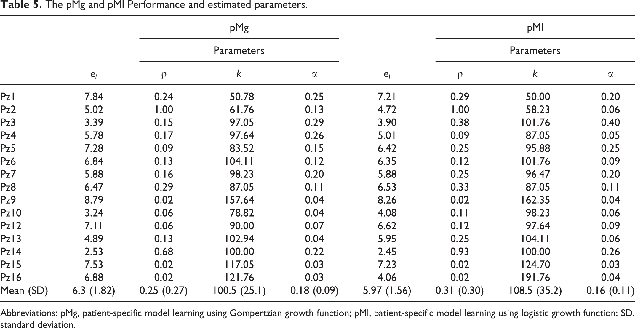
Abbreviations: pMg, patient-specific model learning using Gompertzian growth function; pMl, patient-specific model learning using logistic growth function; SD, standard deviation.

A few patients presented a peculiar tumor evolution with respect to the average exponential-like regression. For example, patient 2 who presents a different regression dynamic: after an initial significant shrinkage (Figure 5), the tumor reaches an almost constant size (∼50% of the initial volume). In such a patient, the carrying capacity was estimated to be significantly lower (k ∼62 and ∼58 for pMg and for pMl, respectively) than the others. This could be ascribed to an overcome of the sustainable size, the consequent lack of nutrients might have caused an accelerated (ρ = 1) reduction of the volume toward the carrying capacity value. Interestingly, the corresponding α value was quite small (0.13 for pMg and 0.06 for pMl): this could be due to a lack of adequate vascularization with consequent hypooxygenation and radiosensitivity reduction, in agreement to what suggested by the ρ and k results. The relative errors spanned across the range 2% to 10% both for pMg and pMl (Table 5). The highest error level was reported for patient 1, likely due to the sudden regrowth, at the beginning of the treatment (Figure 5, panel a), that the model was not able to reproduce. Patient 9 led to a k > 150 both for pMg and pMl; this might be due to its initial limited extent (about 14 cm³ corresponding to a 1.5 cm equivalent radius). Patients 16 (initial CT volume: 21 cm³) and 15 (initial CT volume: 19 cm³) resulted in great k values, as well. In contrast, patient 13 resulted in 100% < k < 105% despite its small initial size (13 cm³). The patients with the largest initial tumor sizes (patients 5, 10, and 12; V ∼ 50 cm³) resulted in 80% < k < 90%.

Figure 5.

Fitting results for patient-specific model learning using Gompertzian growth function (pMg) trained on patients 1 (A) and 2 (B). Diamond and squared marks represent the measured and predicted volumes, respectively. Circular dots at the baseline correspond to the irradiation days.

Significant intergroup statistical difference was found only for the α parameter. PSI turned out to be the most radiosensible patient set (mean α ∼ 0.2 Gy⁻¹) with a difference (P < .02) with respect to the other 2 patient sets. Interestingly, such a greater radiosensitivity was correlated only to the elderly patients in PSI while they underwent radiotherapy without adjuvant ChT.

Extrapolation results, obtained through the LOO technique, showed on average only a small increase of the prediction error with respect to the corresponding fitting error (Figure 6). As far as the pM is concerned, the parameter combination computed on the partial data set of the patient 5 (pMg5, E∼7%) was able to predict the complete tumor regression with a similar ability (E∼9%). pMg5 performance decreased in the attempt of predicting the other 5 patients belonging to PSI (E∼19%) as shown in Figure 7. However, the relative error value was comparable to the one achieved by cMg in the LOO procedure (cfr Figure 6). Finally, the performance achieved on PSII and PSII patients was unexpectedly even more promising (E∼16% on average). This restates that the patient subdivision into 3 PS was not meaningful, in agreement with the results of former statistical tests. pMg2 extrapolation ability was tested on the other 14 patients (excluding patient 2) as well, and a much higher mean prediction error was obtained (E∼26%).

Figure 6.

Leave-one-out (LOO) results obtained training cohort-based model learning using Gompertzian growth function (cMg) on 14 patients at a time and testing the parameter combination on the left-out-patient. The training and testing errors are showed for each patient (left panel) and on average taking into account the standard deviation (right panel).

Figure 7.

Extrapolation results obtained by pMg performed on the reduced data set of patient 5 (pMg5) on another patient of PSI (patient 6). Diamond and squared marks represent the measured and predicted volumes, respectively. Circular dots at the baseline correspond to the irradiation days.

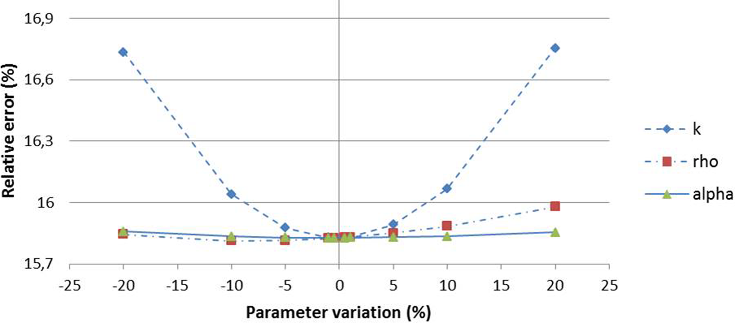
Considering the cohort-based model (cMg), a perturbation in α and ρ values up to 20% produced a very small error increase, namely $|E (ρ, k, α^{'}) - E (ρ, k, α)| < 0.2 %$ and $|E (ρ^{'}, k, α) - E (ρ, k, α)| < 0.03 %$ , respectively. The effect of k variation, although more relevant, reflected in a maximum error increase of about 1% (Figure 8), indicating that the model is more sensitive to k value.

Figure 8.

The LSA results for cohort-based model learning using Gompertzian growth function (cMg). Dashed, continuous, and dot-dashed lines represent the sensitivity curves of ρ, k, and α, respectively.

cMg(Ṽ) and pMg5*(Ṽ) were trained on the related noisy volumes $Ṽ = V + N (0.0, 5.0)$ data sets. $Ṽ$ was affected by an average 5% uncertainty level computed as $(Ṽ (t) - V (t)) / V (t = 0)$ with respect to the average initial volume (about 1.5 cm³). If we assume a tumor spheroid shape, this value implies about 0.1 mm error on the equivalent diameter of a 30-cm³ tumor and up to 2 mm on a 6.3-cm³ volume (corresponding to the initial and final patient 5 tumor sizes, respectively) and to an average value of the error $e p s = (Ṽ (t) - V (t)) / V (t)$ close to 20%. The resulting k and α variations were lower than 5% for both cMg and pMg5*, whereas ρ decreased of about 8% for pMg5* and increased of about 30% for cMg. This last variation, however, was very small when compared to the mean absolute value (0.09) of ρ. The corresponding difference of the fitting errors was lower than 0.1% and 0.2% for cMg and pMg5*, respectively.

Discussion

The models proposed in this work achieved promising fitting performances (E∼16% and E∼6% for cM and pM, respectively). Comparable results were obtained by means of the Gompertzian and logistic proliferation models. cMg prediction ability, assessed by means of the LOO procedure, was only slightly lower (E∼18%) than the original fitting performance (E∼16%). As expected, the pMg learning approach was able to better fit each specific patient volume regression. Interestingly, pMg5 also showed an extrapolation ability comparable to cMg (19% and 16% on PSI and PSII + PSIII, respectively). However, patient 5, whose reduced data set was exploited to train pMg5, showed a rather exponential-like regression (R² = .85, crf. Table 1). The model trained on patient 2 data set (R² = .43) led to significantly different results (E∼26%) in predicting the tumor regression of the other patients. No significant differences were found across the 3 PS in terms of fitting errors. The parameters, optimized on each single patient (pM), were not statistically different with respect to the tumor histology and delivered treatment. The only exception was represented by the radiosensitivity parameter in PSII and PSIII, which was lower on average with respect to that of PSI (P < .02). This is apparently in contrast with the fact that chemoagents were administered to both PSII and PSIII, but in agreement with the measured regression rates (cfr Table 1, last column).

Notably, the model was shown to be robust to both parameter and volume data perturbation. In particular, we found a very small fitting error increase (0.2%) with respect to a simulated tumor volume size variation of about 20%, making the model suitable to be applied on noisy CBCT data.

Tumor growth and therapy response were represented by using continuous equations (ODE) and limiting the model description to the tissue level and macro-scale growth mechanisms. Mathematically more sophisticated generalizations of various kinds (eg, multiple cell status to discriminate between necrotic and hypoxic tumor fraction, effect of vascularized tumors) can enhance the realism of the model. Nonetheless, the corresponding increase in the parameter number and the difficulty of constraining them, using imaging data, makes more complex models less practical for clinical use.

The underlying assumption of a fast dead-cell dynamic, allowing the use of the single-dynamic model, was mostly supported by the major tumor shrinkage we measured on a daily basis. The applicability of the single-dynamic model to different fitting or prediction problems should always be verified on the specific data set under analysis. Although the double-dynamic is biologically more consistent than the single dynamics, the parameter learning problem is not well-posed. Without properly conditioning the $V_{d} / V_{v}$ ratio, the relation $v = V_{v} + V_{d}$ is insufficient to constraint the resolution of the ODE system, leading to uncertainty of the solution for the parameters (ρ, k, α, and T_1/2). Gathering functional and histological information along the course of treatment would be the practical approach to address the question, while its feasibility is still a critical aspect in IGRT (eg, cost, invasiveness, and time). Perspective studies could be considered, for example, exploiting positron emission tomography functional images capturing tumor activity or, in the particular case of cervix cancer, assessing the tumor perfusion by means of Doppler sonography.^30,31

The volume normalization allowed us to apply the same model to all the patients (cMg/cMl) computing a unique sensitivity parameter α independently on the initial tumor size. However, α (as well as ρ, k) is likely to vary significantly on a patient-specific basis since the active layer is composed by several cell lines featuring different radiosensitivity.³² The solid and compact nature of cervical cancer may also cause the onset of hypoxic regions. It was extensively reported that the oxygen distribution in a tumor has a significant effect on radioresponsivity and prognosis.^31,33,34 Some works addressed the problem by modeling spheroids featuring multiple necrotic cores.³⁵ Another possible approach is to include further information on the well-known hypoxic fraction (HF) which could be estimated noninvasively by means of magnetic resonance imaging (MRI) acquisitions³⁶ and to relate it to the oxygen enhancement ratio (OER) accounting for the increased effectiveness of the radiation in presence of higher oxygen concentration. Moreover, the tumor features evolve during the treatment period, for example as a consequence of vascular modifications.³⁷ The α parameter assessed by our simplified model corresponds to an average value across the overall treatment period. The modeling of the radiosensitivity dependency upon hypoxia was beyond the purpose of the present study, however it could be introduced by considering $α (p O_{2} (t))$ , where $p O_{2} (t)$ represents the oxygenation level trough time.

Two main sources of uncertainty should be considered in this work, namely the tumor delineation errors in the CBCT images and the difference between the nominal and the real doses delivered to the patient. We acknowledge that CBCT is a suboptimal imaging modality, but a systematic analysis of the quantification of the CBCT tumor delineation variability was out of the scope of this article. Tumor volume was manually delineated on the simulation (planning) CT and then on every CBCT by the same operator. Inter- and intraobserver variability is a well known pitfall in modern radiotherapy of numerous tumors³⁸ and regards all procedures like diagnostic imaging, target contouring, and image-based target verification during treatment course. Indeed, CBCT image interpretation represents an issue for CBCT-based IGRT. When compared to other imaging modalities, such as CT or MRI, CBCT carries the highest interobserver variability in target and organs at risk identification. These difficulties are due to the lack of contrast medium and reduced image quality. Segmentation and delineation assessment, as well as the analysis of interobserver variability are part of the IGRT quality assurance program.³⁹ In one study,⁴⁰ the authors reported an interobserver variability for prostate delineation on CBCT images lower than 2 mm. In another study,⁴¹ the authors reported a similar interobserver variability (∼1 mm) for bladder delineation on CBCT images. Recently, guidelines for reporting contouring variability have been proposed.⁴² In the present article, we performed a test to evaluate the model robustness by simulating data uncertainty. Considering a reasonable uncertainty of 5% of the measured volumes, with respect to the initial tumor size, we remarkably obtained a fitting error variation lower than 0.2%.

The nominal value of the dose delivered to the patient was used despite the possible occurrence of errors due to tumor shape modification, soft tissue deformation and physical interaction with the surrounding organs. However, as the radiation is delivered according to the PTV, which is enlarged with respect to the GTV, the morphological deviations to planning are addressed, however at the cost of an increase in toxicity. In order to quantify the exact dose to the tumor, the image registration between CBCT and planning CT appears to be mandatory.

The reported results are promising, as they prove that concurrent proliferative regrowth and radiation cell killing effects are sufficient to represent tumor regression in cervical cancer. The applied models did not make any assumption about radiotherapy or ChT killing mechanisms at a cellular level, as only cell survival fractions were used. Therefore, these equations can be applied to radiotherapy or combined radiotherapy and ChT treatments, in temporally nonuniform treatment scheduling. In conclusion, the main contributions of this study can be summarized as follows: (1) macroscopic proliferative and LQ radiosensitivity models can represent cervical cancer tumor regression within experimental uncertainties; (2) the difference between Gompertzian and logistic growth models is negligible; (3) tumor regrowth and radiobiological parameters can be evaluated both on patient- and group-specific basis. Potentially, the predictive ability of the model can be exploited to simulate how changes in the treatment schedule (number of fractions, doses, and intervals among fractions) can affect the tumor regression on an individual basis. One of the simplest appealing scenarios, disclosed by the use of such predictive models, would provide meaningful information to the physician at the time of treatment planning and during therapy administration, so that the therapeutic schedule can be adapted at run time accounting for patient specific tumor regression patterns observed on image guidance data.

Conclusions

In this study, we analyzed the potential ability of macroscopic time-continuous models to represent tumor response when trained on a patient-set and patient-specific basis. The ODE models, which integrate proliferative functions (Gompertzian and logistic) with the radiobiological LQ model, were implemented to cope with 2 concurrent tumor features, namely repopulation and sensitivity to radiation. The basic assumptions of the reported modeling effort were the following: (1) the tumor mass is characterized by a single cell type; (2) the regression is independent of the initial absolute tumor size; and (3) the radiation response is locally time-delayed and globally dependent upon the specific treatment schedule.

Serial CBCT data showed a general tumor regression in all of the 15 patients, in agreement with other studies, which observed tumor shape regression performed through megavoltage CT imaging.⁴³ These data (GTV volume) were used to learn model parameters by means of evolutionary optimization, accounting for 2 different histological cervical cancer types and different treatment regimens (with and without concomitant ChT). A short-time window (∼60 days), coincident with the irradiation period, was considered, and no follow-up measurements were taken into account.

Footnotes

Abbreviations

Declaration of Conflicting Interests

The author(s) declared no potential conflicts of interest with respect to the research, authorship, and/or publication of this article.

Funding

The author(s) received no financial support for the research, authorship, and/or publication of this article.

References

Sadozye

Reed

. A review of recent developments in image-guided radiation therapy in cervix cancer. Curr Oncol Rep. 2012;14(6):519–526. doi: 10.1007/s11912-012-0275-3.

Lindegaard

Fokdal

Nielsen

Juul-Christensen

Tanderup

. MRI-guided adaptive radiotherapy in locally advanced cervical cancer from a Nordic perspective. Acta Oncol. 2013;52(7):1510–1519. doi: 10.3109/0284186X.2013.818253.

Bondar

Hoogeman

Mens

. Individualized non-adaptive and online-adaptive intensity-modulated radiotherapy treatment strategies for cervical cancer patients based on pretreatment acquired variable bladder filling computed tomography scans. Int J Radiat Oncol Biol Phys. 2012;83(5):1617–1623. doi: 10.1016/j.ijrobp.2011.10.011.

Hoogeman

Quint

Bondar

Mens

Dhawtal

Heijmen

. OC-0147 Clinical implementation of the plan-of-the-day concept for IMRT of cervical cancer. Radiother Oncol. 2012;103(S1):S57. doi:10.1016/S0167-8140(12)70486-3.

Jadon

Pembroke

Hanna

. Systematic review of organ motion and image-guided strategies in external beam radiotherapy for cervical cancer. Clin Oncol (R Coll Radiol). 2014;26(4):185–196. doi: 10.1016/j.clon.2013.11.031.

Dionysiou

Stamatakos

Uzunoglu

Nikita

Marioli

. A four-dimensional simulation model of tumour response to radiotherapy in vivo: parametric validation considering radiosensitivity, genetic profile and fractionation. J Theor Biol. 2004;230(1):1–20. doi: 10.1016/j.jtbi.2004.03.024.

Sanga

Frieboes

Zheng

Gatenby

Bearer

Cristini

. Predictive oncology: a review of multidisciplinary, multiscale in silico modeling linking phenotype, morphology and growth. Neuroimage. 2007;37(suppl 1):20–34. doi: 10.1016/j.neuroimage.2007.05.043.

Huang

Mayr

Yuh

. Predicting outcomes in cervical cancer: a kinetic model of tumor regression during radiation therapy. Cancer Res. 2010;70(2):463–470. doi: 10.1158/0008-5472.CAN-09-2501.

Frieboes

Chaplain

Thompson

Bearer

Lowengrub

Cristini

. Physical oncology: a bench-to-bedside quantitative and predictive approach. Cancer Res. 2011;71(2):298–302. doi: 10.1158/0008-5472.CAN-10-2676.

10.

Jiao

Torquato

. Emergent behaviors from a cellular automaton model for invasive tumor growth in heterogeneous microenvironments. PLoS Comput Biol. 2011;7(12):1–14. doi: 10.1371/journal.pcbi.1002314.g009.

11.

Bankhead

III Heckendorn

. Using evolvable genetic cellular automata to model breast cancer. Genet Program Evol M. 2007;8(4):381–393. doi:10.1007/s10710-007-9042-x.

12.

Harting

Peschke

Karger

. Computer simulation of tumour control probabilities after irradiation for varying intrinsic radio-sensitivity using a single cell based model. Acta Oncol. 2010;49(8):1354–1362. doi: 10.3109/0284186X.2010.485208.

13.

Edelman

Eddy

Price

. In silico models of cancer. Wiley Interdiscip Rev Syst Biol Med. 2010;2(4):438–459. doi: 10.1002/wsbm.75.

14.

Rockne

Rockhill

Mrugala

. Predicting the efficacy of radiotherapy in individual glioblastoma patients in vivo: a mathematical modeling approach. Phys Med Biol. 2010;55(12):3271–3285.

15.

O’Donogue

. The response of tumours with Gompertzian growth characteristics to fractionated radiotherapy. Int J Radiat Biol. 1997;72(3):325–339. doi: 10.1080/095530097143329.

16.

Albano

Giorno

Román-Román

Torres-Ruiz

. Inferring the effect of therapy on tumors showing stochastic Gompertzian growth. J Theor Biol. 2011;276(1):67–77. doi:10.1016/j.jtbi.2011.01.040.

17.

Piotrowska

Foryś

Bodnar

Poleszczuk

. A simple model of carcinogenic mutations with time delay and diffusion. Math Biosci Eng. 2013;10(3):861–872. doi: 10.3934/mbe.2013.10.861.

18.

Okumura

Ueda

Mori

Kitabatake

. Kinetic analysis of tumor regression during the course of radiotherapy. Strahlentherapie. 1977;153(1):35–39.

19.

Brown

Attardi

. The role of apoptosis in cancer development and treatment response. Nat Rev Cancer. 2005;5(3):231–237. doi: 10.1038/nrc1560.

20.

Chvetsov

Palta

Nagata

. Time-dependent cell disintegration kinetics in lung tumors after irradiation. Phys Med Biol. 2008;53(9):2413–2423. doi:10.1088/0031-9155/53/9/013.

21.

Bentzen

Thames

. Tumor volume and local control probability: clinical data and radiobiological interpretations. Int J Radiat Oncol Biol Phys. 1996;36(1):247–251. doi: 10.1016/S0360-3016(96)00242-8.

22.

Prise

Schettino

Folkard

Held

. New insights on cell death from radiation exposure. Lancet Oncol. 2005;6(7):520–528. doi: 10.1016/S1470-2045(05)70246-1.

23.

Dormand

Banwell

Goodacre

. Radiotherapy and wound healing. Int Wound J. 2005;2(2) 112–127. doi: 10.1111/j.1742-4801.2005.00079.x.

24.

Davidson

Faithfull

. Late radiotherapy effects: is bowel morbidity adequately documented or patients’ needs managed appropriately? Clin Oncol. 2006;18(5):419–420. doi: 10.1016/j.clon.2006.03.005.

25.

Lim

Chan

Dinniwell

. Cervical cancer regression measured using weekly magnetic resonance imaging during fractionated radiotherapy: radiobiologic modeling and correlation with tumor hypoxia. Int J Radiat Oncol Biol Phys. 2008;70(1):126–133. doi:10.1016/j.ijrobp.2007.06.033.

26.

Schmid

Mansmann

Federico

. Residual tumour volumes and grey zones after external beam radiotherapy (with or without chemotherapy) in cervical cancer patients. Strahlentherapie und Onkologie. 2013;189(3):238–245. doi:10.1007/s00066-012-0260-7.

27.

Hill

Fyles

Milosevic

Pintilie

Tsang

. Is there a relationship between repopulation and hypoxia/reoxygenation? Results from human carcinoma of the cervix. Int J Radiat Biol. 2003;79(7):487–494. doi: 10.1080/0955300031000102641.

28.

Plataniotis

Dale

. Use of concept of chemotherapy-equivalent biologically effective dose to provide quantitative evaluation of contribution of chemotherapy to local tumor control in chemoradiotherapy cervical cancer trials. J Radiat Oncol Biol Phys. 2008;72(5):1538–1543. doi: 10.1016/j.ijrobp.2008.06.1911.

29.

Levine

Renehan

Gossiel

. Apoptosis, intrinsic radiosensitivity and prediction of radiotherapy response in cervical carcinoma. Radiother Oncol. 1995;37(1):1–9. doi: 10.1016/0167-8140(95)01622-N.

30.

Pairleitner

Steiner

Hasenoehrl

Staudach

. Three-dimensional power Doppler sonography: imaging and quantifying blood flow and vascularization. Ultrasound Obstet Gynecol. 1999;14(2):139–143. doi: 10.1046/j.1469-0705.1999.14020139.x.

31.

Redondo

Oresanz

Salazar

. The role of 3D ultrasound and 3D power. Doppler imaging in the diagnosis and. Evaluation of ovarian cancer: new perspectives. Donald School J Ultrasound Obstet Gynecol. 2007;1(2):38–41.

32.

Kelland

Steel

. Differences in radiation response among human cervix carcinoma cell lines. Radiother Oncol. 1988;13(3):225–232. doi: 10.1016/0167-8140(88)90059-X.

33.

Gray

Conger

Ebert

Hornsey

Scott

. The concentration of oxygen dissolved in tissues at the time of irradiation as a factor in radiotherapy. Br J Radiol. 1953;26(312):638–648. doi:10.1259/0007-1285-26-312-638.

34.

Hall

Giaccia

AJ.

Radiobiology for the Radiologist. Philadelphia, PA: Lippincott Williams & Wilkins; 2006. doi:10.1017/S1460396906000343.

35.

Grimes

Kelly

Bloch

Partridge

. A method for estimating the oxygen consumption rate in multicellular tumour spheroids. J R Soc Interface. 2014;11(92):20131 124. doi:10.1098/rsif.2013.1124.

36.

Zhang

Hallac

Peschke

Mason

. A noninvasive tumor oxygenation imaging strategy using magnetic resonance imaging of endogenous blood and tissue water. Magn Reson Med. 2014;71(2):561–569. doi:10.1002/mrm.24691.

37.

Cooper

West

CML

Wilks

. Tumour vascularity is a significant prognostic factor for cervix carcinoma treated with radiotherapy: independence from tumour radiosensitivity. Br J Cancer. 1999;81(2);354–358. doi:10.1038/sj.bjc.6690700.

38.

Jameson

Holloway

Vial

Vinod

Metcalfe

. A review of methods of analysis in contouring studies for radiation oncology. J Med Imaging Radiat Oncol. 2010;54(5):401–410. doi: 10.1111/j.1754-9485.2010.02192.x.

39.

Korreman

Rasch

McNair

. The European Society of Therapeutic Radiology and Oncology-European Institute of Radiotherapy (ESTRO-EIR) report on 3D CT-based in-room image guidance systems: a practical and technical review and guide. Radiother Oncol. 2010;94(2):129–144. doi: 10.1016/j.radonc.2010.01.004.

40.

Lütgendorf-Caucig

Fotina

Stock

Pötter

Goldner

Georg

. Feasibility of CBCT-based target and normal structure delineation in prostate cancer radiotherapy: multi-observer and image multi-modality study. Rad Oncol. 2011;98(2):154–161. doi: 10.1016/j.radonc.2010.11.016.

41.

Nishioka

Shimizu

Kinoshita

. Evaluation of inter-observer variability of bladder boundary delineation on cone-beam CT. Radiat Oncol. 2013;8:185–191. doi: 10.1186/1748-717X-8-185.

42.

Fotina

Lütgendorf-Caucig

Stock

Pötter

Georg

. Critical discussion of evaluation parameters for inter-observer variability in target definition for radiation therapy. Strahlenther Onkol. 2012;188(2):160–167. doi: 10.1007/s00066-011-0027-6.

43.

Kupelian

Ramsey

Meeks

. Serial megavoltage CT imaging during external beam radiotherapy for non-small-cell cancer: observations on tumor regression during treatment. Int J Radiat Oncol Biol Phys. 2005;63(4):1024–1028. doi:10.1016/j.ijrobp.2005.04.046.

Kinetic Models for Predicting Cervical Cancer Response to Radiation Therapy on Individual Basis Using Tumor Regression Measured In Vivo With Volumetric Imaging

Abstract

Keywords

Introduction

Materials and Methods

Results

Discussion

Conclusions

Footnotes

Abbreviations

Declaration of Conflicting Interests

Funding

References