Feasibility of Radiotherapy Fiducial Marker Tracking via Single-Shot X-ray Acoustic Tomography

Abstract

Introduction

in radiotherapy, fiducial markers improve the accuracy of radiation delivery, and their use has become increasingly important in the treatment of various cancers, particularly those in the prostate and lung. This work aims to determine, via Monte Carlo simulations and numerical ultrasound transport, the feasibility of fiducial marker localization via single-shot x-ray acoustic computed tomography.

Methods

patient data from CT scans for two treatment sites, prostate and lung, were used to model the fiducial marker localization process. Monte Carlo simulation was used to calculate the absorbed dose distribution in each patient resulting from the irradiation with a 120 kVp x-ray imaging source, assuming that the dose is imparted in a short pulse. Ultrasound transport through each patient was modeled with the numerical ultrasound transport package k-Wave. For the image reconstruction process, as the exact internal patient structure will not be known at the time of treatment, a homogenous medium with the patient external contour and dimensions was used.

Results

It is shown that the use of a homogeneous model to approximate the actual patient material composition during the reconstruction process, necessary as the geometry of the internal structures is not known at the time of the treatment, severely degrades the quality of the x-ray acoustic tomography images, but that it is still possible to determine the fiducial marker position with an accuracy of or better than 1 mm. The largest errors are observed for the lung patient when the lung is in an inflated state.

Conclusions

it has been shown that single-shot x-ray acoustic tomography can be an effective tool for the tracking and localization of radiotherapy fiducial markers, exhibiting an accuracy of better than 1 mm, despite the poor visual quality of the resultant images.

Introduction

Fiducial markers (FM), made of materials like gold, platinum, or carbon, are small objects implanted into or near a tumor to enhance the precision of radiotherapy treatments. These markers, typically inserted via minimally invasive procedures such as endoscopy, bronchoscopy, or percutaneous needle placement, serve as reference points within the body, allowing clinicians to accurately identify the location of a tumor during a radiotherapy treatment, despite patient movement or anatomical changes.^1,2 By providing a consistent and visible reference point, FM help align the radiation beams with the tumor more precisely, minimizing radiation exposure to surrounding healthy tissues. This precision is crucial in stereotactic body radiotherapy (SBRT) and intensity-modulated radiotherapy (IMRT), which involve delivering high doses of radiation to a targeted area while sparing adjacent structures. The markers also enable adaptive radiotherapy, where treatment plans are adjusted in real-time based on tumor movement or changes in size, enhancing overall treatment effectiveness. For this technique to be effective, a method to localize the fiducial markers in real time during the application of the radiotherapy treatment must be in place. The localization of the FM is usually carried out using diagnostic x-ray beams, with two systems currently in clinical practice: two ceiling mounted x-ray tubes with floor-mounted imaging sensors; and gantry mounted x-ray tube and imaging sensor. To obtain the spatial coordinates of each marker, two x-ray projections are needed, which is straightforward for the former system but that requires gantry motions to position the x-ray tube and imaging sensor at two different angles for the latter, thus interfering with the treatment flow. Several methods have been proposed to derive the FM positions from a single x-ray image, including the use of the radiation scattered by the FM to form the second image, ³ simultaneous kV and MV image acquisition in dual image systems, ⁴ or the use of the single x-ray image with an estimation of the target trajectory based on previously determined probabilistic distributions.^5,6,7

x-ray Acoustic Tomography (XACT) is an advanced imaging technique that integrates the strengths of both x-ray and acoustic imaging modalities to achieve high-resolution 3D visualization of internal structures in objects. The basic working principle of XACT involves exposing an object to pulsed x-rays, with pulse lengths in the order of nanoseconds: as x-rays are absorbed by different tissues or materials, localized heating occurs, leading to thermal expansion and contraction with the subsequent emission of ultrasonic pressure waves. ⁸ These acoustic signals are detected by a set of sensors placed on or very close to the object and reconstruction algorithms are then used to obtain the spatial distribution of the initial pressure wave, which is proportional to the x-ray absorbed dose imparted to the irradiated volume. ⁹ Among the several biomedical applications of XACT, breast imaging ¹⁰ and dosimetry verification of radiotherapy treatments^11,12 are actively being explored by several groups with promising results.

Unlike x-ray computed tomography, XACT can produce a full 3D image of an object with a single x-ray pulsed irradiation and a single planar ultrasound (US) sensor. This makes this imaging modality particularly well suited for the solution of several problems that arise in image guided radiotherapy, including fiducial marker tracking or seed and applicator localization in brachytherapy, as the burden of taking at least two x-ray projections, a process that may interfere with the treatment flow, is reduced. This has already been recognized before, and it has been shown that it is in principle possible to reconstruct gold FM with a resolution of 350 µm. ¹³ One caveat of this and other studies, is that the XACT images were obtained for homogenous media with smooth planar surfaces. In an actual patient, bone and pockets of air can severely distort the resultant XACT images. Furthermore, most XACT reconstruction algorithms assume a homogenous acoustic media and, therefore, it is necessary to evaluate if, when considering the complex material composition and geometry of a real patient, it is even possible to obtain the position of the FM with the better than 1 mm accuracy that it is possible using conventional x-ray 2D projections. This latter aspect is crucial in FM tracking: it is not enough to be able to visualize a set of markers, we also need to establish their position in a frame of reference that contains both the patient and the treatment machine. Otherwise, the reconstructed XACT images, regardless of their quality, are useless.

In this work, using Monte Carlo simulation and realistic patient data derived from CT images, we model the use of XACT as a FM 3D localization tool, from the dose deposition process to the reconstruction of the initial acoustic pressure that gives rise to the detected ultrasound signal. It will be shown that it is in principle feasible to use XACT for the FM tracking problem obtaining accuracies close to those obtained when using conventional x-ray radiographs, with the advantage that only one x-ray irradiation is needed, but that the resultant images lack the geometric sharpness characteristics of other 3D imaging modalities, such as CT and MRI.

Materials and Methods

Patient and Fiducial Marker Models

Two patient models derived from CT data are used in this work. The first model, representing a prostate cancer patient was taken from the segmented Zubal phantom at the pelvis level. ¹⁴ The resolution of this phantom is 0.4 × 0.4 × 0.4 cm³ and nine different materials were explicitly modeled using material composition taken from ICRU Report 44, ¹⁵ including compact bone, skeletal muscle, soft tissue, skin, with water used to model urine and feces. The second model represents a lung cancer patient with a tumor located in the periphery of one lung. This model was obtained from the Cancer Imaging Archive ¹⁶ and a calibration curve was used to convert the Hounsfield number to material composition and density, ¹⁷ with a total of 17 different materials modeled. The resolution of this patient model was 0.3 × 0.1 × 0.1 cm³. To increase the resolution of the dose calculation process, both phantoms were up sampled to a voxel resolution of 0.1 × 0.1 × 0.1 cm³.

The fiducial markers are assumed to be made of gold. While it is recognized that markers of different shapes and sizes are available, it was decided that the ability to fully embed the marker in the voxelized geometry would be necessary, as the software used to model the US transport, to be described below, necessitates a single 3D matrix of initial acoustic pressure values, obtained from the absorbed dose distribution. Therefore, the FM models in this work are rectangular cylinders with dimensions of 1 mm×1 mm×5 mm, consistent with the geometric features of several commercially available markers. Three such markers were digitally added to each of the patient models just described in different orientations. In the prostate patient in particular, the markers were placed in what may not be a realistic clinical configuration, with markers mutually perpendicular to each other. This was done with the express purpose of producing different absorbed dose distributions within the markers, as the initial US pressure amplitude directly depends on local dose. For the case when the marker axis runs parallel to the incident x-ray beam, the dose in the distal end would be severely attenuated by the 5 mm of gold, thus posing a challenge to the accuracy of the reconstruction.

Monte Carlo Simulation of the Initial Dose Deposition

The PENELOPE Monte Carlo radiation transport code ¹⁸ with the steering main program from the penEasy suite ¹⁹ were used to first calculate the absorbed dose distribution in each patient model produced by a diagnostic x-ray beam such as those used in linac on-board imaging systems, with a 120 kVp x-ray spectrum taken from the literature. ²⁰ Both photon and electron cutoff energies were set at 10 keV and, per the code developers, transport parameters C1 and C2 were both set at a value of 0.1. Standard PENELOPE package cross-sections files were used in all the simulations here presented. Figure 1 shows the irradiation geometry which was the same for both patient models. A sensor plane containing a plurality of individual US sensors, is placed at the shortest possible distance from the target and in such a way that thick bone structures are avoided. A single sensing plane is used to avoid interfering with the x-ray beam on its way to the patient. An x-ray image sensor was placed to obtain a radiograph from each phantom, with the purpose of comparing the 3D marker position obtained from XACT with their 2D projection on this lateral radiograph. The frame of reference used follows the PENELOPE convention in which the box enveloping the voxelized patient geometry is placed with one of its corners at the origin and within the first octant. Notice that the irradiation is carried out laterally in both cases, which may not be optimal, particularly for the prostate patient as the x-ray beam passes through the femoral heads, but this was done to avoid the direct x-ray irradiation of the space occupied by the US sensor. The PENELOPE dose matrices were normalized so that the average dose in the patient, excluding the gold markers, was 1 mGy. It is assumed that this dose is delivered in a pulse short enough to give raise to the photoacoustic effect, which is in the order of 50 ns. ²¹ Battery-powered kilovoltage x-ray tubes with the capability to achieve such short pulses are commercially available. ²² No attempt was made to model XACT FM localization with the high-energy radiotherapy beam as current linac technology lacks the capability of producing nano-seconds x-ray pulses.

Figure 1.

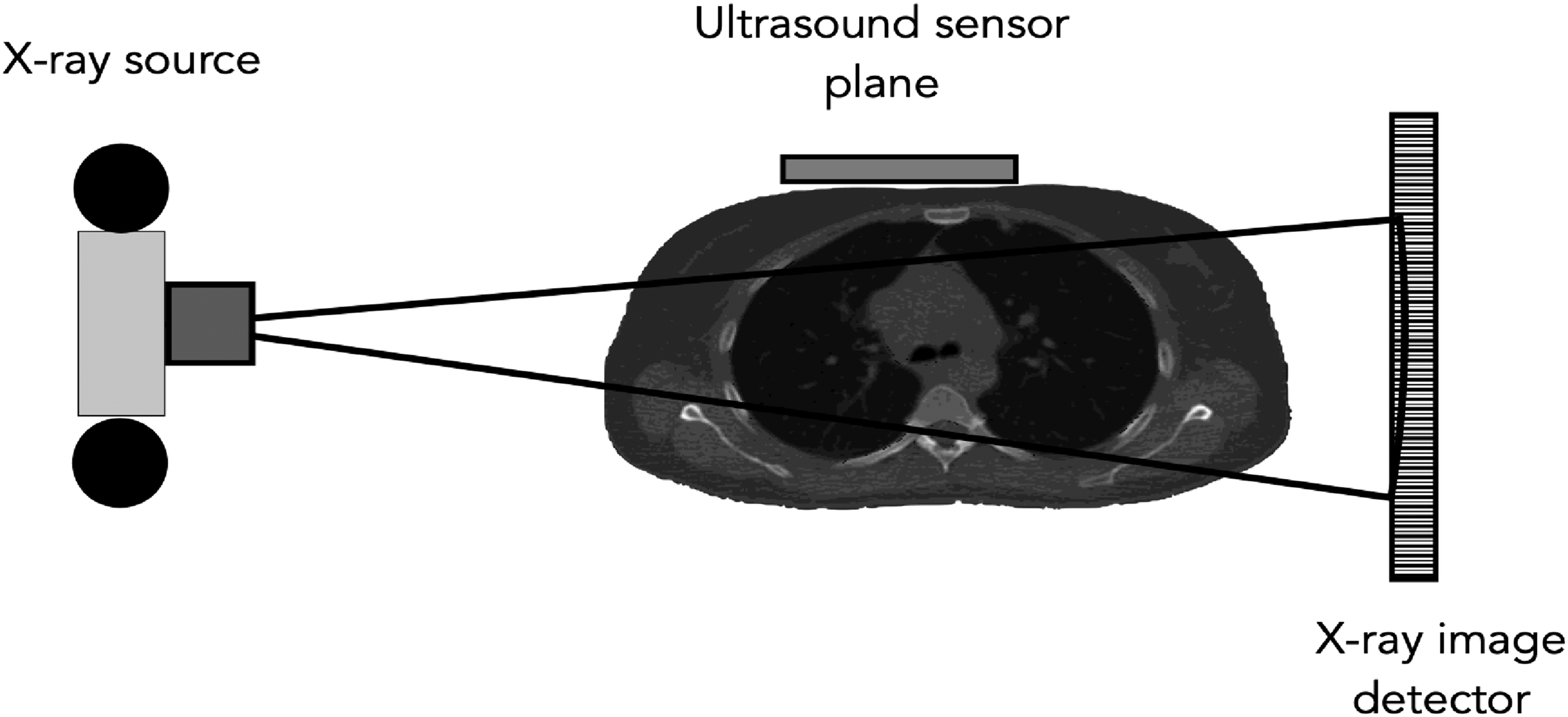
Irradiation Setup for Both Patient Models. The Ultrasound Sensor Array is Placed on the Anterior Side of the Patient and is Not Directly Irradiated by the x-Ray Beam.

Ultrasound Wave Propagation and Detection

The two patient phantom models and their respective dose matrices were up sampled to achieve a 200 µm resolution in all axes, in line with the resolution reported in the visualization of FM in homogeneous media. ¹³ Higher resolutions could in principle be modeled, but at the expense of a much higher computational burden and, as will be shown, this resolution is enough for the test cases here presented. The 3D dose distribution obtained from PENELOPE was used to calculate the initial acoustic pressure p₀(x,y,z) according to the following equation: ⁹

$$p_0(x,y,z)={\displaystyle \frac{\beta (x,y,z)v_s^2(x,y,z)}{C_p(x,y,z)}\cdot {\eta }_{th}\cdot \rho (x,y,z)\cdot D(x,y,z)}$$

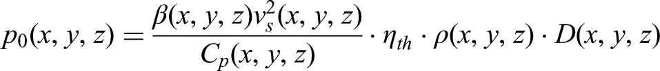
The coefficient of volume expansion β, speed of sound versus, density ρ and specific heat capacity C_p were taken from the literature, and their values are shown in Table 1.^23,24 All parameters are reported for normal physiological conditions. For lack of better values, the efficiency with which absorbed dose is converted into heat, η_th, is assigned a value of unity. The US transport software k-Wave ²⁵ was then used to model the propagation of this initial wave p₀(x,y,z) through the patient model. Briefly, k-Wave is a MATLAB (The Mathworks, Nantucket, PA) and C++ software toolbox designed for the simulation of acoustic wave fields, and particularly for ultrasound applications. It is based on a numerical technique called the k-space pseudo-spectral method, ²⁶ which allows for the efficient and accurate modeling of wave propagation in complex heterogeneous media. k-Wave can simulate a wide range of wave phenomena, including ultrasound and heat transfer, by solving the full time-domain wave equations. We refer the interested reader to the above given references for a more complete description of the capabilities of this software package. The sensor is modeled as a plane of dimensions 20 cm×20 cm with a total of 256 sensing points evenly distributed on it, and this plane is placed at the closest possible distance from the patient model on the anterior side of the body. As the patient surface is not planar, there were several gaps present, which were filled with a water-like coupling medium. The coordinates of each sensing point are assumed to be known with respect to the frame of reference, as are the position of both the x-ray source and the x-ray imaging detector.

Table 1.

Acoustic Parameters for the Several Different Materials Used to Model the US Propagation Through Both the Prostate and Lung Patients. Values are Given for Normal Physiological Conditions.

Material	Sound Speed (m/s)	Heat Capacity (J/kg-K)	Thermal Exp (x 10−4 K−1)
Skin	1624.00	3886.00	3.00
Soft tissue	1545.00	2372.42	2.08
Heart muscle	1561.29	3686.00	2.08
Cortical bone	3514.86	1312.83	0.22
Conn. tissue	1545.00	2372.42	2.08
Lung (inflated)	949.29	3886.00	2.08
Lung (deflated)	1500.00	3886.00	2.08
Water	1482.30	4178.00	2.10
Gold	3240.00	125.40	0.42

XACT Image Reconstruction

Several different reconstruction algorithms for XACT exist, such as the universal reconstruction algorithm, ²⁷ iterative algorithms ²⁸ and time reversal methods. ²⁹ In this work, we used the time reversal method as implemented in the k-Wave toolbox. Unlike Fourier-based algorithms, the time-reversal method does allow for the reconstruction in complex heterogeneous media and is perhaps the most exact reconstruction algorithm currently available. ³⁰ However, in the case of FM XACT localization, it is not realistic to assume that the exact material composition, the geometry, and the location of internal structures are known: if they were, there would be no need to use fiducial markers to localize the target in the first place. Therefore, this information is not available for the reconstruction process so the approximation must be made that the patient is composed of a homogenous medium and the only information used in the reconstruction process is the US signal detected by the sensors. We emphasize that such a signal, as it should, was calculated with the full patient models described above and that it is only in the reconstruction phase of the process that the patient is approximated by a homogeneous, water-like medium with the same external contour as the full patient model. We initially hypothesized that if distortions should arise in the resultant XACT images of the fiducial markers, the x-ray radiograph obtained during the irradiation process would help to correct them, at least partially. As will be shown, this was not necessary. Acoustic signals generated and propagated by k-Wave are deterministic and lack the noise component associated to the actual process of acoustic signal detection, so noise must be added to achieve a more realistic result. Considering the large signal gradient between the background tissue and the gold markers, 15 to 20 times as will be seen later, and the typical noise level of commercially available transducers, in the order of 10 mPa, ¹⁰ a signal to noise ratio of 10 dB was considered appropriate for our work, and the added noise is Gaussian and random in nature. In general, simulations with higher noise levels did not produce significantly different results, due to the aforementioned large difference between the markers and the background signals. This noise-contaminated signal was then fed into the time-reversal reconstruction algorithm of k-Wave using the homogeneous phantom as the propagation medium assuming a US propagation speed of 1540 m/s. The simulation of the initial p₀(x,y,z) transport and subsequent tomographic reconstruction took between 48 and 240 h on a Pentium V 3.5 GHz CPU working within the MATLAB environment. Typical RAM requirements for the 200 µm resolution run in our work ranged from 96 GB to 196 GB. For the lung test case, to further evaluate the robustness of the reconstruction process in a homogenous medium, reconstructions were also carried out by using the lung density in the deflated state with the acoustic parameters of Table 1 for this physiological state. Note that although the lung tissue parameters were changed, the lung volume remained the same, as no CT images at different stages of the respiratory cycle were available. Nevertheless, the simulations are useful and offer insight into what happens when density of lung between inflated and deflated states.

Fiducial Marker Coordinates Extraction

To isolate the markers from the background tissue signal, advantage is taken of the fact that a large gradient exists between the acoustic pressure generated in the FM and the background. A threshold value of 10% of the maximum reconstructed pressure value was used, ie, pressure values less than 10% of the maximum pressure, which is located invariably in the FM, were set to zero, thus isolating the reconstructed p₀(x,y,z) of each marker. Once this is done, the FM appeared in the reconstructed image as a well-defined cluster of points. For each of these clusters, a simple center of mass calculation was then performed to find the coordinates of each FM geometric center. These coordinates were then compared to the true coordinate values of the FM digitally added to the patient model. For each patient model, three sets of simulations were run, each with the three FM at different positions within the tumor.

Results

For each patient model, we only show the simulation that yielded the worst localization of the FM in terms of the center-to-center distance between the reconstructed and the true markers. No dependance of the results in terms of the location of the FM within the tumors was observed, and in general the difference in the reconstructed positions was minimal among the sets of three markers for the same patient model. Again, the absorbed dose in each patient was normalized to an average of 1 mGy over the whole irradiated volume excluding the markers.

Localization of FM in the Lung Patient Model

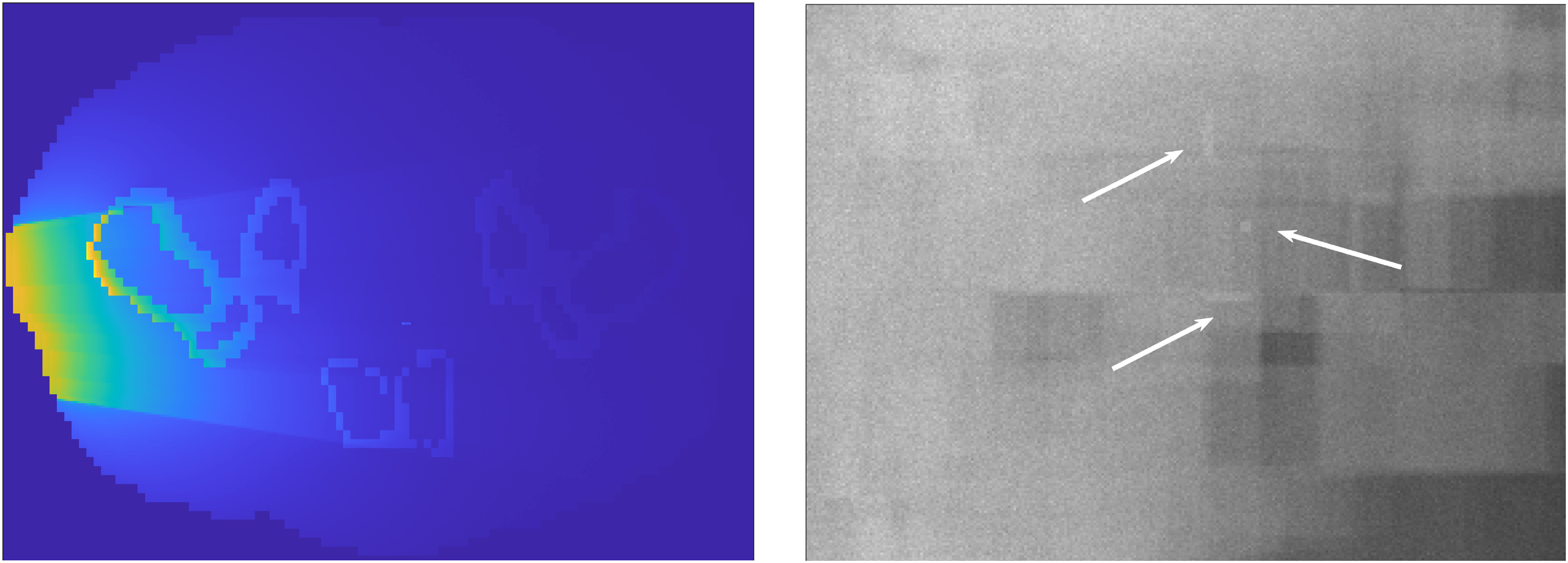
A cross-sectional view of the Monte Carlo calculated initial absorbed dose distribution, is shown on the left panel of Figure 2. The radiological shadows of the markers are clearly visible in the form of horizontal bands indicating a lower absorbed dose at points beyond the markers. The right panel of Figure 2 shows the Monte Carlo calculated radiograph as registered by the imaging detector depicted in Figure 1, with the three markers clearly visible, all with their long axis parallel to each other. The center-to-center distance between each pair of markers for this particular test case were 0.93 cm, 1.54 cm, and 0.71 cm, for the other two test cases the separation between markers were larger.

Figure 2.

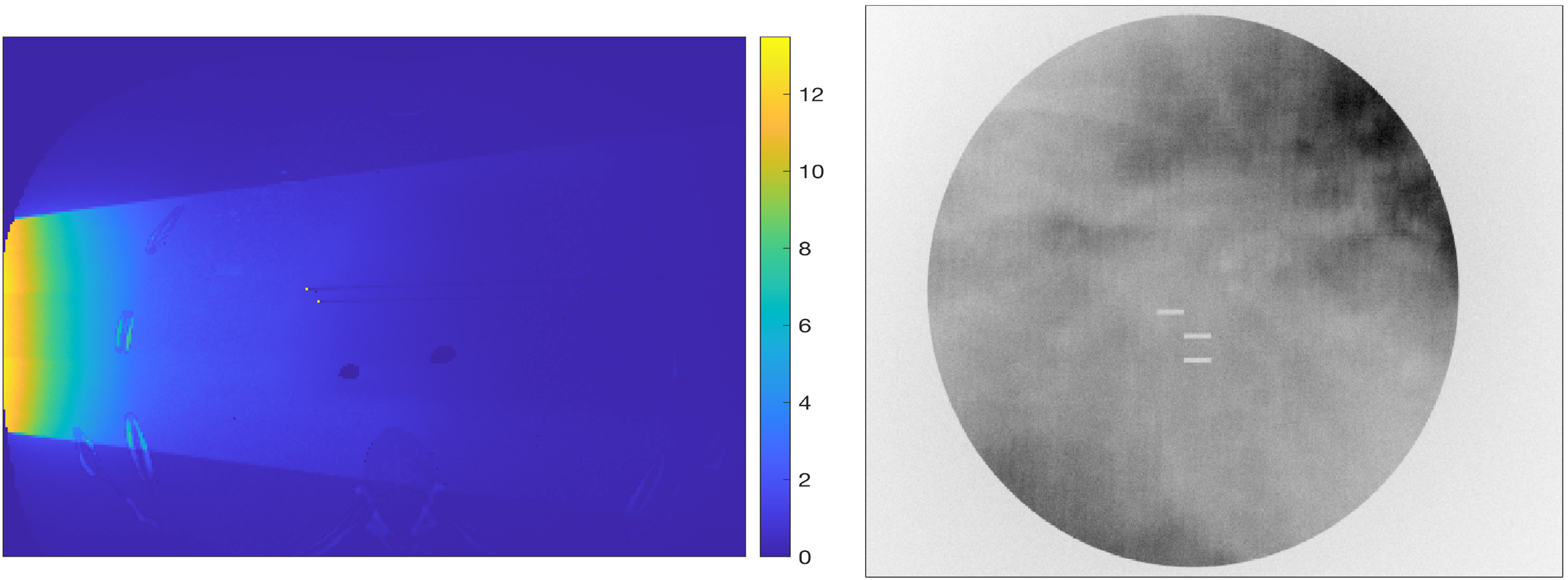
Left Panel: Absorbed Dose Distribution in the Lung Patient Model. The Color Bar Units are in mGy. Right Panel: Monte Carlo Calculated Radiograph Showing the Three Fiducial Markers.

The maximum dose in the FM is in the order of 14 mGy, resulting in a maximum pressure of 954 Pa, a value readily detectable with current commercially available US sensors. Figure 3 shows a 3D visualization of the reconstructed markers, where negative pressure values in the reconstructed matrix have been all set to zero. The left panel of this figure shows the reconstructed initial pressure p0 before applying the threshold mask to isolate the FM, which are shown on the right panel after the threshold was applied. The markers have a jagged appearance, but their rectangular cylindrical shape is still discernible.

Figure 3.

Left Panel: Reconstructed Lung FM Without Thresholding; Right Panel: Image with the 10% of the Maximum Pressure Threshold Applied to Isolate the Markers.

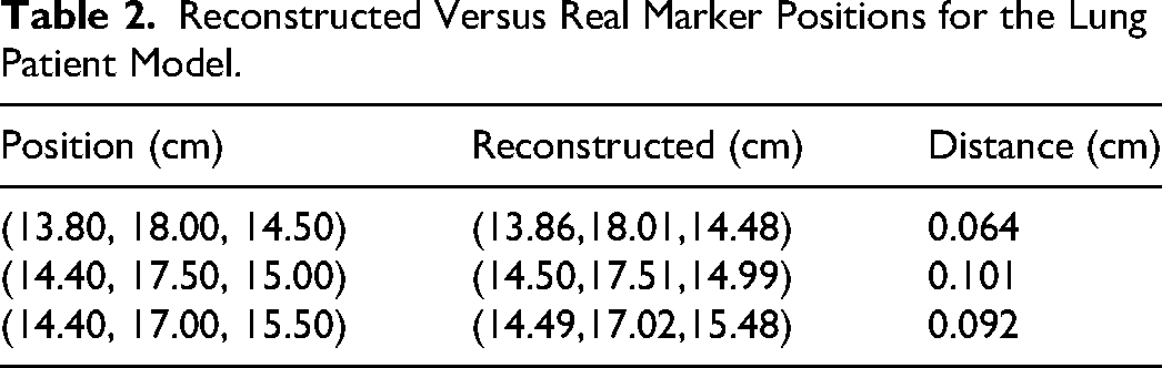
Figure 4 shows a volumetric superposition of the reconstructed and real FM on the same coordinate grid. Note that for the reconstructed markers what is being shown is the points in the reconstructed image whose pressure values exceed the 10% of the maximum pressure threshold, regardless of their actual pressure value. Table 2 shows the coordinates of the center of mass of each FM and the corresponding real coordinates of the point where the center of each FM was placed in the patient model. Notice that all the markers localization errors are within 1 mm.

Figure 4.

Left panel: Superposition of the Digitally Added (Solid Bodies) and Reconstructed FM (Discrete Points) on the Same Frame of Reference. Right Panel: Rotated View of the Three FM.

Table 2.

Reconstructed Versus Real Marker Positions for the Lung Patient Model.

Position (cm)	Reconstructed (cm)	Distance (cm)
(13.80, 18.00, 14.50)	(13.86,18.01,14.48)	0.064
(14.40, 17.50, 15.00)	(14.50,17.51,14.99)	0.101
(14.40, 17.00, 15.50)	(14.49,17.02,15.48)	0.092

As mentioned before, the reconstructed markers have jagged, irregular shapes. This distortion is due to the use of a homogenous medium to approximate the unknown internal geometry and material composition of the patient.

To illustrate this, reconstructions were carried out using the true material composition for this patient and using the sensor readings with the same level of added noise as for the previous reconstructions. One such reconstruction is shown in Figure 5, where the cylindrical shape of the markers is now clearly discernible. For this reconstruction, there was no need to calculate the center of mass for each FM, as their coordinates could be visually obtained from the projection of the reconstructed volume onto the three main planes.

Figure 5.

Left Panel: Reconstructed Lung FM Without Thresholding to Isolate the FM. Right Panel: the Same Reconstruction with Thresholding Applied. Both Reconstructions Were Carried out with the True Material Composition for This Patient.

Table 3 shows the reconstructed versus real marker positions when the lung is in the deflated state. Note how the reconstructed position errors are reduced bringing all three markers into the acceptable error range of 1 mm or less. This shows that, for FM localization in lung, the physiological state of the lung may play an important role in the accuracy with which FM are localized.

Table 3.

Reconstructed Versus Real Marker Positions for the Lung Patient Model When Simulating a Deflated Lung.

Position (cm)	Reconstructed (cm)	Distance (cm)
(13.80, 18.00, 14.50)	(13.82,17.98,14.48)	0.035
(14.40, 17.50, 15.00)	(14.43,17.48,14.98)	0.041
(14.40, 17.00, 15.50)	(14.43,16.98,15.47)	0.047

Localization of FM in the Prostate Patient Model

A cross-sectional view of the initial absorbed dose distribution and a Monte Carlo calculated radiograph for this patient are shown in Figure 6. In the radiograph, it is more difficult to visualize the FM as the beam must travel through the femoral heads on its way to the x-ray image detector, thus losing a sizable portion of the x-ray fluence. The separation between each pair of markers for this particular test case, again measured from center-to-center, were 1.85 cm, 1.76 cm and 1.30 cm. Note also that one of the FM has its long axis running parallel to the incident x-ray beam.

Figure 6.

Left Panel: Absorbed Dose Distribution in the Prostate Patient. The US Sensors are Placed in the Anterior Side of the Patient. Right Panel: Monte Carlo Calculated Lateral Radiograph Showing the Three FM.

For this patient model the maximum absorbed dose in the FM is 15.2 mGy, resulting in a maximum initial pressure of 1 kPa. Figure 7 shows a 3D visualization of the reconstructed markers with and without the 10% thresholding applied to isolate them. One of the markers looks smaller than the others, which is precisely the one with its long axis parallel to the x-ray bream central axis, showing an incomplete reconstruction due to the large attenuation of the x-ray beam along this marker long axis. While this may indicate a possible limitation to the use of XACT as a localization technique, it must be kept in mind that what is of interest is not the visual appearance of the FM but rather the coordinates of their geometric center.

Figure 7.

Left Panel: Reconstructed Lung FM Without Thresholding. Right Panel: Same Reconstruction but with the 10% of the Maximum Pressure Threshold Applied to Isolate the Markers.

As was the case for the lung patient, the appearance of the FM is also jagged and irregular in shape, but the cluster of points is well defined and can be easily discerned to be rectangular cylinders, except for the marker whose long axis runs parallel to the x-ray beam central axis. Figure 8 shows a superposition on the same frame of reference of the reconstructed and real FM, where again, what is shown is only those points whose reconstructed pressure value exceeds the threshold, regardless of their actual magnitude. Despite being an incomplete reconstruction, the points belonging to the partially recovered marker seem to be evenly distributed in the central region of the real marker.

Figure 8.

Left Panel: Superposition of the Digitally Added (solid bodies) and Reconstructed FM (Discrete Points) for the Prostate Patient. Right Panel: Rotated View of the Image in the Left, the Vertical Marker is the One Whose Axis is Parallel To The X-Ray Beam Central Axis.

Table 4 shows the reconstructed FM coordinates compared to the actual coordinates of the markers embedded in the patient model, again obtained by calculating the geometric center of mass of all the points exceeding the 10% of the maximum pressure threshold. All differences are well within 1 mm, with the same results obtained for the two other sets of simulations carried out, and the largest error occurs for the FM parallel to the x-ray beam central axis.

Table 4.

Reconstructed Versus Real Marker Positions for the Prostate Patient Model.

Position (cm)	Reconstructed (cm)	Distance (cm)
(5.20,21.40,15.40)	(5.20,21.41,15.35)	0.049
(7.00,21.80,15.60)	(7.00,21.80,15.61)	0.007
(6.20,22.80,15.80)	(6.19,22.78,15.74)	0.060

Discussion

The ability to accurately localize the reconstructed markers depends on whether the markers can be isolated from each other in the reconstructed XACT images, as in general, their reconstructed images will not be well defined in shape, as can be seen in Figures 3 and 7 above, at least when the reconstruction is carried out using a homogeneous medium instead of the full patient model and using detectors located on the same plane. The resultant acoustic CT images are of poor quality because of two factors: a) the irradiation is taking place using a single x-ray beam, the single-shot, which even if the patient composition were homogenous, would result in acoustic CT images seriously degraded as the x-ray beam entrance side of the patient would look much brighter than the exit side, which is evident on the left panels of Figures 2 and 6, and b) the acoustic signal is registered with all the sensors located on the same plane, a necessity in order to try to keep these sensors from interfering with the therapy beam on its way to the patient. However, and in spite of this, it has been shown that by focusing on the large gradient between the acoustic signal generated by the markers and the surrounding medium, it is still possible to accurately determine the position of the source or sources of this large acoustic signal, and this has been done for two completely different treatment sites, one where the tumor is embedded in a fairly uniform medium and the other when the tumor and the surrounding medium have different acoustics characteristics. Furthermore, as implemented, the acoustic CT images are not even necessary as the reconstruction script automatically localizes the maximum signal in the 3D image matrix, applies the 10% signal threshold (all voxels with a signal less than 10% of the maximum are set to zero), and then proceeds to calculate the center of mass for each cloud of remaining non-zero voxels), with the outcome being the coordinates of each marker.

For the lung patient model, it was shown that the localization error depends on where the lung is located within the respiratory cycle, with larger errors, in the order of 1 mm for one of the markers, when the lung is completely inflated, as in this state the lung density and speed of sound are significantly different from those of the homogeneous medium used in the reconstruction process. The presence of the rib cage does not seem to introduce significant discrepancies, as can be inferred from the fact that for the deflated lung, with a density and speed of sound closer to those of the reconstruction medium, the localization absolute error is in the same range as what was observed for the prostate patient, for which, as shown in Figure 1 and on the left panel of Figure 6, the ultrasound does not traverse any significant bone tissue on its way to the detector. Furthermore, when the full lung patient model was used in the reconstruction process, the distance between the reconstructed and real FM decreased from 0.1 cm to 0.06 cm for the worst-case scenario, confirming that the use of a homogenous medium for the reconstruction of the acoustic signal is the main source of error in the localization process.

Because for the prostate patient model the markers are surrounded by mostly homogenous soft tissue, the deleterious effect of using a homogenous phantom for the reconstruction of the FM is less of a problem: the largest discrepancy was obtained for the FM whose long axis runs parallel to the x-ray beam central axis, as the attenuation of the x-ray beam is substantial in this case, leading to a highly non-uniform dose distribution within the marker, but even in this case, the error is well within the 1 mm acceptable margin.

While it has been shown that it is in principle possible to accurately localize gold FM with a single-shot XACT and without knowledge of the complex internal geometry and material composition of the patient, the purpose of this work was to show feasibility of fiducial marker tracking, and FM localization does not imply tracking, unless the localization is done in a continuous manner. The problem with current methods that truly localize fiducial markers, ie those that directly measure the coordinates of the markers without relying on the observation of external surrogates to infer where the markers are, is that they invariably rely on two radiographic projections which, for a gantry-based treatment machine with imaging x-ray tube and detector mounted opposite to one-another, the treatment delivery process would have to be interrupted to position the gantry for the second x-ray projection. In these systems the two-projection method is only useful for patient positioning, but not for marker tracking. We believe that single-shot photoacoustic tomography can potentially solve this problem because the x-ray projection needed to generate the photoacoustic signal can be obtained regardless of the gantry angle, with the caveat that the treatment beam would have to be briefly interrupted to use the imaging x-ray beam to generate the acoustic signal. This interruption however can be brief as, depending on the power of the imaging x-ray source, pulses of 50 to 100 ns are needed to generate the ultrasound pressure wave. Gated VMAT and other treatment modalities already require the treatment beam to be turned off, so this requirement is not really a burden imposed by the proposed method, and it would have to be experimentally confirmed if indeed it is necessary to turn off the therapy beam, as in principle the pulsed temperature increase would occur against a background temperature, the one produced by the therapy beam, that is fairly constant in time.

One challenging aspect of using XACT as a fiducial marker localization tool is the long reconstruction times, which for the test cases presented in this work ranged from 2 to 5 days on 3.5 GHz processors. Memory requirements are also high, in the order of 100 to 150 GB depending on the problem size, as the resolution required to achieve a meaningful frequency must be in the order of 200 µm or higher. Reconstruction times must be in the order of a few seconds if actionable information is to be extracted from the tracking of the FM. To this end, it is necessary to evaluate whether using a smaller patient volume, therefore reducing the number of voxels in the reconstruction process, would yield the same accuracy as that obtained with the full volume. Alternatively, a massively parallel computing equipment can be used to speed up the reconstruction process. ³¹

Conclusions

Using Monte Carlo simulation and realistic patient models, it has been shown that single-shot x-ray acoustic tomography can potentially be and effective tool for the localization and tracking of radiotherapy fiducial markers, exhibiting an accuracy of better than 1 mm, despite the poor visual quality of the resultant images. It was also shown that this accuracy can be achieved despite using a homogeneous body to approximate the unknown internal geometry and material composition of the actual patient, thus making the technique fully compatible with the challenging clinical problem of radiotherapy fiducial marker localization. For markers located in lung tumors, the tracking error is larger when the lung is in the inflated state, as in this case its density and speed of sound differ substantially from those of the homogeneous medium used in the reconstruction process.