
Abstract
Introduction
Background
Image-guided radiation therapy (IGRT) has experienced considerable advancements since the development and implementation of onboard cone-beam computed tomography (CBCT) systems. 1 Recently, radiation therapy systems with integrated MRI scanners have been introduced clinically providing superior soft-tissue contrast compared to X-ray-based imaging. 2 In addition to RECIST and other similar protocols based on visible tumor measurements [https://recist.eortc.org/], computed tomography (CT), positron emission tomography (PET), and magnetic resonance imaging (MRI) images are qualitatively analyzed by radiologists as a standard practice for screening, staging or decision-making purposes. 3 Quantitative analysis, or radiomics, aims to extract additional information from these standards of care images with the hypothesis that texture and voxel value distribution contain physiological information not discernable visually. 4 Images are converted into mineable data generating so-called radiomics features (imaging biomarkers) relating to pathophysiological processes which, combined with other patient data, are hypothesized to provide predictive or discriminative information.4-6 By combining qualitative and quantitative data, the long-term goal is to build reliable descriptive clinical models, tailoring treatment to each patient and provide even further personalized oncology than available today.7-9
Quantitative image analysis can be divided into several steps: image acquisition, segmentation, feature extraction, statistical analysis, and model building, each with unique challenges.5,8,10 Features can be vulnerable to differences between and within image modalities such as fundamental imaging physics, imaging parameters, reconstruction methods, a segmentation method, feature extraction software, etc.8-12 Comparison between institutions is therefore difficult and the lack of standardized methodologies is a major challenge for radiomics to overcome before clinical translation.5,8,9 Furthermore, models based on nonrobust features will likely not provide reliable predictions when applied prospectively to new data. 13 Although no standardized guidelines on how to assess feature robustness have been developed, it is emphasized by The Image Biomarker Standardization Initiative (IBSI) 6 as a primary step in the feature selection process. 14 IBSI is an independent international collaboration aiming to establish common biomarker nomenclature and definitions for the radiomics community. Thus, identifying features that are robust under various imaging conditions is essential to develop clinical outcome prediction or clinical decision support systems.5,14
ViewRay's MRIdian MRI-Linac (ViewRay Inc., Cleveland, OH) is a commercially available hybrid system combining a 0.35T scanner with a 6 MV flattening-filter-free (FFF) medical electron linear accelerator. 15 This system provides a potentially advantageous setting in which images for radiomics analysis are acquired within the context of radiotherapy treatment on a daily basis. However, reliable approaches and robust radiomics features acquired with this MRI-guided radiotherapy (MRIgRT) workflow still remain to be determined. In this retrospective study, we investigated radiomics features in both phantom and patient images acquired with the scanner of such a system, with a primary focus on robustness assessment, investigating the repeatability and reproducibility of the system and associated radiomics feature calculations. The aim was to explore longitudinal radiomics studies in invariant objects as well as identifying robust radiomics features across various imaging conditions. Additionally, a literature review over MRI-based radiomics with emphasis on either assessing robustness or various clinical correlations was included in this work for comparison, and to identify potential features fulfilling both the robustness and predictive criteria.
Literature Review
The main aim of this work was to investigate feature variability and performing a robustness assessment of the integrated MRI-Linac system in both phantom and patient data. A literature review with the purpose of providing a comprehensive summary of other available similar studies within MRI-based radiomics was included. The main literature collection took place between January and May 2020, but a few later published papers have been included after this. Most literature14,16-28 was found through the PubMed database searching for, for example, “MRI radiomics,” “MRI Linac radiomics,” “MRI radiomics stability,” “Radiomics phantom study,” etc. A summary of published studies with similar questions, aims, or other relevant findings regarding feature variability based on their relevance to our study were therefore included. The primary goal was to characterize robust features in various imaging conditions. It is important to recall that feature robustness is not an implication of feature predictability or other biomarker correlation to any clinical task or outcome. 14 A secondary goal of the literature review was therefore to identify common radiomics features demonstrating both high robustness and significant clinical correlation. Thus, a summary of the relevant papers included in the literature review can be seen in Tables 1 and 2, where the study purpose, feature classes, and robust/predictive features consistent with the findings in this work are presented.
Summary of MRI-Based Radiomics Robustness Assessment Papers.
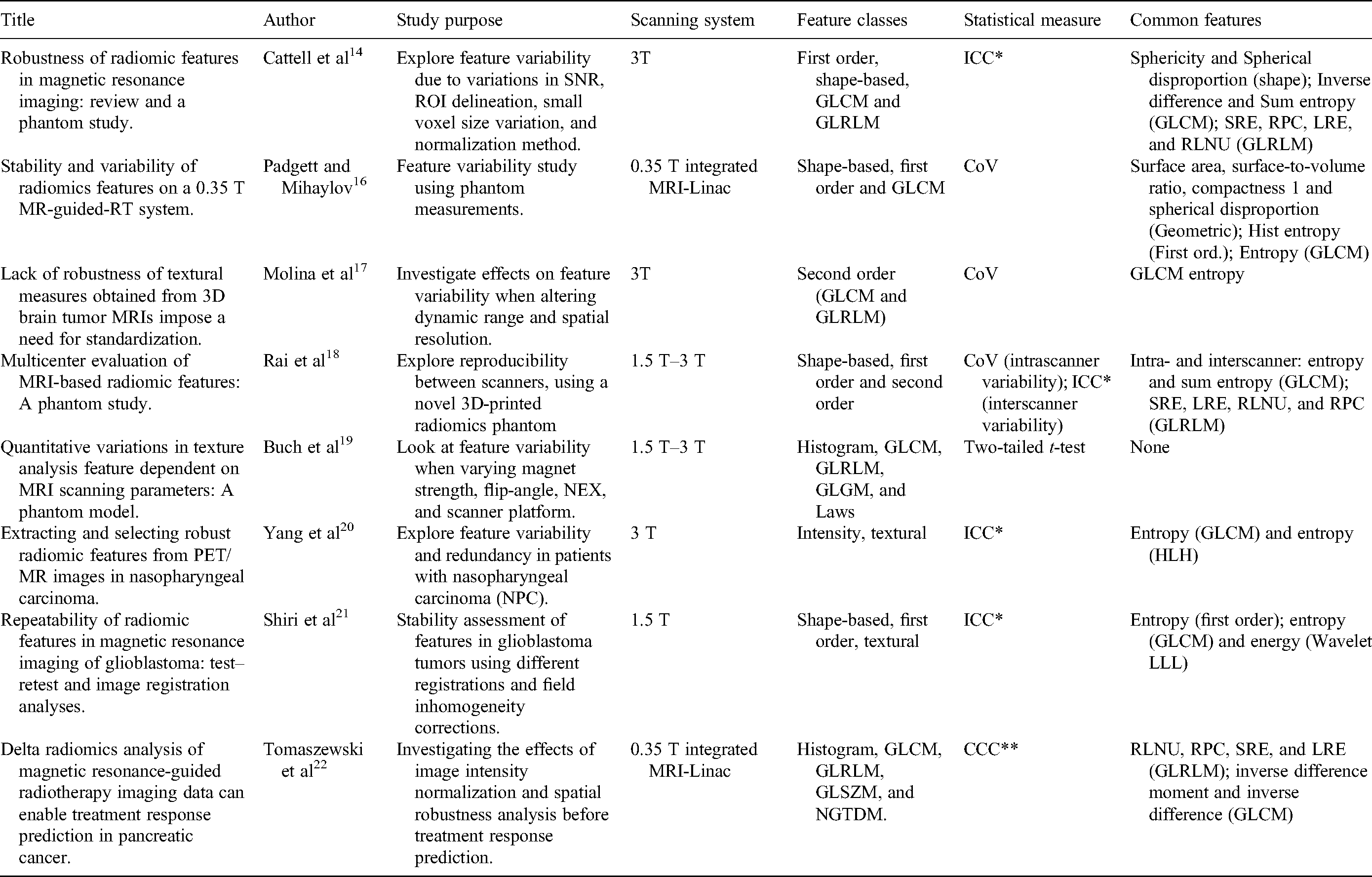
Summary of MRI-Based Radiomics Looking at Various Clinical Correlations.

Materials and Methods
Phantom Properties
The Magphan®RT Phantom (Figure 1) consists of 2 parts: a top module (TMR009) and a bottom module (TMR007). Both contain >100 spherical fiducials and other solid test components filled with an MRI-signal generating liquid (96.4% distilled water, 2.5% PVP, 0.9% sodium chloride, <0.2% potassium sorbate, <0.2% copper sulfate, and <0.2% blue food color, all defined in percentage by weight). This results in T1 and T2 values of about 175 to 225 ms at 0.35 T.29,30
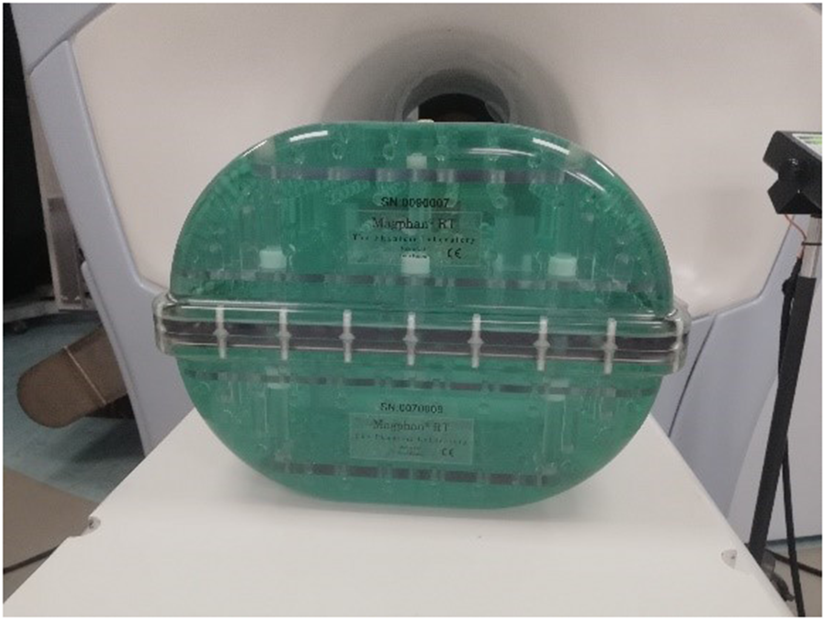
Magphan® RT phantom.
The ViewRay Daily QA Phantom (Figure 2) is a cylindrical phantom filled with distilled water. It has 1 central and 4 surrounding cavities for insertion of an ionization chamber. 31

ViewRay Daily QA phantom.
Data Selection
Eleven scans acquired over a 13-month period using the Magphan®RT Phantom, and acquired over 11 workdays using the ViewRay Daily QA Phantom, respectively, constituted the complete phantom dataset.
The Institutional Review Board at the University of South Florida approved (IRB #20383) and waived the informed consent requirement for retrospective analysis in this study. Patient data included 50 images from 10 anonymized stereotactic body radiation therapy (SBRT) pancreas cancer patients treated with 50 Gy in 5 consecutive daily fractions. The kidneys and liver were chosen to represent theoretically invariant objects in the patient, assuming no significant effect of radiation during the course of treatment and consistent distance/orientation relative to the pancreatic target, thus ensuring consistent location within the imaging coils. Both organs exhibit a desirable heterogeneity for radiomics studies, thus being appropriate alternatives as a transition from ideal imaging conditions to more complex structures as human tissue.
In summary, 4 datasets were included for statistical analysis of calculated radiomics features defined as follows: monthly phantom, daily phantom, patient kidney, and patient liver.
Image Acquisition and Registration
All phantom images were acquired using a torso coil and high-resolution TRUFI pulse sequence with imaging parameters: 1.5 mm × 1.5 mm × 1.5 mm resolution, 500 mm × 449 mm × 432 mm Field of View (FOV) and 172 s total image acquisition time. Positioning and set-up were identical for every scanning occasion. All patient images were acquired using a torso coil and TRUFI pulse sequence with 1.5 mm × 1.5 mm × 3.0 mm resolution, 540 mm × 465 mm × 432 mm FOV and 25 s total imaging time (for faster imaging during treatment). Image export, import, segmentation, and registration were done in Mirada RTx (Mirada RTx 1.6, Mirada Medical, Oxford, UK).
Identical cylindrical 4.2 cm3 VOIs were contoured in different sections of both phantoms: 4 regions in the Magphan®RT Phantom (Figure 3) and 2 regions in the ViewRay Daily QA Phantom (Figure 4). All structures were propagated from the baseline to the remaining ten imaging sets by rigid registration in Mirada RTx. For each patient image a spherical 14 cm3 VOI was placed in the midsection anteriorly/posteriorly, 4 cm caudally from the diaphragm, and 11 cm laterally from the aorta (Figure 5b), while kidneys were manually segmented by a single user (Figure 5a).

(a)-(d) Four cylindrical VOI were placed in various regions in the Magphan® RT phantom displaying heterogeneous patterns.

(a), (b) Two VOI of the same size were placed in the ViewRay Daily QA phantom.

(a) Kidneys were manually segmented for each patient image, (b) a spherical VOI was placed in the liver for each patient and scanning occasion.
Statistical Analysis
Traverso et al 3 defined feature robustness into 2 main elements: repeatability and reproducibility. Repeatability refers to the agreement between measurements under identical imaging conditions, that is, intrasubject scanning using identical scanning parameters, set-up, equipment, etc. Reproducibility refers to the degree to which features stay unchanged under various imaging conditions, for example, identical imaging parameters but different subjects, different imaging parameters but the same subject, etc. In this study, features fulfilling both of these requirements were classified as robust.
In this work, the CoV was chosen as the figure of merit for robustness quantification since it allowed for a straightforward methodology to identify robust features within and between many subjects. It is defined as
Feature Extraction and Statistical Workflow
An in-house program, whose definitions are based on IBSI recommendations and those found in the work by Shafiq-ul-Hassan et al,
9
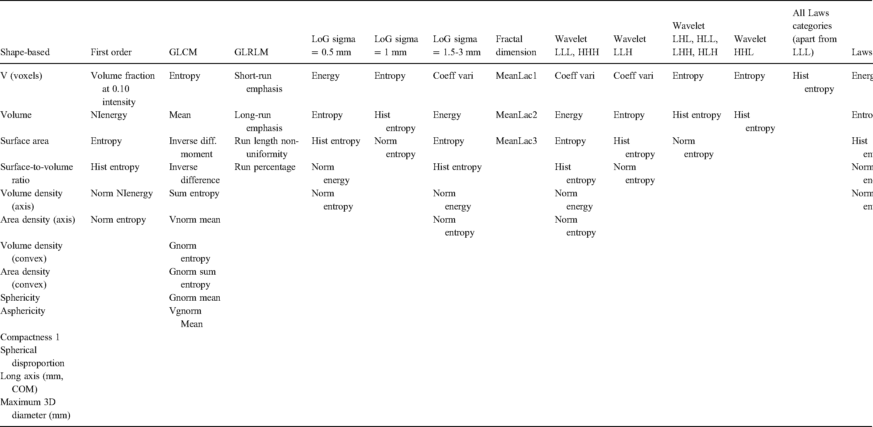
was used to extract 1085 shape-based, first, second, and higher-order features (Table 3). Shape-based features describe various geometric properties of the VOI, such as volume, compactness, surface area, etc.6,10 First order features relate to voxel intensity distribution within the VOI, with no regard to their relative spatial distribution.
5
Most of these features require intensity discretization of the 2D or 3D data before calculation.6,10 Second-order statistics, also referred to as texture features, provide both intensity and spatial information. They describe the distribution of voxel intensity values between neighboring voxels along with different directions and distances and are derived from so-called
Complete Summary of Feature Sub-Categories, Number of Extracted Features are Written Within Parentheses.

Repeatability and reproducibility were assessed with CoV < 5% as the threshold for feature robustness. Feature extraction was carried out for all imaging sessions and VOIs in each patient/phantom, followed by calculation of CoV. For both phantom datasets, each VOI was initially treated separately. The mean value of CoV for all VOIs (4 VOIs in the monthly phantom dataset and 2 in the daily) was then evaluated and robust features (CoV < 5%) in each dataset were identified. A similar initial feature selection procedure was applied to the patient kidney and liver data, respectively, calculating CoV for all features in each individual patient dataset first. Robust features were then identified by looking at the CoV mean between all patients within the kidney and liver datasets separately. Features fulfilling the robustness criteria in all 4 datasets were selected in the final step. Thus, the statistical workflow took into account both the repeatability and reproducibility criteria by looking at intrasubject variability in the first step, followed by intersubject analysis between different patients and as well in the final feature selection process.
Results
In this study 130 out of 1085 radiomics features demonstrated high robustness in both phantom and patient data. Robust features were identified in every category apart from GLSZM and NGTDM. All final robust features (CoV < 5%) are presented in Table 4 and quantitative results are presented in Appendix (Table 6). Out of the 130 features that we identified, 17 were characterized as robust in the literature review while 13 features were found to have significant discriminative or predictive power in various clinical tasks mentioned in the literature (see Table 5). Features found to be both robust and predictive in the literature are marked in bold. The textural feature
Selected Robust Features (CoV < 5%) in Both Phantom and Patient Data Sorted by Sub-Category.
Robust Features Fulfilling the Robustness or Predictive Criteria in the Chosen Literature Review That are Common to Our Result. Features Marked in Bold are Found to be Both Robust and Predictive in the Literature.

Note: The code to compute radiomic features used in this paper can be shared upon request.
Discussion
Our literature review included both phantom and patient data analysis, as well as different approaches to investigate reproducibility and repeatability. Cattell et al 14 performed phantom measurements looking at variability due to altering signal-to-noise ratio (SNR), ROI delineation, small voxel size variation, and normalization methods. They concluded that many features are nonrobust over these variations. The work by Rai et al 18 used a 3D-printed phantom for exploring intra- and inter-scanner variability. They identified robust first order and texture features but also reported an overall noticeable variation in feature robustness. The phantom study by Buch et al 19 looked at the effect of varying magnet strength, flip-angle, number of excitations (NEX), and scanner platform and found no features that were stable across all alterations. Although results varied among peer-reviewed papers, most authors agreed that many features are sensitive to several external factors and that further research in order to understand their behavior is essential.
Several studies explored novel methods of designing MRI texture radiomics phantoms. Rai et al 18 designed a 3D-printed phantom and Buch et al 19 constructed a phantom using doped gel-filled tubes. Valladares et al 43 presented a summary of various MRI texture phantom analysis studies in which different materials for simulating tumor heterogeneity were used. Most designs consisted of solid structures, usually polystyrene spheres or porous foams embedded in an agarose gel mixture. However, limitations regarding sensitivity to temperature and humidity are 2 factors to be overcome before handling these in multicenter trials. The phantoms in our work were designed for QA and consisted of homogeneous structures giving rise to a close to a binary signal. Prospective research would be to expand our analysis to texture phantoms similar to those found in the literature mentioned.
Radiomics is a fast emerging area and several studies on the subject have therefore been published since the time of our literature review. Sun et al
44
presented a recent phantom study on robustness analysis of images from a 1.5 T scanner of an integrated MRI-Linac. Like our results, they found a significant effect on feature variability from the test–retest cohort and therefore emphasize the importance of removing features that are sensitive to machine influence. No common robust features were identified between their work and ours. In another phantom study by Wong et al,
45
they investigated longitudinal feature repeatability on two 1.5 T scanners by acquiring 30 consecutive daily images of an ACR MRI phantom. Five of their repeatable shape-based features overlapped with our results, namely: maximum 3D diameter, sphericity, surface area, surface-to-volume ratio, and voxel volume. It should be noted that
We used an in-house developed program, based on the definitions given by IBSI, for feature extraction. However, studies show that features might be vulnerable to the choice of extraction software since calculation settings can vary.12,47 Fornacon-Wood et al 47 compared the outcome between 4 platforms, 3 of which were IBSI-compliant, and concluded that choice of the program has an effect on feature variability as well as their correlation to clinical outcome. In the work by McNitt-Gray et al, 12 they looked at the agreement between different radiomics software packages under controlled conditions using standardized radiomics feature definitions (using the IBSI manual). They concluded that high levels of agreement between packages were achieved for some of the features while feature definitions requiring more complex derivations did not show the same levels of agreement. Thus, although standard definitions are being used, the choice of feature extraction software has an impact on the final determination, which should be taken into consideration when analyzing and comparing results. There is progress towards reaching common ground, but variations are still prevalent and remain a challenge for radiomics studies.
Another limitation to our analysis lies in the choice of cylindrical and spherical VOIs for phantom and patient (liver) data, respectively. These shapes do not have any unique long or short axis, which is of relevance for calculating many of the shape-based features. Volume and area are not affected but it is worth considering that some shape-based features may lose their meaning in these datasets.
Gray-level normalization is recommended11,20,21,25 before feature extraction and analysis to reduce the effects of using different scanners, protocols, and reconstruction parameters. As concluded by Lacroix et al 25 image processing correcting for, for example, magnetic field inhomogeneity or voxel value normalization are 2 of numerous aspects shown to affect feature outcome. The effect of gray-level normalization is further emphasized by Collewet et al. 11 In our study each dataset was acquired with the same scanner and protocol. Since each dataset was analyzed separately before identifying common robust features among all data, normalization was omitted as it was assumed that the system produced similar images under the same imaging conditions. In fact, our robustness analysis is temporal to discern the potential effects of scanner drift on feature robustness. Interestingly, a recent study on a similar 0.35 T MRI-Linac system by Tomaszewski et al 22 looked at treatment response prediction for delta radiomics in pancreatic cancer patients and concluded that normalization reduces interscan signal variations as well as nonpathologic signal drift. They emphasize the importance of image preprocessing and robustness analysis before feature selection and present an explicit normalization method. We acknowledge that there may be many preprocessing techniques to improve feature robustness (SNR). Our assumption of no scanner drift is therefore a more conservative approach for the selection of robust features.
Our results indicate that 13 radiomics features overlapped between our analysis and with those identified as predictive/prognostic in the literature review. Boldrini et al 23 looked at a similar 0.35 T MRI-Linac system as in this work whereof 9 common features could be identified. Although preliminary, this is a promising result suggesting a useful potential for radiomics studies on such a system across scanners and institutions. In another study on the same system by Tomaszewski et al, 22 several common features were identified in their robustness analysis, but no overlap was seen between their predictive features and our results; this can be expected since the test for robustness was completely different. The textural feature GLCM entropy has been characterized as a significant classifier for lesion discrimination in several studies as well as in stability assessment papers. The results are promising by identifying radiomics features for further investigation. Although a large number of features were classified as robust in our work, a substantial proportion were not (88%). MRI-based radiomics stability assessment has been investigated but to a limited extent, thus even though efforts are made in finding common methods, no consensus in stating feature robustness or their predictive power currently exists. The situation where features are found to be predictive but not robust must be further investigated. We, therefore, stress the importance of reporting feature variability and further emphasize the relevance of robustness assessment as a first step before starting any useful clinical correlation.
This work has investigated the robustness assessment of a 0.35 T integrated MRI-Linac with respect to derived radiomics features and provides a comprehensive and novel summary of longitudinal radiomics on such a system. We identified 130 robust features and conclude that certain radiomics features on images acquired with the low-field scanner of the system are stable over time. Phantom and human data were analyzed separately as a prior step, while the final analysis entailed a joint comparison and extraction of common robust features, which to our knowledge has not been performed on such a system before. Although no texture phantoms were used that reflect the complexity and wide range of gray levels observed in human tissue, the phantom analysis is valuable for representing ideal imaging conditions in a controlled experimental setting. Combined with patient data it is therefore useful as an indication of variability solely due to inherent machine properties. Thus, it is in our future interest to develop a heterogeneous phantom to further explore and confirm feature behavior on a low-field MRI-Linac.
Conclusion
This work has explored the longitudinal robustness of radiomics features studies on a low-field integrated MRI-Linac and assessed that the 0.35 T scanner of the system is sufficiently stable over time for such analysis. Our results indicate that robust features over a wide range of imaging conditions can be identified in both phantom and patient data, and we emphasize the usefulness of phantom studies for feature stability assessment as it provides a controlled setting. Developing a functional texture phantom for MRI-based radiomics would be of great interest in future studies. Furthermore, a literature review revealed that several of the features demonstrating a high level of stability in our analyses have also been found to be significantly related to various clinically relevant factors.
Footnotes
Abbreviations
MRI, magnetic resonance imaging; SBRT, stereotactic body radiation therapy; TRUFI, true fast imaging with steady state free precession; CoV, coefficient of variation; GLSZM, gray level size zone matrix; NGTDM, neighborhood gray tone difference matrix; IGRT, image guided radiation therapy; CBCT, cone-beam computed tomography; CT, computed tomography; PET, positron emission tomography; IBSI, image biomarker standardization initiative; FFF, flattening-filter-free; MRIgRT, MRI-guided radiotherapy; ICC, intraclass correlation coefficient; CCC, concordance correlation coefficient; SNR, signal-to-noise-ratio; ROI, region of interest; NEX, number of excitations; NPC, nasopharyngeal carcinoma; GLCM, gray level co-occurrence matrix; GLRLM, gray level run length matrix; GLGM, gray level gradient matrix; SRE, short run emphasis; LRE, long run emphasis; RLNU, run length non-uniformity; RPC, run percentage; FOV, field of view; VOI, volume of interest.
Ethics Statement
The Institutional Review Board at the University of South Florida approved (IRB #20383) and waived the informed consent requirement for retrospective analysis in this study.
Declaration of Conflicting Interests
The authors declared no potential conflicts of interest with respect to the research, authorship, and/or publication of this article.
Funding
The authors disclosed receipt of the following financial support for the research, authorship, and/or publication of this article: This work was funded in part by the Crafoord Foundation travel grant (Sweden).
Appendix
The Coefficient of Variation for the 130 Radiomics Features That Were Identified as Robust. Standard Deviation is Written Within Parenthesis.

| Feature category | Feature | Liver | Kidney | Monthly | Daily |
|---|---|---|---|---|---|
| Shape-based | Long axis (mm,COM) | 0.2 (0.09) | 1.6 (0.61) | 0.45 (0.16) | 0.47 (0.01) |
| Maximum 3D diameter (mm) | 0.13 (0.07) | 1.19 (0.5) | 0.37 (0.14) | 0.5 (0.09) | |
| V (voxels) | 0.58 (0.23) | 2.41 (0.87) | 1.37 (0.99) | 0.55 (0.18) | |
| Volume | 0.58 (0.23) | 2.41 (0.87) | 1.37 (0.99) | 0.55 (0.18) | |
| Surface area | 0.73 (0.24) | 1.64 (0.7) | 0.58 (0.07) | 0.52 (0.27) | |
| Surface-to-volume ratio | 0.32 (0.09) | 1.49 (0.54) | 1.19 (1.05) | 0.22 (0.1) | |
| Volume density (axis) | 1.72 (0.89) | 3.25 (1.15) | 3.83 (3.43) | 1.3 (0.93) | |
| Area density (axis) | 1.23 (0.47) | 1.8 (0.43) | 1.51 (0.8) | 0.95 (0.7) | |
| Volume density (convex) | 0.58 (0.25) | 0.79 (0.33) | 1.02 (0.7) | 0.5 (0.15) | |
| Area density (convex) | 0.6 (0.27) | 0.72 (0.37) | 0.4 (0.23) | 0.32 (0.08) | |
| Sphericity | 0.42 (0.09) | 1.04 (0.41) | 0.8 (0.61) | 0.2 (0.19) | |
| Asphericity | 1.28 (0.28) | 2.31 (0.87) | 1.97 (1.53) | 0.48 (0.47) | |
| Compactness 1 | 0.63 (0.14) | 1.56 (0.62) | 1.2 (0.91) | 0.3 (0.29) | |
| Spherical disproportion | 0.42 (0.09) | 1.05 (0.41) | 0.82 (0.64) | 0.2 (0.2) | |
| First order | Volume fraction at 0.10 intensity | 0.45 (0.26) | 0.57 (0.53) | 2.88 (2.24) | 0.3 (0.07) |
| NIenergy | 0.66 (0.35) | 2.71 (0.98) | 2.24 (0.61) | 0.72 (0.26) | |
| Entropy | 0.08 (0.03) | 0.25 (0.09) | 0.34 (0.06) | 0.1 (0.04) | |
| Hist entropy | 2.26 (1.37) | 1.21 (0.47) | 1.59 (0.65) | 1.84 (0.7) | |
| Norm NIenergy | 0.28 (0.23) | 0.61 (0.35) | 1.25 (0.71) | 0.2 (0.08) | |
| Norm entropy | 0.02 (0.02) | 0.03 (0.02) | 0.21 (0.11) | 0.03 (0.01) | |
| LoG sigma = 0.5 | Energy | 0.72 (0.37) | 2.71 (0.93) | 2.15 (0.72) | 0.75 (0.26) |
| Entropy | 0.08 (0.04) | 0.25 (0.09) | 0.35 (0.08) | 0.1 (0.04) | |
| Hist entropy | 1.95 (0.51) | 0.9 (0.47) | 1.01 (0.25) | 1.41 (0.18) | |
| Norm energy | 0.36 (0.28) | 0.65 (0.35) | 1.97 (0.27) | 0.46 (0.13) | |
| Norm entropy | 0.02 (0.02) | 0.03 (0.02) | 0.27 (0.06) | 0.05 (0.02) | |
| LoG sigma = 1 mm | Entropy | 0.21 (0.1) | 0.29 (0.1) | 0.5 (0.09) | 0.58 (0.21) |
| Hist entropy | 2.01 (0.87) | 1.85 (0.92) | 2.63 (0.84) | 3.45 (0.66) | |
| Norm entropy | 0.15 (0.05) | 0.06 (0.03) | 0.34 (0.12) | 0.49 (0.19) | |
| LoG sigma = 1.5 mm | Coeff Vari | 2.06 (1.66) | 1.28 (0.58) | 2.94 (0.8) | 3.01 (0.58) |
| Energy | 1.88 (1.19) | 2.92 (1.08) | 3.01 (0.98) | 3.01 (0.78) | |
| Entropy | 0.21 (0.08) | 0.29 (0.11) | 0.39 (0.1) | 0.35 (0.09) | |
| Hist entropy | 1.89 (0.79) | 1.79 (0.74) | 1.93 (0.18) | 2.17 (0.59) | |
| Norm energy | 1.55 (1.31) | 1.01 (0.46) | 3.04 (1.42) | 2.34 (0.54) | |
| Norm entropy | 0.12 (0.09) | 0.06 (0.02) | 0.33 (0.13) | 0.22 (0.05) | |
| LoG sigma = 2 mm | Coeff Vari | 3.03 (1.77) | 1.68 (0.8) | 2.3 (0.37) | 3.71 (0.31) |
| Energy | 2.45 (1.49) | 3.17 (1.06) | 2.44 (0.8) | 2.86 (0.58) | |
| Entropy | 0.23 (0.12) | 0.3 (0.11) | 0.35 (0.16) | 0.29 (0.04) | |
| Hist entropy | 1.86 (0.7) | 2 (0.9) | 1.08 (0.09) | 1.84 (0.34) | |
| Norm energy | 2.31 (1.38) | 1.36 (0.66) | 2.12 (0.21) | 2.96 (0.37) | |
| Norm entropy | 0.17 (0.09) | 0.08 (0.03) | 0.22 (0.05) | 0.29 (0.02) | |
| LoG sigma = 2.5 mm | Coeff Vari | 3.9 (2.04) | 2.08 (1.12) | 3.77 (0.86) | 4.29 (0.12) |
| Energy | 3.22 (1.88) | 3.45 (1.13) | 3.86 (1.34) | 3.83 (0.48) | |
| Entropy | 0.3 (0.15) | 0.31 (0.11) | 0.53 (0.19) | 0.46 (0.08) | |
| Hist entropy | 2.2 (0.81) | 2.02 (1.13) | 1.44 (0.57) | 2.33 (0.34) | |
| Norm energy | 3.08 (1.77) | 1.76 (0.98) | 3.26 (0.63) | 3.44 (0.07) | |
| Norm entropy | 0.22 (0.13) | 0.1 (0.04) | 0.39 (0.12) | 0.33 (0.03) | |
| LoG sigma = 3 mm | Coeff Vari | 4.33 (2.14) | 2.1 (1.17) | 4.28 (0.81) | 3.41 (0.83) |
| Energy | 3.94 (2.4) | 3.56 (1.33) | 4.6 (1.58) | 3.91 (0.27) | |
| Entropy | 0.37 (0.21) | 0.32 (0.13) | 0.62 (0.22) | 0.51 (0.04) | |
| Hist entropy | 2.22 (0.84) | 2 (1.03) | 1.19 (0.31) | 1.77 (0.11) | |
| Norm energy | 3.52 (1.98) | 1.82 (1.04) | 3.72 (0.9) | 2.72 (0.87) | |
| Norm entropy | 0.27 (0.14) | 0.1 (0.05) | 0.45 (0.14) | 0.27 (0.07) | |
| Wavelet LLL | Coeff Vari | 3.21 (1.21) | 3.08 (1.39) | 2.59 (0.9) | 1.74 (0.62) |
| Energy | 1.41 (0.59) | 3.06 (1.23) | 2.08 (0.38) | 1.33 (0.56) | |
| Entropy | 0.14 (0.06) | 0.28 (0.12) | 0.27 (0.05) | 0.16 (0.06) | |
| Hist entropy | 1.27 (0.92) | 1.12 (0.38) | 1.3 (0.55) | 0.95 (0.41) | |
| Norm energy | 1.39 (0.53) | 1.63 (0.7) | 1.82 (0.72) | 1.04 (0.39) | |
| Norm entropy | 0.13 (0.04) | 0.12 (0.06) | 0.22 (0.09) | 0.11 (0.04) | |
| Wavelet LLH | Coeff Vari | 3.7 (1.63) | 4.55 (1.89) | 3.34 (1.74) | 2.62 (0.89) |
| Entropy | 0.69 (0.27) | 1.13 (0.51) | 0.78 (0.52) | 0.37 (0.15) | |
| Hist entropy | 1.15 (0.48) | 1.4 (0.52) | 0.49 (0.19) | 0.6 (0.16) | |
| Norm entropy | 0.7 (0.27) | 1.13 (0.5) | 0.79 (0.66) | 0.4 (0.18) | |
| Wavelet LHL | Entropy | 1.41 (0.48) | 0.99 (0.44) | 1.17 (0.63) | 0.78 (0.51) |
| Hist entropy | 1.12 (0.51) | 1.62 (0.6) | 0.49 (0.02) | 0.54 (0.06) | |
| Norm entropy | 1.4 (0.49) | 0.96 (0.45) | 1.11 (0.53) | 0.76 (0.48) | |
| Wavelet HLL | Entropy | 1.37 (0.58) | 1.16 (0.7) | 1.24 (1.36) | 0.53 (0.34) |
| Hist entropy | 1.19 (0.33) | 1.24 (0.56) | 0.59 (0.26) | 0.66 (0.24) | |
| Norm entropy | 1.38 (0.59) | 1.09 (0.66) | 1.21 (1.24) | 0.56 (0.37) | |
| Wavelet LHH | Entropy | 2.13 (0.88) | 2.28 (1.01) | 3.24 (2.95) | 1.49 (0.34) |
| Hist entropy | 1.15 (0.48) | 1.46 (0.62) | 0.41 (0.12) | 0.46 (0.16) | |
| Norm entropy | 2.13 (0.91) | 2.24 (0.99) | 3.26 (2.9) | 1.51 (0.32) | |
| Wavelet HLH | Entropy | 2.27 (1.02) | 3.07 (1.09) | 3.09 (1.65) | 3.24 (2.42) |
| Hist entropy | 0.95 (0.5) | 2.13 (0.79) | 0.52 (0.2) | 0.58 (0.25) | |
| Norm entropy | 2.26 (1.02) | 3.08 (1.12) | 3.04 (1.69) | 3.22 (2.39) | |
| Wavelet HHL | Entropy | 1.55 (1.59) | 2.98 (1.4) | 4.99 (6.74) | 0.83 (0.25) |
| Hist entropy | 1.13 (0.39) | 1.22 (0.4) | 0.57 (0.17) | 0.54 (0.19) | |
| Wavelet HHH | Coeff Vari | 3.9 (2.14) | 4.66 (2.59) | 2.59 (1.13) | 1.91 (1.26) |
| Energy | 0.57 (0.27) | 2.64 (1.02) | 1.88 (0.78) | 0.8 (0.42) | |
| Entropy | 0.07 (0.03) | 0.24 (0.09) | 0.24 (0.11) | 0.1 (0.04) | |
| Hist entropy | 1.23 (0.43) | 1.18 (0.46) | 0.56 (0.17) | 0.37 (0.02) | |
| Norm energy | 0.23 (0.15) | 0.47 (0.28) | 0.97 (0.55) | 0.41 (0.27) | |
| Norm entropy | 0.01 (0.01) | 0.02 (0.01) | 0.11 (0.06) | 0.03 (0.02) | |
| Laws EEE | Hist entropy | 1.71 (0.77) | 1.33 (0.65) | 1.59 (0.63) | 2.44 (0.69) |
| Laws EEL | Hist entropy | 2.2 (1.09) | 1.54 (0.77) | 1.68 (0.38) | 3.04 (0.78) |
| Laws EES | Hist entropy | 1.56 (0.67) | 1.23 (0.56) | 2.4 (1.02) | 2.92 (0.83) |
| Laws ELE | Hist entropy | 1.83 (0.8) | 1.45 (0.62) | 1.71 (1.25) | 2.93 (0.35) |
| Laws ELL | Hist entropy | 2.16 (1.41) | 1.41 (0.69) | 1.69 (0.69) | 1.98 (0.18) |
| Laws ELS | Hist entropy | 1.84 (0.86) | 1.69 (0.54) | 1.38 (0.26) | 2.63 (0.29) |
| Laws ESE | Hist entropy | 1.52 (0.35) | 1.4 (0.8) | 1.79 (0.2) | 2.81 (0.64) |
| Laws ESL | Hist entropy | 1.42 (0.66) | 1.97 (1.01) | 2.48 (1.1) | 3.01 (1.69) |
| Laws ESS | Hist entropy | 1.59 (0.62) | 1.29 (0.6) | 2.55 (0.83) | 2.59 (1.02) |
| Laws LEE | Hist entropy | 1.86 (0.92) | 1.82 (0.94) | 1.58 (0.44) | 0.83 (0.33) |
| Laws LEL | Hist entropy | 1.81 (0.82) | 1.82 (0.62) | 1.24 (0.35) | 1.21 (0.07) |
| Laws LES | Hist entropy | 1.64 (0.81) | 1.74 (0.96) | 1.53 (0.21) | 1.25 (0) |
| Laws LLE | Hist entropy | 1.96 (0.87) | 1.76 (0.68) | 1.66 (0.73) | 0.82 (0.1) |
| Laws LLL | Energy | 0.66 (0.33) | 2.69 (0.88) | 2.2 (0.67) | 0.7 (0.26) |
| Entropy | 0.08 (0.03) | 0.25 (0.09) | 0.3 (0.09) | 0.1 (0.04) | |
| Hist entropy | 2.71 (1.28) | 1.32 (0.7) | 0.82 (0.32) | 2.15 (1.12) | |
| Norm energy | 0.23 (0.24) | 0.53 (0.35) | 1.1 (0.81) | 0.19 (0.06) | |
| Norm entropy | 0.02 (0.02) | 0.02 (0.02) | 0.15 (0.1) | 0.03 (0.01) | |
| Laws LLS | Hist entropy | 2.09 (1.03) | 2.48 (1.17) | 1.31 (0.46) | 0.71 (0.34) |
| Laws LSE | Hist entropy | 1.9 (0.7) | 1.91 (1.11) | 1.82 (0.68) | 1.34 (0.03) |
| Laws LSL | Hist entropy | 2.79 (1.41) | 2.19 (0.82) | 3.16 (1.12) | 1.57 (0.39) |
| Laws LSS | Hist entropy | 1.78 (0.68) | 1.73 (0.76) | 2.62 (1.02) | 1.6 (0) |
| Laws SEE | Hist entropy | 1.33 (0.72) | 1.11 (0.35) | 2.01 (0.38) | 2.53 (0.19) |
| Laws SEL | Hist entropy | 1.71 (0.89) | 1.17 (0.55) | 1.88 (0.34) | 2.68 (0.31) |
| Laws SES | Hist entropy | 1.63 (0.94) | 1.47 (0.58) | 2.26 (1.3) | 2.94 (0.04) |
| Laws SLE | Hist entropy | 1.76 (0.76) | 1.44 (0.59) | 1.4 (0.51) | 3.08 (0.78) |
| Laws SLL | Hist entropy | 2.49 (1.49) | 1.66 (0.69) | 1.79 (0.36) | 2.49 (0.08) |
| Laws SLS | Hist entropy | 1.61 (0.68) | 1.33 (0.49) | 2.46 (1.05) | 3.35 (0.46) |
| Laws SSE | Hist entropy | 1.38 (0.41) | 1.51 (0.81) | 2.57 (0.88) | 3.32 (0.66) |
| Laws SSL | Hist entropy | 1.23 (0.26) | 1.98 (0.86) | 2.66 (0.42) | 3.15 (0.2) |
| Laws SSS | Hist entropy | 1.7 (0.64) | 1.49 (0.49) | 2.75 (0.18) | 3.56 (0.44) |
| GLCM | Entropy | 3.46 (1.38) | 1.72 (0.8) | 1.59 (0.29) | 2.13 (0.58) |
| Mean | 1.01 (0.48) | 2.71 (0.85) | 1.86 (0.91) | 1.02 (0.1) | |
| Inverse difference moment | 0.35 (0.13) | 0.08 (0.04) | 0.17 (0.1) | 0.07 (0.03) | |
| Inverse difference | 0.93 (0.37) | 0.31 (0.15) | 0.24 (0.07) | 0.11 (0) | |
| Sum entropy | 3.42 (1.39) | 1.73 (0.8) | 1.55 (0.52) | 2.24 (0.38) | |
| Vnorm mean | 0.7 (0.42) | 0.63 (0.32) | 0.96 (0.32) | 0.77 (0.22) | |
| Gnorm entropy | 3.46 (1.38) | 1.72 (0.8) | 1.59 (0.29) | 2.13 (0.58) | |
| Gnorm sum entropy | 3.42 (1.39) | 1.73 (0.8) | 1.55 (0.52) | 2.24 (0.38) | |
| Gnorm mean | 1.01 (0.48) | 2.71 (0.85) | 1.86 (0.91) | 1.02 (0.1) | |
| VGnorm mean | 0.7 (0.42) | 0.63 (0.32) | 0.96 (0.32) | 0.77 (0.22) | |
| GLRLM | Short-run emphasis | 0.91 (0.59) | 0.84 (0.45) | 0.85 (0.24) | 0.55 (0.16) |
| Long-run emphasis | 3.59 (2.32) | 3.45 (1.81) | 3.3 (1.57) | 2.33 (1.01) | |
| Run length nonuniformity | 3.58 (1.96) | 4.17 (1.7) | 4.6 (1.35) | 3.18 (0.61) | |
| Run percentage | 1.38 (0.66) | 1.19 (0.62) | 3.16 (1.25) | 2.13 (0.25) | |
| Fractal dimension | MeanLac1 | 3.81 (2.42) | 4.36 (1.92) | 2.34 (0.62) | 0.68 (0.07) |
| MeanLac2 | 1.1 (0.66) | 1.25 (0.49) | 1.85 (1.2) | 0.92 (0.25) | |
| MeanLac3 | 0.6 (0.22) | 2 (0.72) | 1.06 (0.49) | 0.78 (0.14) |