Sage Journals: Discover world-class research

Abstract

Using thermometer score data from the ANES, we show that while there may have been no clear-cut Condorcet winner among the 2016 US presidential candidates, there appears to have been a Condorcet loser: Donald Trump. Thus the surprise is that the electorate preferred not only Hillary Clinton, but also the two “minor” candidates, Gary Johnson and Jill Stein, to Trump. Another surprise is that Johnson may have been the Condorcet winner. A minimal normative standard for evaluating voting systems is advanced, privileging those systems that select Condorcet winners if one exists, and critiquing systems that allow the selection of Condorcet losers. A variety of voting mechanisms are evaluated using the 2016 thermometer scores: Condorcet voting, plurality, Borda, (single winner) Hare, Coombs, range voting, and approval voting. We conclude that the essential problem with the existing voting procedure—Electoral College runoff of primary winners of two major parties—is that it (demonstrably) allows the selection of a Condorcet loser.

Keywords

Condorcet winner elections social choice U.S. politics

Introduction

Legitimacy, transparency, and accuracy are crucial features of any social choice process. In selecting chief executives, where the winner affects the future of the courts, public policy, and bureaucratic personnel, these three factors are even more important. But legitimacy is conferred by conformity with existing rules. Transparency requires that rules are simple, and cause-and-effect relations are clear. Accuracy requires some consensus that the “best” candidate was selected, in effect assuming that there is an underlying shared ranking of alternatives. In the past five years, many U.S. citizens (Reinhart, 2020) seem to have developed a sense that the current process of selecting our executive in effect exhibits none of the three crucial features we have listed.

In this paper we offer an assessment of the 2016 U.S. presidential election,¹ as a means of gauging the long-term stress that our electoral system may be under. There have already been critiques, both in scholarly forums (e.g., Muirhead & Rosenblum, 2019) and in the popular press (e.g., Beinart, 2016), raising questions about the transparency and legitimacy of the 2016 result, given the complexity of the Electoral College and the substantial margin by which Donald Trump lost the popular vote. The attacks on the legitimacy of elections and the way votes are counted in the aftermath of the 2020 election have made a descriptive understanding of this subject even more urgent.

Our focus is on accuracy, because (1) it is the quality most plausibly subject to scientific evaluation, and (2) a system that is perceived as inaccurate is likely to fail on grounds of legitimacy and transparency as well. The specific criterion we use to evaluate accuracy is venerable—the Condorcet principle. Modern social choice theorists often employ the notion of a Condorcet winner (or Condorcet candidate): a candidate who would defeat all other candidates in pairwise elections. If a Condorcet winner exists, there is a determinate answer to the “which candidate is best?” question, at least in the view of Condorcet himself.² The Condorcet principle simply states that if there is a Condorcet winner in the set of alternatives, that candidate should be selected. Most theorists would concur with this.³

In spite of this (near) consensus among experts, recognition of the value of the Condorcet principle is sorely deficient among opinion leaders, the media establishment, and non-specialist academicians and educators in evaluating the Electoral College. The chance that a candidate might lose the popular vote but still win in the Electoral College has—deservedly—received much attention. But, we claim that it is a mistake to ignore the more normatively and practically grounded Condorcet principle and its ramifications. We demonstrate that the current electoral system for American presidents can, and in 2016 possibly did, select the least-preferred of a set of four candidates.

To accomplish this, we propose a simple, and (we think) uncontroversial, extension to the Condorcet principle. Let us define a Condorcet loser as a candidate who loses, or would lose, to each other candidate in a two-way match against each. Then the principle is the mirror of the positive claim above: If a Condorcet loser exists, no accurate voting aggregation mechanism should select that candidate. The implication of such an analysis is then that any vote aggregation procedure that selects a Condorcet-loser candidate is in serious need of reform.⁴

To conduct the analysis, we follow Abramson et al. (1995) and Abramson et al. ( 2002, pp. 127–128) using the feeling-thermometer data from the 2016 American National Election Studies (ANES)⁵ pre- and post-election surveys. ANES respondents provide such data by rating each candidate from 0° (“Very cold or unfavorable feeling”) to 100° (“Very warm or favorable feeling”).

Respondents who give candidate X a higher thermometer rating than Y are presumed to prefer X to Y, and would vote for X over Y in a (hypothetical) two-way race with only that pair of candidates on the ballot.⁶ From these thermometer scores we are therefore able to construct lists for each voter, from most-preferred to least-preferred candidates.

Our conclusion is that, among the candidates for whom we have usable data, Donald Trump was a Condorcet loser.⁷ This is saying something other than simply that his victory was the result of a particular configuration of rules and circumstances. That is not surprising, and is in fact well known already, since Trump lost the popular vote. What is surprising is that the election process would select a Condorcet-loser candidate, a striking signal of deep pathology, and a new reason to consider reform.

The paper proceeds as follows. Section 2 reviews some normative considerations for “good” electoral institutions. Section 3 presents the Condorcet results for the 2016 election.⁸ We use the ANES thermometer data in Section 4 to project (disregarding the Electoral College) how the 2016 election results could have fared under different voting systems—plurality, Borda, (single-winner) Hare, Coombs, range voting, and approval voting, in addition to our main interest, the Condorcet system. Section 5 examines possible relations of single-peaked preferences to placement of 2016 presidential candidates along a spectrum. In Section 6 we apply principal component analysis to respondents’ answers to some ANES policy questions and then consider its relevance to our results. Section 7 points to some auxiliary analyses. Different aspects of thermometer scores receive consideration in Section 8. Section 9 concludes.

Before proceeding to the analysis, it is useful to issue a general methodological caveat. A variety of objections might be raised that the 2016 election was peculiar, and in particular that the degree of negative partisanship was so extreme that the particular approach of using the comparison of thermometer scores on the ANES for comparative candidate evaluation is suspect. We consider a number of such objections in Section 8, and the associated Notes for Section 8 in the Supplemental Appendix. But there are two general points that can be usefully raised at the outset.

First, this use of thermometer scores has been used by other scholars in the past, for just this purpose (e.g., as early as Brams & Merrill, 1994).

Second, there is no reason to think that the effects of negative partisanship are limited to the way respondents fill out the ANES. It is certainly true that a large number of (apparent) Trump supporters gave Clinton a 0° rating, and that (apparent) Clinton supporters gave Trump a 0º rating. But we contend that it was more, rather than less, likely that this thermometer evaluation would have carried through to actual voting intentions, and to voting behavior [in (hypothetical) two-way races; or, more realistically, with ranked ballots], precisely because negative partisanship was so intense in 2016. There are good reasons to be skeptical that the relative magnitudes of thermometer scores predict actual binary voting intentions perfectly, but there is no reason to believe that this problem was worse in 2016 than in other years, and we do go to some lengths to investigate possible issues with this approach in Section 8.

It is important to note, however, that there may have been at least two reasons to see the “third-party” candidates in 2016 as unusual. First, while many Americans express a vague desire for “more choice” or “a third party” in most elections, that preference has been on the increase since 2013 (Jones, 2021). Consequently, while subjects may express a preference for third-party candidates, the size of this effect may be magnified by the generic dissatisfaction with the choices offered by the two legacy parties.

Second, though Stein and (especially) Johnson had some visibility and political achievements prior to the election, the level of well-informed opinions of respondents was likely less than in previous studies of third-party candidates—as reflected, perhaps, by high levels of 50° (neutral) thermometer scores for Stein and Johnson and of respondents’ failures to rate them (which we cover in more detail later). On the other hand, George Wallace, Ross Perot, and Ralph Nader (for example) had substantial national reputations, and name recognition, before the election or were able to use advertising or (in the case of Perot) debate participation to develop an independent status as candidates on their own. The empirical effect of this difference is not clear; it is possible that, particularly for an office as important as president, any ambiguity, in respondents’ minds, about Stein and Johnson was a drawback without which the thermometer scores for them would have been even higher. But it is also at least possible that the more “generic third-party” status of Stein and Johnson was inflated in thermometer scores, and the vote intention is more tenuous than our method suggests. We see this as an important venue for future research.

Background: The Normative Social Choice Problem

It is a trope of social choice theory that “groups don’t have preferences” (Buchanan, 1954). Nonetheless, voting or deliberation has an epistemic component: If a group is selecting one leader, or one policy, from several alternatives, then the problem is seen as a process of discovery. Good discovery processes choose the best alternative. But how would we know?

At one extreme of this continuum of validity constructs is Riker’s (1982) claim that there is no essential truth to be discovered; the outcome is just a choice.⁹ Legitimacy in that case means only that the outcome was fairly selected by the procedure we agreed on in advance. It is true that a different procedure would yield a different outcome, but procedures impose order and determinacy on a process that would otherwise be fundamentally chaotic and arbitrary. Choice rules can be evaluated, but only on the grounds of whether they can be manipulated by the misrepresentation of the individual “preferences” that are taken as data for the procedure.

At the other end of the continuum are claims that the outcome of a procedure reveals not just a choice, but a truth: the “general will.” On this account (Landemore, 2017; Rothstein, 2018; Schwartzberg, 2015), proponents argue that disagreement may not be a fact at all. The procedure for discovering the general will is sincere voting, and once the nature of the truth is settled by majority rule, consensus can be achieved.¹⁰

Of course, even proponents are careful to note that this “discovery of truth” claim is fraught, and may be derailed by participants who choose particular rather than general objectives. Some commentators have argued for “the epistemic turn” in political decision-making, arguing that some voting procedures clearly are better at ensuring that outcomes accurately reflect the “preferences of the group.”¹¹

Normally, it would be difficult to square the notion of social choice, in the presence of Arrow-type aggregation problems, with any notion of “true” choices. But the standard we propose is much less demanding: Select rules that do not select Condorcet losers! For this reason, the possible identification of a Condorcet loser in the alternative set, a candidate who is nonetheless selected by the voting procedure, is powerful evidence of pathology.

Condorcet Results

Overview and Examples

Condorcet analyses of U.S. presidential elections, either ours here or those of Abramson et al. (1995) or Abramson et al. (2002), must necessarily disregard the Electoral College. That is, we conduct the analysis as though election outcomes are based on national vote numbers, rather than on separate state totals as actually occurs. In any case, the ANES sample size, though in the thousands, is not nearly large enough to analyze individual states with any degree of confidence.

The Condorcet analyses of Abramson et al. (1995), using the ratings based on the feeling thermometers, covered Richard Nixon, Hubert Humphrey, and George Wallace in the 1968 U.S. presidential election; Ronald Reagan, Jimmy Carter, and John Anderson in 1980; and Bill Clinton, George H. W. Bush, and Ross Perot in 1992. For all three elections, the Condorcet winner found by Abramson et al. (1995)—Nixon, Reagan, Clinton—was the same as the popular-vote (plurality) winner, and was also the winner in the Electoral College in those years. Further, in all three of these elections, the Condorcet loser found by Abramson et al. (1995)—Wallace, Anderson,¹² Perot¹³—was the candidate from outside the two major parties.¹⁴

The Abramson et al. (2002) Condorcet analysis, based again on the ANES feeling thermometers, was for the 2000 election and covered Albert Gore, George W. Bush, and Ralph Nader. Once more the Condorcet loser was the outside candidate, Nader; once more the Condorcet winner was the popular-vote winner, Gore (even though Bush, not Gore, won in the Electoral College).¹⁵ Although the Abramson et al. (1995) and Abramson et al. (2002) results may be unsurprising, it is important to establish that Condorcet winners and Condorcet losers are not an exotic or esoteric notion; the results of elections generally correspond to our understanding of the “right” outcomes. It is useful to establish this baseline of normalcy, because the same normalcy cannot be said to exist for the Condorcet results for 2016 that we present below.

A Condorcet winner can exist even if relatively few and in some cases no voters have that Condorcet winner as their first choice. Two examples illustrate this: First, assume there are three candidates, X, Y, and Z, and 101 voters.

Ordinal Evaluations	Three Preference Profiles, and Number of Relevant Voters
Ordinal Evaluations	50	50	1
Best	X	Z	Y
Middle	Y	Y	X
Worst	Z	X	Z

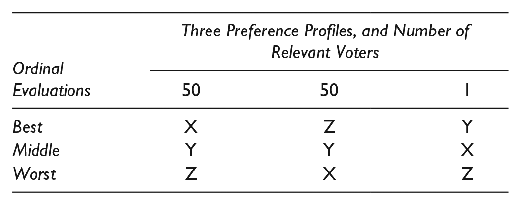
Given these preference profiles, candidate Y defeats X, 51 to 50, and also defeats Z, 51 to 50. Thus Y is the Condorcet winner—despite being the top choice of less than 1% of the voters.

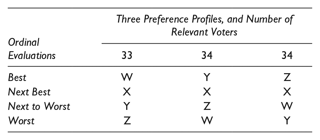
With four candidates the situation can be even more interesting. Suppose that our 101 voters are roughly evenly split into three groups, with their ordinal preferences as follows. Given this hypothetical division, candidate X is easily the Condorcet winner, overcoming each of the three opponents W, Y, and Z by large margins of roughly 2-to-1. Yet X is ranked first by absolutely no one (though second by everyone).¹⁶

Ordinal Evaluations	Three Preference Profiles, and Number of Relevant Voters
Ordinal Evaluations	33	34	34
Best	W	Y	Z
Next Best	X	X	X
Next to Worst	Y	Z	W
Worst	Z	W	Y

Data

The 2016 ANES had 4,271 respondents, of whom 1,181 were interviewed face-to-face and 3,090 via the Internet. Of the total, 3,649 answered both the pre- (9/7/16–11/7/16) and post-election (11/9/16–1/8/17) surveys; 622 completed only the former. In both the pre- and post-election surveys, respondents gave feeling-thermometer ratings (0°–100°) for each of four candidates: Hillary Clinton (Democrat), Donald Trump (Republican), Gary Johnson (Libertarian Party), and Jill Stein (Green Party).¹⁷ Most respondents rated Clinton and Trump, but failures to rate Johnson and Stein were common. In this section and later, we present only weighted results, with respondents weighted by their pre-¹⁸ or post-¹⁹election survey weights as appropriate.

Respondents who completed the post-election survey were classified as reported voters (RV) if they reported that they had voted.²⁰ All respondents, including those with no post-election survey, were checked through a voter validation procedure to see if they had actually voted and, if so, were classified as validated voters (VV).²¹ Some respondents, mainly some who did not do the post-election survey, were VV but not RV. Others, those who reported incorrectly that they had voted but apparently also some who really did vote but were counted as not validated because of imperfections in the validation procedure, were RV but not VV.

In this and later sections we show six sets of results, replicating the approach used by Abramson et al. (1995). They pertain to all respondents, RV, and VV for the pre-election survey, and likewise for the post-election survey. We label them as Pre All, Pre RV,²² Pre VV; Post All, Post RV, Post VV. These six sets correspond exactly to those used by Abramson et al. (1995) for 1980, as well as for 1968 and 1992 except that neither year had voter validations and 1968 had no feeling-thermometer ratings in the pre-election survey.

The six result categories reflect different conditions. Although pre-election feeling-thermometer ratings have the advantage of being uninfluenced by knowledge of the election results, post-election ratings may be based on fuller knowledge about the candidates, especially those who are lesser-known. Although elections obviously are decided only by those who vote, non-voters (especially those included in the Pre All and Post All sets) may be important if they might have become voters under different circumstances (e.g., more media exposure for lesser-known candidates, or a non-plurality election system that would reduce unease about “wasting” votes on such candidates).

Outcomes

Table 1 shows the details of the Condorcet analyses. We explain the table by using the fifth row of the Pre VV set for illustration. The (weighted) percentages of VV respondents who rated Trump higher than, equal to, and lower than Stein on the feeling thermometer in the pre-election survey are 39.59%, 6.04%, and 54.37%, respectively, which round to 40%, 6%, and 54%. These percentages are based on the 1803 VV respondents²³ who provided ratings for both Trump and Stein²⁴ in the pre-election survey. The “Difference %” value of −15.7%, though, is based only on those respondents—1698 out of the 1803—who gave Trump and Stein unequal ratings, and is calculated as (39.59% − 54.37%)/(39.59% + 54.37%). The two z-values, −5.46 and −5.51, test the statistical significance of the “Difference %” based on a normal approximation using two different modes of calculation²⁵ (which yield similar results both here and elsewhere in the table). The final two columns show the (weighted) average feeling-thermometer ratings, 36.8 for Trump and 41.6 for Stein, across all 1803 VV respondents who rated both candidates in the pre-election survey.

Table 1.

Condorcet Results: Weighted Percentage of Respondents Rating Each of Two Candidates Higher Than the Other, for Each of the Six Pairs of the Four Candidates in Each of the Six Respondent Sets.

Set^a	Candidate		% (weighted) for			N total	Difference %:(A>B)% − (A<B)% (A>B)% + (A<B)%	N for A>B and A<B	z-value for difference, by mode		Average rating (weighted)
Set^a	A	B	A>B	A = B	A<B	N total	Difference %:(A>B)% − (A<B)% (A>B)% + (A<B)%	N for A>B and A<B	1^b	2^b	A	B
Pre All	Clinton	Trump	51	7	42	4209	9.7	3939	5.04	4.23	42.0	36.7
	Clinton	Johnson	44	10	46	3209	−1.8	2891	−0.79	−0.75	42.0	43.4
	Clinton	Stein	45	12	43	2963	2.3	2628	0.97	0.89	42.7	42.5
	Trump	Johnson	36	9	56	3205	−21.8	2945	−9.92	−9.84	35.7	43.3
	Trump	Stein	37	7	55	2963	−19.3	2755	−8.49	−7.71	35.6	42.4
	Johnson	Stein	31	44	25	2784	9.7	1586	3.25	3.24	42.9	42.0
Pre RV	Clinton	Trump	52	5	43	2834	9.4	2709	4.06	3.64	42.9	36.6
	Clinton	Johnson	46	8	45	2213	0.8	2023	0.30	0.28	43.0	42.9
	Clinton	Stein	47	11	42	2022	5.6	1805	1.99	1.71	44.1	42.1
	Trump	Johnson	36	8	56	2214	−21.0	2061	−7.97	−7.78	35.5	42.9
	Trump	Stein	38	6	56	2025	−18.5	1909	−6.73	−6.17	35.3	42.0
	Johnson	Stein	32	41	26	1901	10.1	1121	2.83	2.90	42.3	41.6
Pre VV	Clinton	Trump	51	5	45	2544	6.1	2430	2.51	2.46	41.9	38.0
	Clinton	Johnson	45	8	47	1969	−1.8	1795	−0.62	−0.65	41.7	42.6
	Clinton	Stein	45	10	45	1800	0.7	1623	0.22	0.21	42.5	41.6
	Trump	Johnson	38	8	54	1970	−18.3	1826	−6.60	−7.09	37.0	42.5
	Trump	Stein	40	6	54	1803	−15.7	1698	−5.46	−5.51	36.8	41.6
	Johnson	Stein	33	42	26	1685	11.6	995	3.10	2.91	42.0	41.1
Post All	Clinton	Trump	48	6	46	3613	1.6	3409	0.75	0.64	43.9	42.3
	Clinton	Johnson	43	9	47	3004	−4.1	2741	−1.76	−1.64	43.7	44.4
	Clinton	Stein	44	12	44	3038	−0.1	2691	−0.06	−0.06	44.5	44.0
	Trump	Johnson	42	8	49	3012	−8.0	2765	−3.48	−3.46	41.4	44.4
	Trump	Stein	43	8	49	3044	−7.3	2828	−3.25	−2.86	41.3	44.0
	Johnson	Stein	34	35	31	2817	4.4	1822	1.58	1.59	44.1	43.9
Post RV	Clinton	Trump	49	4	47	2842	2.5	2733	1.06	0.98	44.3	42.5
	Clinton	Johnson	45	8	46	2419	−1.4	2232	−0.54	−0.51	44.5	43.5
	Clinton	Stein	46	11	43	2449	3.7	2180	1.44	1.35	45.2	43.0
	Trump	Johnson	43	8	49	2425	−6.0	2242	−2.33	−2.38	41.5	43.5
	Trump	Stein	44	7	49	2454	−6.0	2298	−2.37	−2.26	41.4	43.0
	Johnson	Stein	34	33	32	2279	2.6	1508	0.83	0.82	43.1	43.0
Post VV	Clinton	Trump	49	3	48	2239	0.9	2165	0.36	0.37	43.9	42.6
	Clinton	Johnson	45	8	47	1893	−2.6	1761	−0.92	−0.97	43.9	42.7
	Clinton	Stein	46	11	42	1911	4.2	1693	1.43	1.42	44.6	42.0
	Trump	Johnson	44	8	48	1898	−3.6	1758	−1.25	−1.38	41.9	42.8
	Trump	Stein	45	7	48	1915	−2.7	1791	−0.96	−0.94	41.96	42.03
	Johnson	Stein	34	34	32	1773	3.5	1154	0.99	1.00	42.5	41.9

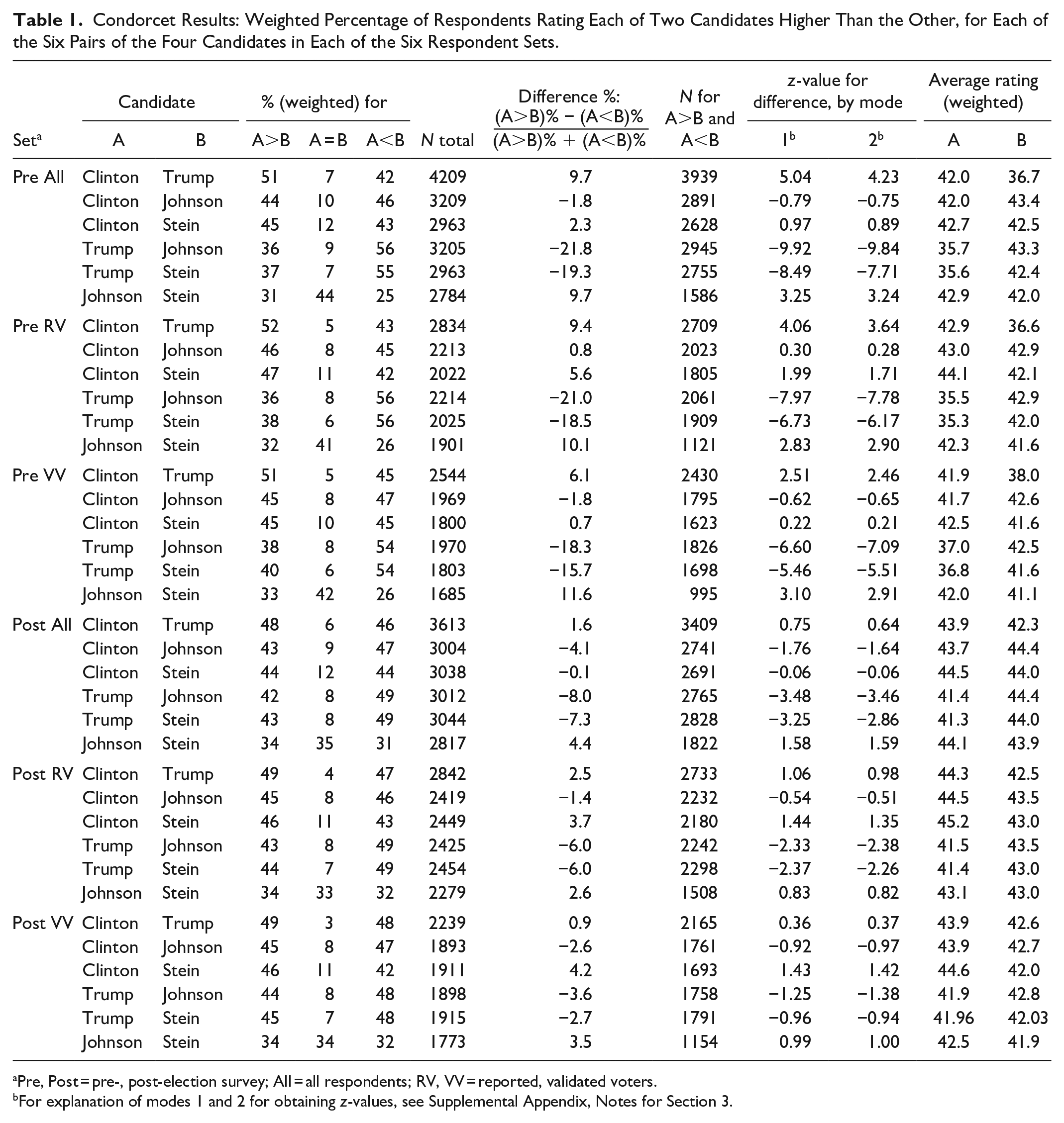
Pre, Post = pre-, post-election survey; All = all respondents; RV, VV = reported, validated voters.

For explanation of modes 1 and 2 for obtaining z-values, see Supplemental Appendix, Notes for Section 3.

Perhaps the strongest message from Table 1 is that, in all three of the pre-election sets, Trump loses heavily to each of his three opponents (perhaps surprisingly, even more to Johnson and Stein than to Clinton²⁶) and is thus the Condorcet loser. Statistical significance is far beyond the 0.01 level in eight of the nine comparisons (all except Clinton-Trump in the Pre VV set). Although Trump is also the Condorcet loser in each of the three post-election sets (by virtue of receiving fewer higher than lower ratings against each opponent), the “Difference %” is significant at the 0.05 level for only the Trump-Johnson and Trump-Stein comparisons in the Post All set and in the Post RV set.

The results for the three candidates other than Trump are less clear-cut. Johnson wins over Stein in all six sets, with statistical significance at the 0.01 level in the three pre-election sets but not even at the 0.05 level in the three post-election sets. Although almost all²⁷ of the Clinton-Johnson and Clinton-Stein comparisons lack significance at the 0.05 level, Johnson defeats Clinton in all sets except Pre RV and is thus the Condorcet winner in those five sets. Clinton is the Condorcet winner in the Pre RV set. She wins over Stein in all sets except Post All, where she barely loses to Stein and defeats only Trump.

We can recap with some rough conclusions covering the six result sets as a whole. It appears that a Condorcet loser was among the finalists in 2016; that may not be so unusual. The surprising thing is that the Condorcet loser was the Electoral College winner, Donald Trump.

This result is more decisive in the pre-election results, but it is universal in qualitative terms.

The Condorcet winner, if one existed,²⁸ could have been either Johnson or Clinton—not Stein—with the evidence slightly favoring Johnson, but not with anything approaching statistical significance. For further analysis of some matters concerning the Johnson-Clinton comparison and related issues, see Section 7 below.

The average ratings in the last two columns of Table 1 provide no surprises, given the conclusions already set forth. Of the 36 rows in the table, only three have a “Difference %” whose sign differs from the sign of the A-minus-B difference in average ratings. They are for Post All Clinton-Stein, Post RV Clinton-Johnson, and Post VV Clinton-Johnson, in all of which Clinton fares better on the rating difference than on the “Difference %.”

The results in Table 1 establish our primary conclusion: If there was a Condorcet winner in 2016, it was not Donald Trump. In fact, there is strong evidence that Trump was a Condorcet loser, in the sense that he would have lost a simple head-to-head popular-vote contest to literally any of the other candidates on the ballot: Clinton, Johnson, or Stein. Of course, it was already established empirically that Trump lost to Clinton in terms of actual popular vote, though it may be that filtering the results through the institution of the Electoral College influenced turnout.

That is why we try to use different methods to gauge likely voting outcomes.

Thus, it is worth asking what would have happened under alternative institutional scenarios. This more speculative analysis occupies us in the following section.

Use of Feeling-Thermometer Data to Project Results under Different Voting Systems

It is worth asking, to the extent that the data we possess can be used to make projections based on the feeling-thermometer ratings, how the 2016 election results could have turned out under various voting systems. Besides Condorcet, in this section we consider plurality voting, Borda, Hare, Coombs, range voting, and approval voting. Again, however, it is important to emphasize that the data may be substantially influenced by the fact that the strategies and time and resource allocations of campaigns were influenced by the institution of the Electoral College. To the extent that the patterns we observe are contingent on the strategies pursued, and that those strategies would have been different under the institutional systems we simulate, our conclusions are suspect. Besides, of course, we note again that the Electoral College is based on state vote totals, whereas our analyses use national results.

Further, we are assuming that voters would vote sincerely, in accord with their true preferences as inferred from the feeling-thermometer ratings. It could be argued that for plurality, Borda, and Coombs elections (at a minimum) this premise is untenable, and that strategic voting would have been extensive. Nonetheless, our resulting projections are still instructive, as the ANES respondents probably gave largely sincere ratings even if they did not vote sincerely.

To try to make projections that are as fair as possible and are comparable regarding both the seven systems and the four candidates, we take two preliminary steps before doing any of the basic analyses. First, for all seven systems, we exclude, separately for the three “Pre” sets and the three “Post” sets, those respondents who did not rate all four candidates in the pre- and post-election surveys, respectively.²⁹ Except for Condorcet, none of the systems can yield straightforwardly implied results without this exclusion.

Second, a respondent who gives two or three candidates the same rating causes complexity for some of the systems, because of tied ranks. To deal with this, we convert to untied ranks by replacing such a respondent with two, four, or six artificial respondents each carrying (respectively) 1⁄2, 1⁄4, or 1⁄6 of the original weight. Each resulting “respondent” has one of the 4! = 24 possible rankings of the candidates.³⁰ More simply, through assignment of (two, four, or six equally weighted) strong preference orders to an individual voter who has “tied” data, the numbers of votes received by tied candidates are correct in expected value (given equal probabilities in tie-breaking).

Table 2 shows the (weighted) percentage of (converted and unconverted) respondents having each of the 24 orderings. Note that four of these 24 rankings, those with Clinton at the top and Trump at the bottom or vice versa, account for about 60% or more of the total in each set. By contrast, the four rankings with Clinton first and Trump second or vice versa account for less than 7% of the total in each set.

Table 2.

For Each of the Six Sets, (Weighted) Percentage of Respondents Who Had Each of the 24 Possible Strict Rankings of the Four Candidates (After Respondents Having Tied Ratings Are Distributed to Appropriate Ones of the 24 Groups).^a

Ranking of				Percentage for^b
Clinton	Trump	Johnson	Stein	Pre All	Pre RV	Pre VV	Post All	Post RV	Post VV
1	2	3	4	1.3	1.5	1.4	1.8	1.8	1.7
1	2	4	3	1.6	1.7	1.1	1.7	1.7	1.5
1	3	2	4	1.4	1.4	1.2	1.7	1.7	1.6
1	3	4	2	1.9	1.9	1.9	2.2	2.4	2.3
1	4	2	3	16.3	16.9	16.7	13.8	14.1	13.8
1	4	3	2	17.8	19.0	18.8	17.9	19.8	20.3
2	1	3	4	2.2	1.8	1.6	1.9	1.6	1.7
2	1	4	3	1.8	1.4	1.4	1.6	1.3	1.2
2	3	1	4	0.4	0.3	0.3	0.5	0.3	0.2
2	3	4	1	0.6	0.6	0.6	0.5	0.5	0.5
2	4	1	3	3.1	2.9	2.5	1.8	1.6	1.5
2	4	3	1	3.0	2.7	2.6	3.3	3.1	2.7
3	1	2	4	2.8	3.0	2.9	4.1	4.5	5.1
3	1	4	2	1.9	2.0	2.3	1.6	1.6	1.6
3	2	1	4	0.7	0.6	0.5	0.8	0.7	0.8
3	2	4	1	0.4	0.3	0.3	0.7	0.7	0.5
3	4	1	2	4.8	4.2	4.2	2.9	2.5	2.3
3	4	2	1	3.9	3.1	3.0	3.9	3.1	2.8
4	1	2	3	14.0	14.6	15.9	17.1	17.7	18.1
4	1	3	2	10.8	11.1	11.8	11.5	12.0	12.9
4	2	1	3	2.3	2.2	2.4	2.4	2.3	2.4
4	2	3	1	0.9	0.6	0.6	1.4	1.4	1.1
4	3	1	2	3.7	3.8	3.8	2.8	2.2	2.0
4	3	2	1	2.6	2.3	2.2	2.2	1.6	1.4
Total				100	100	100	100	100	100
N total (number of respondents)				2718	1877	1661	2766	2250	1753

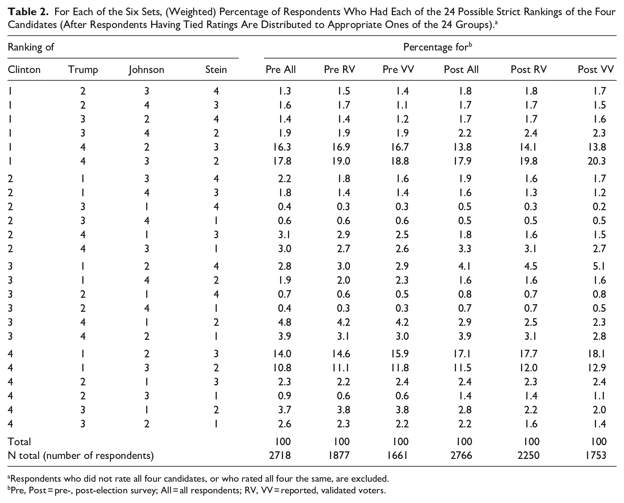
Respondents who did not rate all four candidates, or who rated all four the same, are excluded.

Pre, Post = pre-, post-election survey; All = all respondents; RV, VV = reported, validated voters.

The percentages in Table 2 were used to get the results for plurality, Hare, and Coombs but are not applicable for range voting or approval voting. Borda results can be found in two equivalent ways, one of them based on Table 2. The last row of Table 2 shows the number of (actual) respondents for each of the six sets (and applies to the calculations for all of the systems, including range voting and approval voting).

Condorcet Results, Using Only Respondents Who Rated All Four Candidates

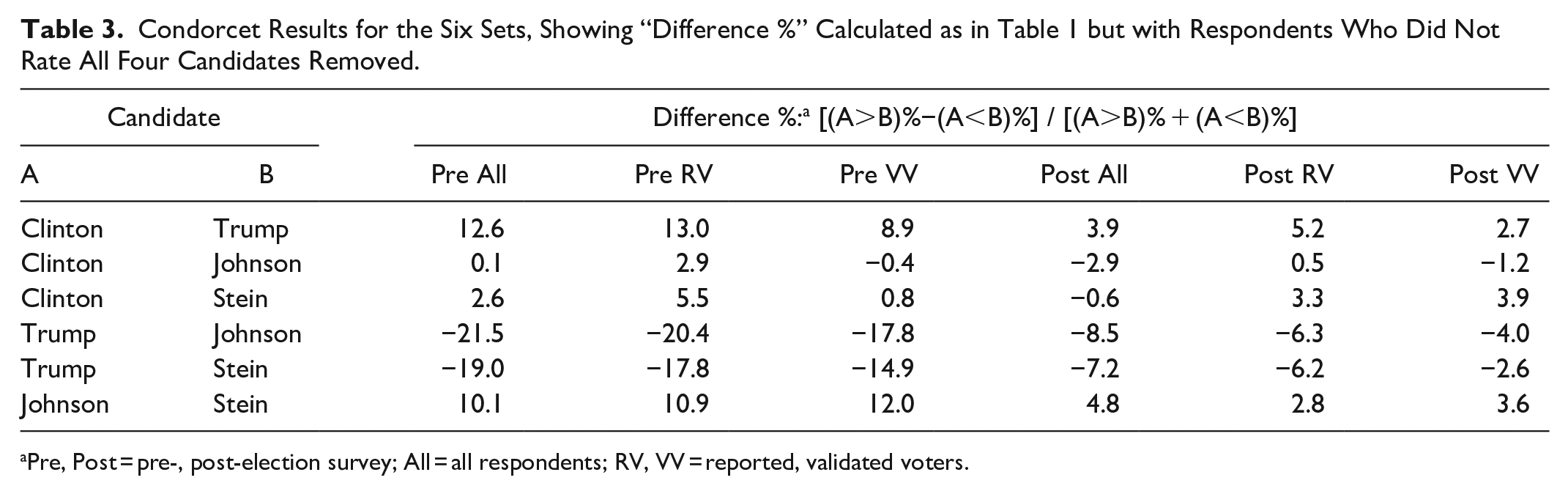
In order to have Condorcet results calculated for the same group of voters as those below for the other voting systems, we repeat the calculation of the “Difference %” that we did for Table 1 but exclude (for the Pre and Post sets separately) those respondents who did not rate all four candidates. In Table 3, “Difference %” has the same definition as before,³¹ but other information in Table 1 is omitted.

Table 3.

Condorcet Results for the Six Sets, Showing “Difference %” Calculated as in Table 1 but with Respondents Who Did Not Rate All Four Candidates Removed.

Candidate		Difference %:^a [(A>B)%−(A<B)%] / [(A>B)% + (A<B)%]
A	B	Pre All	Pre RV	Pre VV	Post All	Post RV	Post VV
Clinton	Trump	12.6	13.0	8.9	3.9	5.2	2.7
Clinton	Johnson	0.1	2.9	−0.4	−2.9	0.5	−1.2
Clinton	Stein	2.6	5.5	0.8	−0.6	3.3	3.9
Trump	Johnson	−21.5	−20.4	−17.8	−8.5	−6.3	−4.0
Trump	Stein	−19.0	−17.8	−14.9	−7.2	−6.2	−2.6
Johnson	Stein	10.1	10.9	12.0	4.8	2.8	3.6

Pre, Post = pre-, post-election survey; All = all respondents; RV, VV = reported, validated voters.

Of the 36 “Difference %” values, all but two have the same sign in Tables 1 and 3: In the Pre All and the Post RV sets, Johnson beats Clinton in Table 1 but loses in Table 3. More generally, Clinton fares noticeably better against both Trump and Johnson, but not Stein, in Table 3 than in Table 1—although otherwise the results in Tables 1 and 3 are closely similar. In particular, the more favorable results for Clinton against Johnson in Tables 3 versus 1 may imply at least some disadvantage for Johnson relative to Clinton in the results that follow below.

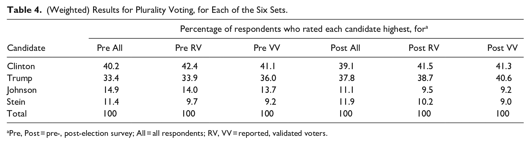
Plurality Voting

For each of the six sets, Table 4 shows the (weighted) percentage of respondents who rated each of the four candidates highest, calculated from the values in Table 2 (which take proper account of tied ratings). Thus, Table 4 shows the vote distribution under plurality voting, if everyone voted sincerely. Voters whose top choice is a minor-party candidate will often vote instead for a major-party candidate, however, rather than cast what may seem to be a “wasted” vote. In fact, the percentages for Johnson and Stein in Table 4 are far larger than their 2016 popular-vote percentages (which were 3.3% and 1.1%, respectively).

Table 4.

(Weighted) Results for Plurality Voting, for Each of the Six Sets.

Candidate	Percentage of respondents who rated each candidate highest, for^a
Candidate	Pre All	Pre RV	Pre VV	Post All	Post RV	Post VV
Clinton	40.2	42.4	41.1	39.1	41.5	41.3
Trump	33.4	33.9	36.0	37.8	38.7	40.6
Johnson	14.9	14.0	13.7	11.1	9.5	9.2
Stein	11.4	9.7	9.2	11.9	10.2	9.0
Total	100	100	100	100	100	100

Pre, Post = pre-, post-election survey; All = all respondents; RV, VV = reported, validated voters.

In all six sets in Table 4, Clinton is first and Trump is second. Stein noses out Johnson for third place in the Post All and Post RV sets, but Johnson beats her in the other four sets.

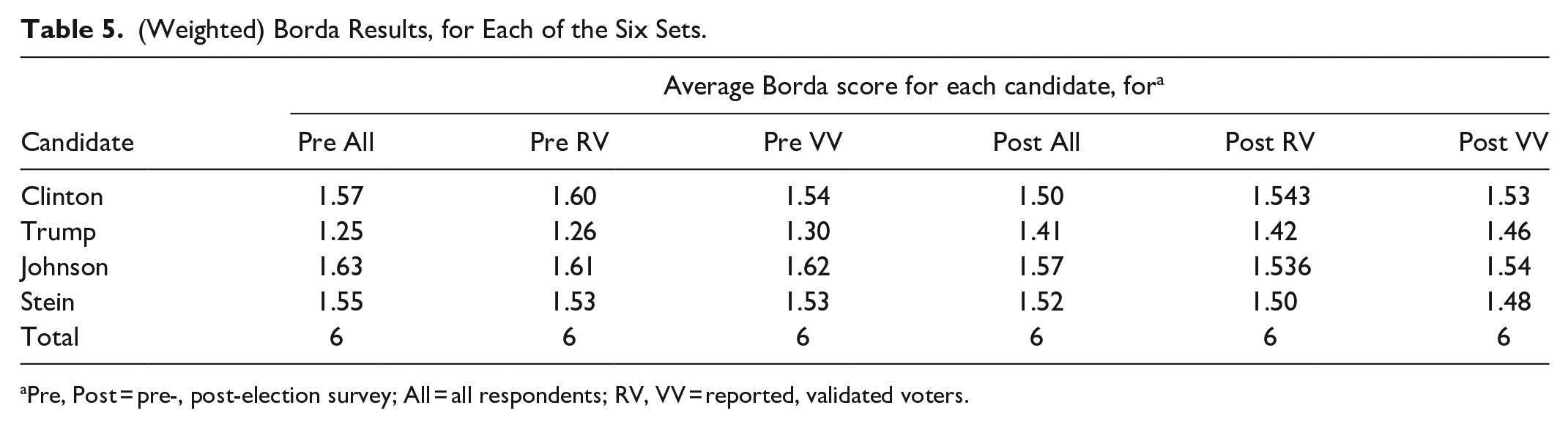
Borda

Table 5 shows the results for the Borda system. It is important to reemphasize that these results disregard strategic voting, to which the Borda system is vulnerable. Our claim is simply that ANES respondents would be unlikely to strategize when furnishing their candidate thermometer ratings anyway, and that our conclusions are supported by preferences even if they would not have been observed in empirical voting.

Table 5.

(Weighted) Borda Results, for Each of the Six Sets.

Candidate	Average Borda score for each candidate, for^a
Candidate	Pre All	Pre RV	Pre VV	Post All	Post RV	Post VV
Clinton	1.57	1.60	1.54	1.50	1.543	1.53
Trump	1.25	1.26	1.30	1.41	1.42	1.46
Johnson	1.63	1.61	1.62	1.57	1.536	1.54
Stein	1.55	1.53	1.53	1.52	1.50	1.48
Total	6	6	6	6	6	6

Pre, Post = pre-, post-election survey; All = all respondents; RV, VV = reported, validated voters.

The values in Table 5 can be calculated by giving scores of 3, 2, 1, and 0 to the candidates whom the respondent rates highest, second, third, and last, respectively (with the average of scores corresponding to tied ratings applied where such ties occur³²); and then weighting, summing, and dividing by the sum of the weights. Alternatively, the values can be found, in a similar manner, through use of Table 2. The two methods give the same results.

Trump is lowest in all six sets, and decisively so in the first three. Johnson is the Borda winner in all but the Post RV set, where Clinton barely beats him. Clinton is second in the remaining sets except for Post All, where she loses to Stein as well as Johnson. Stein is still a close third in the five sets besides Post All.

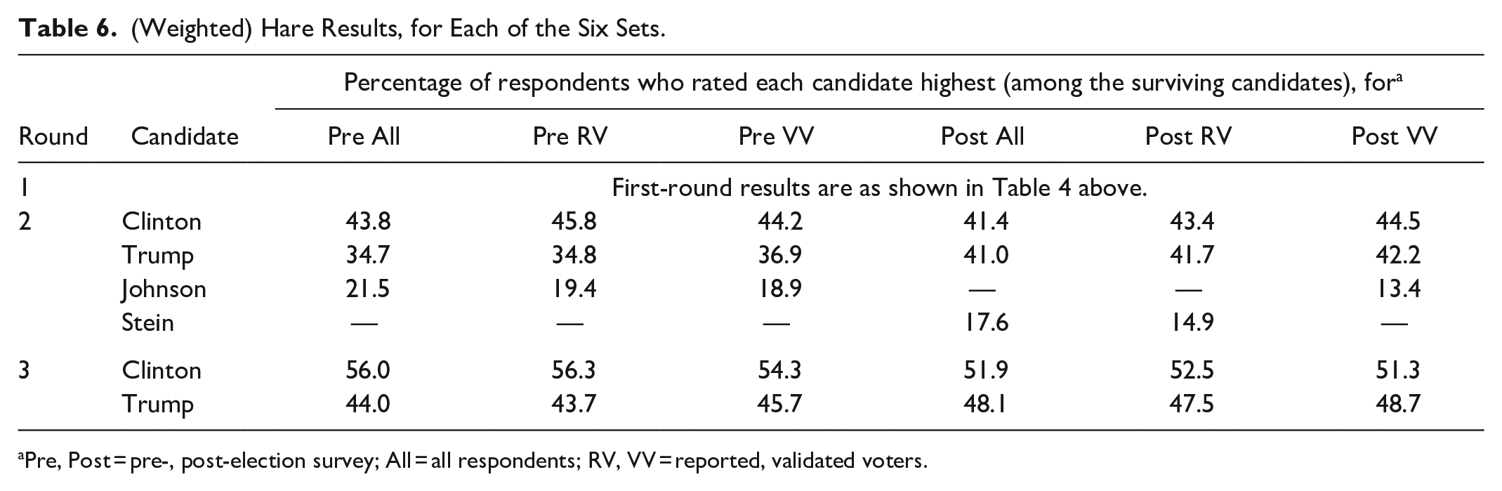
Hare

Table 6 shows the results for the Hare system (in its “single-winner” instantiation), also known as the alternative vote, “instant-runoff voting,” or “ranked-choice voting.” The system works in rounds or stages:

(1). Each voter ranks the candidates.

(2). On each round, the candidate who then has the fewest first-place votes is eliminated, and each ballot for the eliminated candidate is transferred to (and treated as a first-place vote for) the surviving candidate with the next highest ranking on that ballot.

(3). The next round proceeds with the modified rankings.

(4). The process ends when one candidate has a majority of the latest first-place votes.

Table 6.

(Weighted) Hare Results, for Each of the Six Sets.

Round	Candidate	Percentage of respondents who rated each candidate highest (among the surviving candidates), for^a
Round	Candidate	Pre All	Pre RV	Pre VV	Post All	Post RV	Post VV
1		First-round results are as shown in Table 4 above.
2	Clinton	43.8	45.8	44.2	41.4	43.4	44.5
	Trump	34.7	34.8	36.9	41.0	41.7	42.2
	Johnson	21.5	19.4	18.9	—	—	13.4
	Stein	—	—	—	17.6	14.9	—
3	Clinton	56.0	56.3	54.3	51.9	52.5	51.3
	Trump	44.0	43.7	45.7	48.1	47.5	48.7

Pre, Post = pre-, post-election survey; All = all respondents; RV, VV = reported, validated voters.

In Table 6, the first-round results are not shown, because they are identical to Table 4; the eliminated candidate is Johnson in the Post All and Post RV sets, and Stein in the other four sets. In the second round, Johnson and Stein are dropped in the respective sets where they survived.³³ The final round, in all six sets, pits Clinton against Trump with Clinton the winner.

Upon comparing the first round (Table 4) with the second round (Table 6), one discovers some interesting details. In each of the three Pre sets, more than half the votes of Stein (the removed candidate) transfer to Johnson. In the Post All and Post RV sets, about half or more of Johnson’s votes move to Stein. Almost half of Stein’s votes go to Johnson in the Post VV set.

Coombs

The Coombs system (Coombs, 1964, pp. 397–399; Grofman & Feld, 2004; Miller, 2014) is like the Hare system except that the candidate eliminated in each round is the one with the most last-place votes rather than the fewest first-place votes. In each round, the candidate with the most bottom-place votes is effectively removed from every ballot, after which the last-place votes for the surviving candidates are determined anew. There is one wrinkle: If any candidate has a majority of the first-place votes before an elimination is carried out, then that candidate is declared the winner. Thus, it is possible that a candidate with the most last-place votes also has a majority of the first-place votes; if that happens, that candidate is not eliminated, but rather is declared the winner.³⁴

The results for the Coombs system (Table 7) are intriguing. The following apply to all six sets. In round 1, Trump has by far the most last-place votes (and does not have a majority of first-place votes, per Table 4), so he is dropped. In round 2, Clinton now has easily the most bottom-place votes, so she is removed. (Even at this point, she has less than half the first-place votes, as can be determined by adding the seventh and eighth lines of Table 2 to the top line of Table 4). The final round matches Johnson against Stein, with Johnson winning.³⁵

Table 7.

(Weighted) Coombs Results, for Each of the Six Sets.

Round	Candidate	Percentage of respondents who rated each candidate lowest (among the surviving candidates), for^a
Round	Candidate	Pre All	Pre RV	Pre VV	Post All	Post RV	Post VV
1	Clinton	34.3	34.6	36.7	37.5	37.1	37.8
	Trump^b	48.8	48.8	47.8	43.6	44.2	43.5
	Johnson	8.1	8.0	7.5	8.2	8.2	7.5
	Stein	8.8	8.6	8.0	10.8	10.6	11.1
2	Clinton^b	43.0	41.9	43.9	44.2	42.7	43.0
	Johnson	28.9	29.7	28.8	29.4	31.1	30.6
	Stein	28.1	28.4	27.3	26.4	26.3	26.4
3	Johnson	47.1	46.8	46.5	48.4	49.0	48.8
3	Stein^b	52.9	53.2	53.5	51.6	51.0	51.2

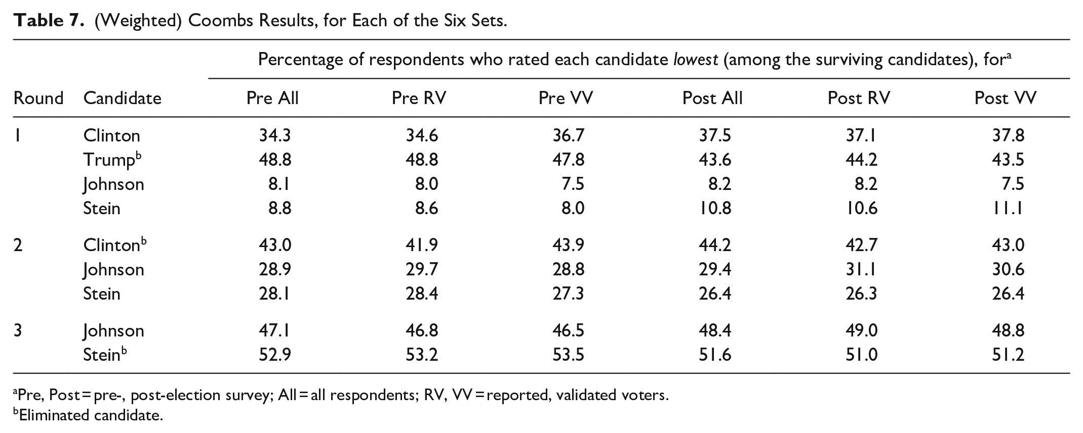
Pre, Post = pre-, post-election survey; All = all respondents; RV, VV = reported, validated voters.

Eliminated candidate.

Range Voting

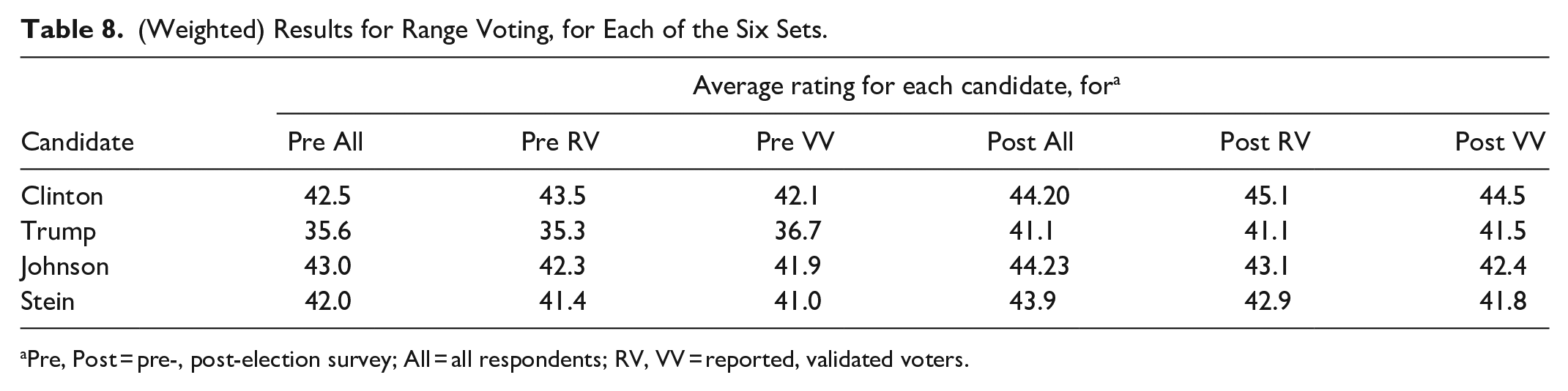
Long promoted by Warren D. Smith and advocated by Poundstone (2008, chapter 14), the range voting system has voters assign ratings—not ranks as in Borda, Hare, and Coombs—to each candidate.³⁶ The ratings are then totaled or averaged across all voters, and the highest-scoring candidate is the winner. We treat the ANES thermometer ratings (scale of 0º to 100º) as voter ratings for range voting, using them just as they are.

Table 8 gives the results for (weighted) average ratings for range voting. In all six sets, Trump is lowest (decisively so in the three Pre sets) and Stein is second lowest. Johnson barely edges out Clinton to win in the Pre All and Post All sets, but Clinton beats Johnson otherwise.

Table 8.

(Weighted) Results for Range Voting, for Each of the Six Sets.

Candidate	Average rating for each candidate, for^a
Candidate	Pre All	Pre RV	Pre VV	Post All	Post RV	Post VV
Clinton	42.5	43.5	42.1	44.20	45.1	44.5
Trump	35.6	35.3	36.7	41.1	41.1	41.5
Johnson	43.0	42.3	41.9	44.23	43.1	42.4
Stein	42.0	41.4	41.0	43.9	42.9	41.8

Pre, Post = pre-, post-election survey; All = all respondents; RV, VV = reported, validated voters.

Approval Voting

As was noted earlier, there appears to be at least a qualitative relationship between a Condorcet winner that no one dislikes “too much” and approval voting. Under approval voting (Brams & Fishburn, 2007), the voter votes for any number of the candidates on the ballot (though voting for none or all is ineffectual). The winner is the candidate who receives (approval) votes on the most ballots. (For one critique of approval voting, see Nagel, 2007).

Given that voting is sincere and not strategic, and given a voter’s rankings or ratings (where we are eliminating ties or indifference, by construction), there is, under all the voting systems we examined previously, only one way that the voter can mark the ballot. But that is not the case with approval voting, under which, with four candidates, the voter could sincerely vote for one, two, or three of them (compatible with the voter’s preference ranking). It is therefore requisite to define rules to specify how the ANES respondents would cast their approval votes given their feeling-thermometer ratings. This correspondence between preferences and how the ballot would be marked is arbitrary but possibly not innocuous, so we present three possibilities and calculate the results for each.

The central rules we employ for the correspondence between preferences and how the ballot would be marked are these:

(1). If the respondent gives equal (tied) ratings to candidates W, X, and Y and a lower rating to Z, then approval votes go to W, X, and Y.

(2). If the ratings for X, Y, and Z are equal and the rating for W is higher, then W alone receives an approval vote.

(3). If W and X are tied and also Y and Z are rated below them and tied with each other, then approval votes go to W and X.

(4). Otherwise, for the cases where the number of ties is zero or one, the rules for each scheme are as follows.

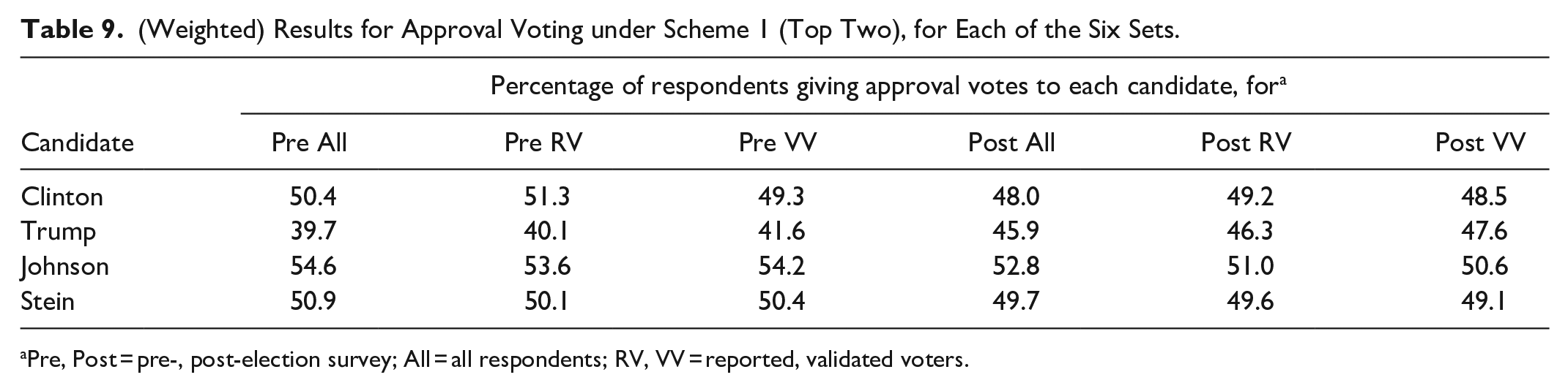
Scheme 1: Top two

If no ties exist, or if ties exist only between the highest two or lowest two ratings, then the candidates with the two highest ratings receive approval votes. If the ratings of candidates X and Y are tied but below W’s rating and above Z’s rating, then W receives an approval vote and X and Y each get half an approval vote.

Scheme 1 is in line with the result of Brams and Fishburn (2007, chapter 5) that a voter’s best strategy under approval voting is generally to vote for about half the candidates.

Chamberlin et al. (1984, p. 490) also use this principle in analyzing five annual elections of a professional society each with five candidates. Specifically, they examine two ways to ascribe approval votes: to (respectively) the top two and top three choices of each voter.

Table 9 shows the results for approval voting based on scheme 1. In all six sets, Johnson wins and Trump is at the bottom. For second place, Clinton tops Stein in the Pre RV set but loses to her in the other five.

Table 9.

(Weighted) Results for Approval Voting under Scheme 1 (Top Two), for Each of the Six Sets.

Candidate	Percentage of respondents giving approval votes to each candidate, for^a
Candidate	Pre All	Pre RV	Pre VV	Post All	Post RV	Post VV
Clinton	50.4	51.3	49.3	48.0	49.2	48.5
Trump	39.7	40.1	41.6	45.9	46.3	47.6
Johnson	54.6	53.6	54.2	52.8	51.0	50.6
Stein	50.9	50.1	50.4	49.7	49.6	49.1

Pre, Post = pre-, post-election survey; All = all respondents; RV, VV = reported, validated voters.

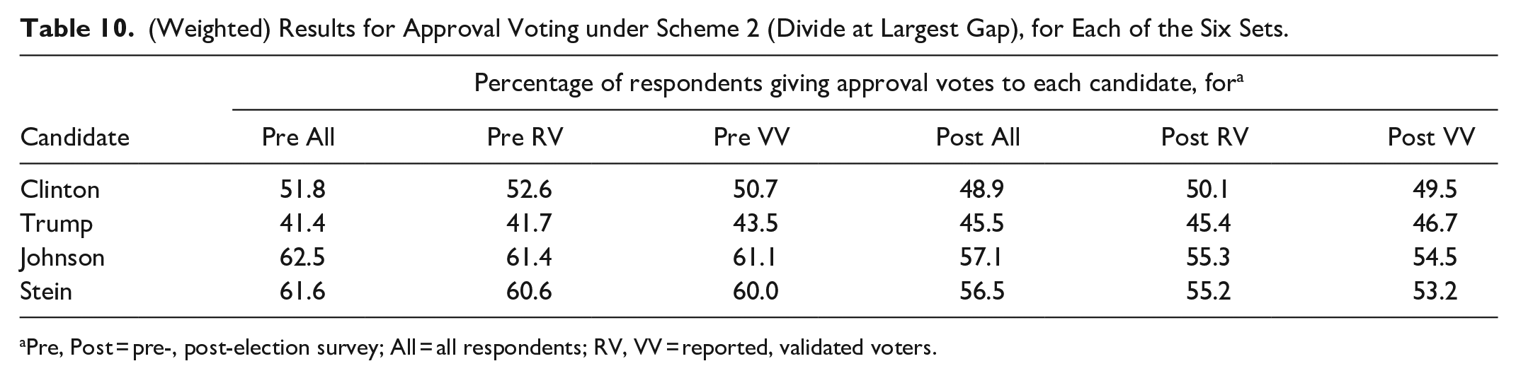
Scheme 2: Divide at largest gap

Let G1, G2, and G3 denote the respective differences between the top two, middle two, and bottom two ratings, with G1, G2, or G3 taken, respectively, to be 0 if the top two, middle two, or bottom two ratings are tied. If G1 > G2 and G1 > G3, then only the highest-rated candidate receives an approval vote. If G3 > G1 and G3 > G2, then an approval vote goes to each candidate except the lowest-rated one. Otherwise, the candidates with the two top ratings each receive an approval vote if G2 ≠ 0. If G2 = 0 and G1 = G3, the top-rated candidate gets an approval vote and the two (tied) middle-rated candidates are given half an approval vote each.

Scheme 2 and the gap criterion are reasonable and enjoy some precedent. Thus, for the 1968 U.S. presidential election, in one type of analysis of approval voting for a case where a voter gives thermometer ratings above 50° to all three candidates, Kiewiet (1979, p. 175 and Table II) ascribes an approval vote to a voter’s middle-rated candidate if and only if the ratings gap between middle and bottom ratings exceeds that between top and middle. Brams and Merrill (1994, p. 41, rule (1)) followed this same path in ascribing approval votes for the 1992 U.S. presidential election.

Results for approval voting with scheme 2 are in Table 10. In all six sets, Johnson wins, Stein is a close second, Clinton is third, and Trump is last. This happens to be the same ordering of the candidates as in Table 7, and almost the same as in Table 9.

Table 10.

(Weighted) Results for Approval Voting under Scheme 2 (Divide at Largest Gap), for Each of the Six Sets.

Candidate	Percentage of respondents giving approval votes to each candidate, for^a
Candidate	Pre All	Pre RV	Pre VV	Post All	Post RV	Post VV
Clinton	51.8	52.6	50.7	48.9	50.1	49.5
Trump	41.4	41.7	43.5	45.5	45.4	46.7
Johnson	62.5	61.4	61.1	57.1	55.3	54.5
Stein	61.6	60.6	60.0	56.5	55.2	53.2

Pre, Post = pre-, post-election survey; All = all respondents; RV, VV = reported, validated voters.

Scheme 3: Divide at rating of 50º

ANES respondents were instructed that candidate ratings between 50° and 100° indicate a favorable feeling toward the candidate and ratings between 0° and 50° mean that the respondent does not feel favorable. An ANES graphic labels a rating of 50° as "No feeling at all." It therefore seems appropriate to specify that a rating above, equal to, or below 50° for a candidate would correspond, respectively, to the respondent casting one approval vote, half an approval vote, or zero for that candidate. This is what is done for scheme 3, except that we provide for departures to ensure that each respondent gives a full approval vote to at least one of the four candidates and gives an approval vote of zero to at least one of them. Thus, if none of the four ratings is above 50°, we tally (full) approval vote(s) for the candidate(s) with the highest rating(s) (a tie can occur), and if no rating is below 50°, we tally approval vote(s) of zero for the candidate(s) with the lowest rating(s).

Since Scheme 3 is based on a division at 50° between favorable and unfavorable feelings, it may be the approach that conforms most closely to the basic concept of approval voting (which says that voters vote for those candidates they “approve of”). Methods like this also have prior usage (cf. Kiewiet, 1979, e.g.). Nonetheless, some concerns about scheme 3, peculiar to the 2016 data, can be raised, as we discuss in the Supplemental Appendix, Notes for Subsection 4.7.

Table 11 shows the results for approval voting under scheme 3. Johnson wins in the Pre All and Post All sets, but Clinton wins in the other four. Trump is last in all the sets except Post VV, where he is second and Johnson is fourth. Stein is second in two sets and third in four.

Table 11.

(Weighted) Results for Approval Voting under Scheme 3 (Divide at Rating of 50°), for Each of the Six Sets.

Candidate	Percentage of respondents giving approval votes to each candidate, for^a
Candidate	Pre All	Pre RV	Pre VV	Post All	Post RV	Post VV
Clinton	47.9	49.4	47.4	46.1	47.1	46.5
Trump	38.8	38.8	40.3	44.8	44.45	45.9
Johnson	48.6	46.8	46.2	47.4	44.46	42.3
Stein	47.1	45.4	43.5	47.2	45.0	42.9

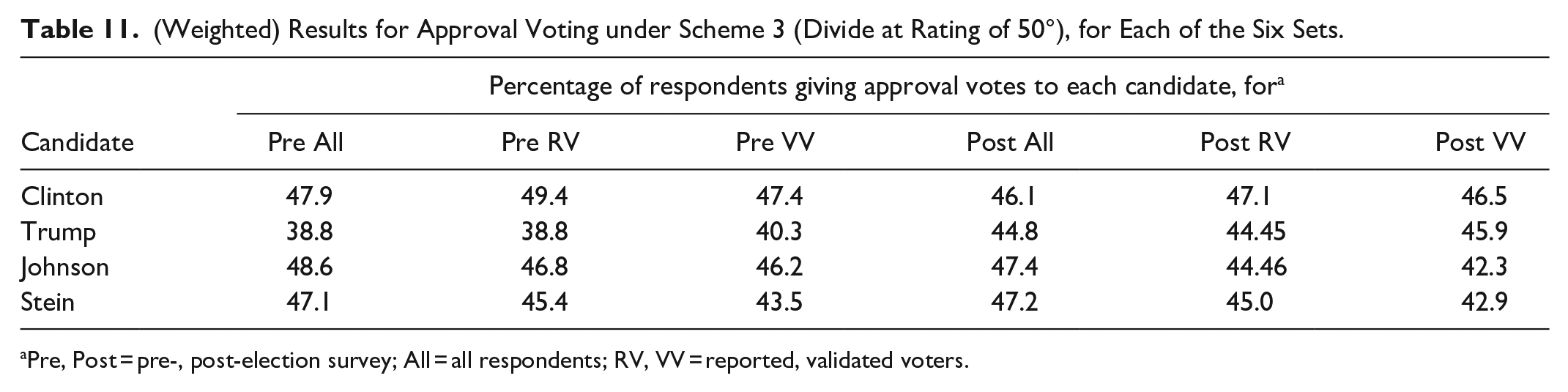
Pre, Post = pre-, post-election survey; All = all respondents; RV, VV = reported, validated voters.

As suggested earlier, results for approval voting are (highly) contingent on the correspondence rule. It is, of course, well-known that different rules for specifying (sincere) approval votes can lead to different results. Such inconsistency emerges in Tables 9 to 11 for schemes 1 to 3. Chamberlin et al. (1984, p. 488) also found such differences.

Summary for the Different Voting Systems

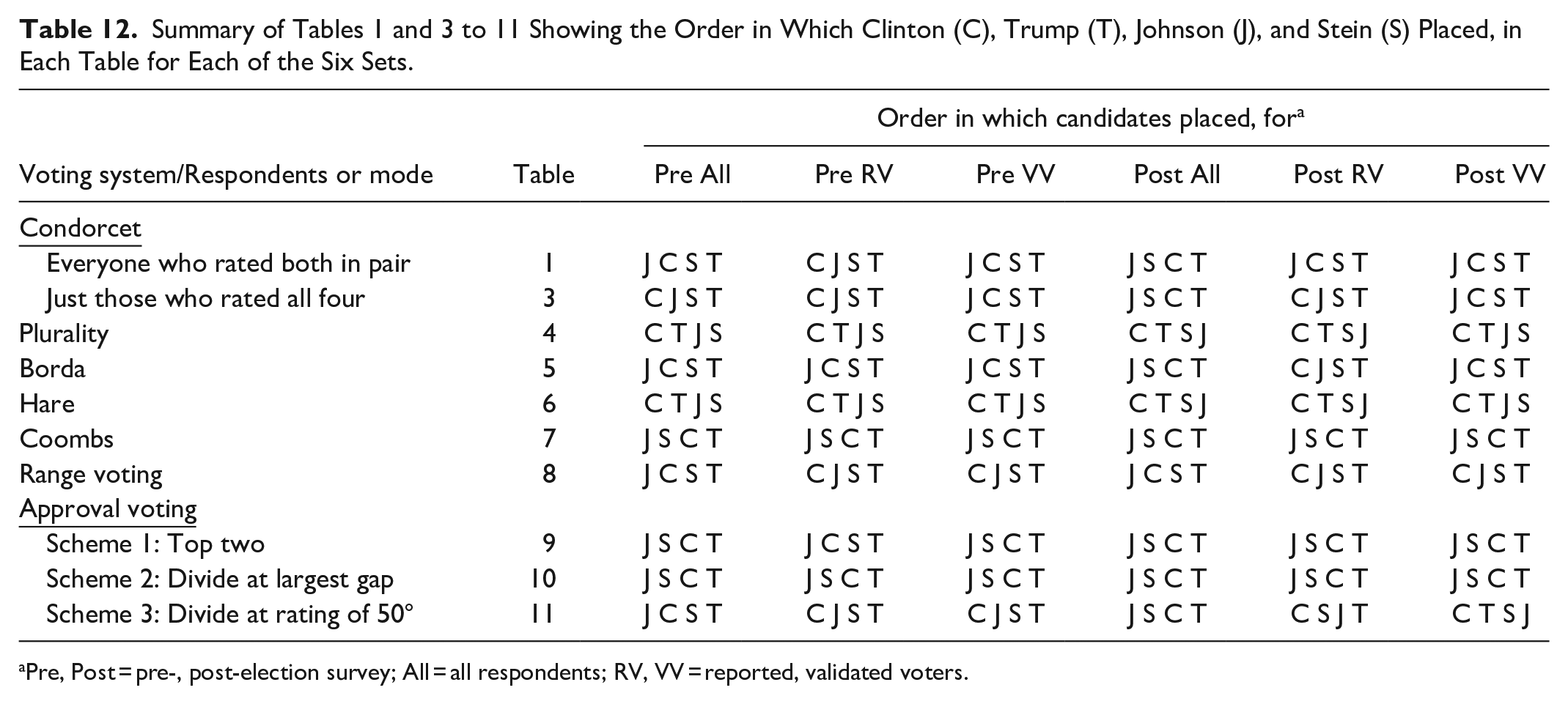
Table 12 summarizes the results for the seven voting systems and the six sets from Tables 1 and 3 to 11, by showing the order in which the four candidates place in each cell of the table. Metrics based on tallying the 60 cells in the table are quite crude but are nonetheless at least somewhat informative. Of the 60 first places, 35 go to Johnson and 25 to Clinton. Trump gets 47 of the last places, Stein 8, and Johnson 5. Though Trump and Stein have no first places, they have, respectively, 13 and 22 second places. Clinton has no last places but has 21 third places. Trump loses to Clinton in all 60 cells.

Table 12.

Summary of Tables 1 and 3 to 11 Showing the Order in Which Clinton (C), Trump (T), Johnson (J), and Stein (S) Placed, in Each Table for Each of the Six Sets.

Voting system/Respondents or mode	Table	Order in which candidates placed, for^a
Voting system/Respondents or mode	Table	Pre All	Pre RV	Pre VV	Post All	Post RV	Post VV
Condorcet
Everyone who rated both in pair	1	J C S T	C J S T	J C S T	J S C T	J C S T	J C S T
Just those who rated all four	3	C J S T	C J S T	J C S T	J S C T	C J S T	J C S T
Plurality	4	C T J S	C T J S	C T J S	C T S J	C T S J	C T J S
Borda	5	J C S T	J C S T	J C S T	J S C T	C J S T	J C S T
Hare	6	C T J S	C T J S	C T J S	C T S J	C T S J	C T J S
Coombs	7	J S C T	J S C T	J S C T	J S C T	J S C T	J S C T
Range voting	8	J C S T	C J S T	C J S T	J C S T	C J S T	C J S T
Approval voting
Scheme 1: Top two	9	J S C T	J C S T	J S C T	J S C T	J S C T	J S C T
Scheme 2: Divide at largest gap	10	J S C T	J S C T	J S C T	J S C T	J S C T	J S C T
Scheme 3: Divide at rating of 50°	11	J C S T	C J S T	C J S T	J S C T	C S J T	C T S J

Pre, Post = pre-, post-election survey; All = all respondents; RV, VV = reported, validated voters.

The voting systems appear to separate into three loose groups or categories of results. Borda and range voting follow Condorcet in mostly showing Johnson first and Clinton second or vice versa. Coombs and schemes 1 and 2 of approval voting have Johnson first and (except for one cell out of 18) Stein second. Plurality and Hare have Clinton first and Trump second in all cells, and (except for a single cell for scheme 3 of approval voting) are the only systems where Trump does not place uniformly last.

Are Preferences Single-Peaked? Who Are the Centrists?

Except under the plurality and Hare systems, our results above show surprising strength for Johnson and, to a lesser extent, for Stein. It is useful to look at factors related to, and reasons for, these results. We begin by examining the role of single-peaked preferences.

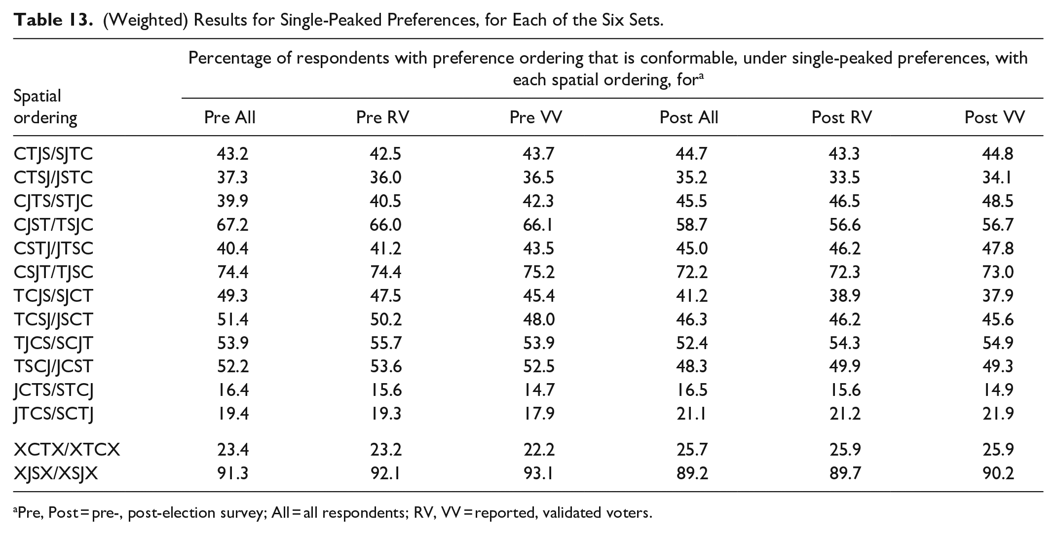
In a one-dimensional political space, Clinton (C) would generally be seen as to the left of Trump (T), and Stein (S) as to the left of Clinton. Johnson (J) would commonly, though not universally, be seen as to the right of Trump. Thus the ordering of the candidates, along this single dimension, would be SCTJ. Because the orientation is arbitrary, an equivalent spatial ordering, for purposes of determining single-peaked preferences, is the reverse, JTCS. The number of possible (non-equivalent) spatial orderings of the four candidates is 12, as shown in the first 12 rows of the first column of Table 13.

Table 13.

(Weighted) Results for Single-Peaked Preferences, for Each of the Six Sets.

Spatial ordering	Percentage of respondents with preference ordering that is conformable, under single-peaked preferences, with each spatial ordering, for^a
Spatial ordering	Pre All	Pre RV	Pre VV	Post All	Post RV	Post VV
CTJS/SJTC	43.2	42.5	43.7	44.7	43.3	44.8
CTSJ/JSTC	37.3	36.0	36.5	35.2	33.5	34.1
CJTS/STJC	39.9	40.5	42.3	45.5	46.5	48.5
CJST/TSJC	67.2	66.0	66.1	58.7	56.6	56.7
CSTJ/JTSC	40.4	41.2	43.5	45.0	46.2	47.8
CSJT/TJSC	74.4	74.4	75.2	72.2	72.3	73.0
TCJS/SJCT	49.3	47.5	45.4	41.2	38.9	37.9
TCSJ/JSCT	51.4	50.2	48.0	46.3	46.2	45.6
TJCS/SCJT	53.9	55.7	53.9	52.4	54.3	54.9
TSCJ/JCST	52.2	53.6	52.5	48.3	49.9	49.3
JCTS/STCJ	16.4	15.6	14.7	16.5	15.6	14.9
JTCS/SCTJ	19.4	19.3	17.9	21.1	21.2	21.9
XCTX/XTCX	23.4	23.2	22.2	25.7	25.9	25.9
XJSX/XSJX	91.3	92.1	93.1	89.2	89.7	90.2

Pre, Post = pre-, post-election survey; All = all respondents; RV, VV = reported, validated voters.

For present purposes we now use small letters, rather than capital letters, to designate the preference ordering determined from a respondent’s ratings of the four candidates.³⁷ Thus, an ordering of sctj means that the respondent rates Stein highest, Clinton second highest, Trump third, and Johnson lowest. (Note that the reverse ordering, jtcs, is not equivalent to sctj.) We use parentheses to denote tied ratings. Thus (e.g.) a respondent who rates Stein and Clinton each at 55 and Trump and Johnson each at 30 has the ordering (sc)(tj). There are 74 possible orderings of respondent ratings altogether: 4! = 24 with no ties, 36 with one two-way tie, six with two two-way ties, and eight with a three-way tie.

Consider, as an illustration, the spatial ordering JTCS/SCTJ. Of the 74 orderings of respondent ratings, 33 are conformable with single-peaked preferences under the spatial ordering JTCS/SCTJ;³⁸ the other 41 are not. The sum of the (weighted) percentages of respondents with the 33 respondent-rating orderings conformable under JTCS/SCTJ is 19.4% for the Pre All set, with similar values for the other five sets, as shown on the 12th line of Table 13.

The percentages for JTCS/SCTJ are by far the lowest in the table except for those on the 11th line (for JCTS/STCJ), which are lower. The respondents’ ratings are thus nowhere close to being in accord with a one-dimensional political space (with single-peaked preferences) that has Stein at one end, Johnson at the other end, and Clinton (next to Stein) and Trump (next to Johnson) in the middle.

Easily the highest percentages in the table are those for CSJT/TJSC, which are all above 70%. That spatial ordering has Clinton at one end, Trump at the other end, with Stein (next to Clinton) and Johnson (next to Trump) in the middle. The bottom two lines in Table 13 show the percentages of respondents who (given single-peaked preferences) have an ordering of their ratings that is conformable with one-dimensional spatial orderings that have, respectively, Clinton and Trump in the middle (spatial orderings of JCTS/STCJ and/or JTCS/SCTJ) and Johnson and Stein in the middle (spatial orderings of CJST/TSJC and/or CSJT/TJSC). The former percentages are around 25% or less. The latter are about 90% or more. Thus, based on this analysis, the centrists seem to be Johnson and Stein, not Clinton and Trump.

One might suspect this same type of result upon looking at or appropriately summarizing in Table 2. The calculations for Table 13 are more accurate, however, because for the purpose of single-peaked preferences they handle ties in a proper manner.

Principal Component Analysis

One may shed light from a different angle upon our off-key results by asking whether, for voters as opposed to legislators in the U.S., political space is actually unidimensional. The work of (e.g.) Poole and Rosenthal (2007) with roll-call data, based largely on their NOMINATE methodology, has found the U.S. Congress to be heavily polarized and (mostly) unidimensional, at least in recent times and especially in the most recent years. But, for the general public, the policy space may be more suitably defined by two or more dimensions, as recent studies by (e.g.) Carmines et al. (2012) and Feldman and Johnston (2014) attest. A multidimensional political space for voters could in some way produce enough of a jumble that it would be one factor affecting our results for 2016, as a space with more than one dimension can entail a complex preference structure. Since 2016 has some attributes of a “realigning” election (Azari & Masket, 2018), the question of dimensionality is particularly important.

To investigate the matter in a limited way, we chose 21 policy questions from the 2016 ANES, 11 from the pre- and 10 from the post-election surveys, and applied principal components analysis (PCA) to the sets of 21 answers from all 3,649 respondents who completed the post- as well as the pre-election questionnaire. This PCA made no use of the ratings data on the four presidential candidates. In an earlier use of PCA on political data, Potthoff (2018) applied it to the roll-call votes in the 1997-to-1998 and 1999-to-2000 U.S. Senates and found the respective percentages of total variability attributable to the first dimension to be 54.8 and 63.6, and the respective ratios of the second to the first eigenvalues to be 0.07 and 0.05.

Corresponding values for our PCA of the ANES policy questions show a much lower effect of the first dimension, and thus suggest greater dimensionality, or perhaps a fracturing of the shared understanding of the political space, for voters compared to legislators. The percentage of total variability accounted for by the first dimension is only 27.7, and the ratio of the second eigenvalue to the first is 0.29. Further detail concerning this PCA appears in the Supplemental Appendix, Notes for Section 6.

Assorted Results, Especially Ones That Affect the Clinton-Johnson Comparison

In the Supplemental Appendix, Notes for Section 7, are analyses for the following five points, which relate particularly to the Clinton-Johnson comparison but also are of broader interest:

Did ratings of candidates change during the two months before the 2016 election?

Did respondents who did and did not rate Johnson or Stein differ in their other ratings?

Did voters and non-voters rate candidates differently?

What can we tell about respondents who are excluded from Table 3 but not Table 1?

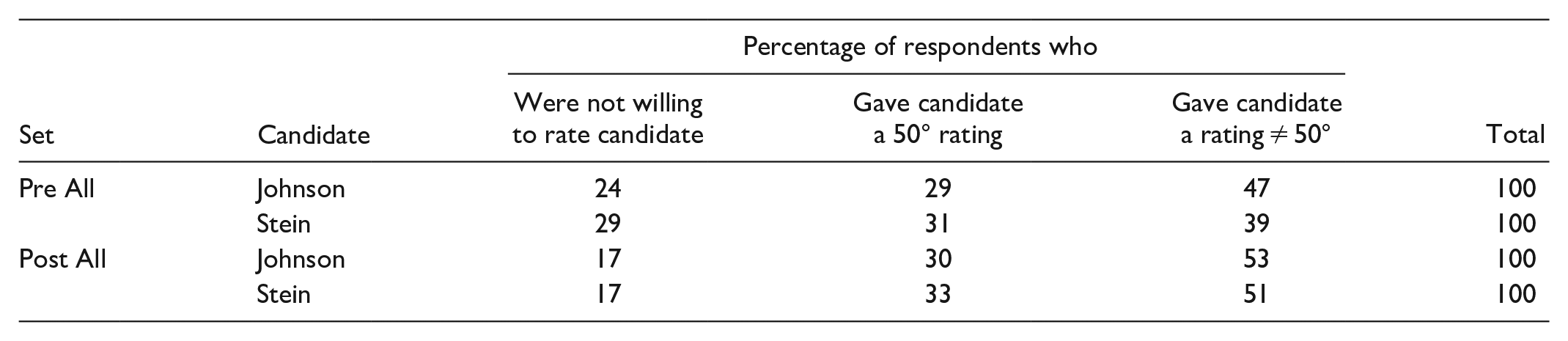
Johnson and Stein received many ratings of (exactly) 50º. What are the implications?

“Minor” Candidates and Thermometer Scores

In regard to item #5 just above, we first amplify by showing some specifics derived from the data in Table A6 in the Supplemental Appendix (see that table for more detail). For two (Pre All, Post All) of our six sets, and for each of Johnson and Stein, the following summary shows the (weighted) percentage of respondents who were not willing to rate them, who rated them at precisely 50°, and who rated them at other than 50°:

Set	Candidate	Percentage of respondents who			Total
Set	Candidate	Were not willing to rate candidate	Gave candidate a 50° rating	Gave candidate a rating ≠ 50°	Total
Pre All	Johnson	24	29	47	100
	Stein	29	31	39	100
Post All	Johnson	17	30	53	100
	Stein	17	33	51	100

Although item #5 receives extensive analyses in the Supplemental Appendix (Notes for Section 7, point 5), we provide below some general comments concerning thermometer ratings of both outsider and major-party candidates. (Regarding non-raters, see Notes for Section 7, point 2.)

We re-emphasize that our Condorcet findings in this paper relate to voters’ (sincere) preferences, not to votes themselves except that we do use the Condorcet results to project various votes assuming no strategic voting. Like earlier authors, we treat thermometer ratings as being sincere and not strategic, so that they can be used to deduce true preferences.

Although, unlike our analyses, Abramson et al. (1995) and Abramson et al. (2002) found no outsider candidate who was preferred to a major-party candidate, in many cases their outsider candidates still made respectable showings in two-way matchups against major candidates based on the thermometer ratings. In this sense, our results are not a radical departure from earlier ones. Still, one might wonder what factors could influence a thermometer-rating comparison between a major and a secondary candidate, and whether such factors could cause such a comparison to be murky perhaps because of extensive 50° ratings of the outsider. Relevant factors may include degree of polarization between the two major parties; whether the candidates, especially the outsiders, take extreme positions; extent of (good and bad) publicity received by an outsider; and (good or bad) personal qualities of all the candidates. Assessing the effects of these factors cannot be easy.

Polarization and negative partisanship (Bankert, 2020) were rampant in 2016. Trump and Clinton each received many ratings of 0° (see Table A10 in the Supplemental Appendix). Our results for range voting, and perhaps also for scheme 2 of approval voting, would have been less favorable to Johnson and Stein had the negative partisanship been less pronounced so that 0° ratings would have been replaced by values a little higher. To the extent that respondent rankings of the candidates would not have been altered by such replacement, however, our results for Condorcet and the other rank-based voting systems would not have changed.

One can ask whether (as we assume) a respondent who evaluates candidate X higher than Y on the thermometer scale would, in general, really vote for X over Y in a two-way (head-to-head, one-on-one) matchup. The approach has a long history in the literature (Aldrich et al., 2010; Endersby & Hinich, 1992; Rabinowitz, 1973), but in the current case we are considering a circumstance where X is an outsider with many 50° ratings and Y is a major-party candidate. If this approach is not justified, then presumably a different type of poll, one that asks directly about a (hypothetical) head-to-head vote, would show more respondents favoring Y over X than one based on thermometer ratings. We explore the issue in some detail in the Supplemental Appendix, Notes for Section 8, where we cite some head-to-head analyses. They include the 1980 ABC exit poll, mentioned earlier in footnote 12, which used head-to-head questions and showed Anderson (outsider candidate) over Carter whereas the thermometer ratings showed the reverse.

The notion that a candidate not from the two major parties could have meaningful support, or even be a Condorcet winner or almost be one, may be difficult to fathom. But a plurality voting system can obscure the viabilities of some such candidates.

Concluding Remarks

Using techniques applied by previous authors [including Abramson et al. (1995) and Abramson et al. (2002)] for earlier U.S. presidential elections, we used ANES pre- and post-election feeling-thermometer ratings to identify the Condorcet winner and the Condorcet loser among Clinton, Trump, Johnson, and Stein in the 2016 election. We found Trump to be the Condorcet loser, decisively so in the ANES pre-election survey. Whether Clinton or Johnson was the Condorcet winner is uncertain, though Johnson had a slight edge. In addition, Clinton has only a slim prevalence over Stein.

We offer briefly some final observations, opinions, and speculations:

Our results raise important questions about the artificial restriction of the presidential debates just before the general election to the two “major-party” candidates.

Media coverage that almost completely ignores “minor-party” candidates is likewise overly restrictive. Many voters might like to explore more than just two choices.

Traditional polls seek only vote intentions, not preferences. They cannot identify a Condorcet winner or loser. But the viability of candidates other than the two major ones can be assessed in part through Condorcet polling (e.g., Potthoff, 2011; Potthoff & Munger, 2015).

Citizens in robust democracies should understand what Condorcet winners and losers are, and should have confidence in the accuracy of voting procedures. At present, this lack of confidence is reaching crisis proportions, which suggests that education and media leadership could play a major role in ameliorating the problem.

Our results place Clinton and Trump at the extremes and Johnson and Stein in the middle. This may somehow partly reflect polarization of the two major parties, with each party’s base supporters hostile toward the other’s. But it could also indicate that the “minor parties” occupy a centrist position on a multidimensional mélange of many issues of liberty and government scope and conduct. We argue that the latter is a highly plausible explanation for the striking mix of the orderings that are most common and least common in Tables 2 and 13.

Table 12 and the tables that it summarizes exhibit surprising variation among the seven voting systems that we consider. The plurality system, currently predominant in the U.S. and elsewhere, suffers from vulnerability to strategic voting (especially from voters who want to avoid “wasting” their vote) and from the possibility³⁹ of failing to elect the Condorcet winner, or (worse, as we illustrate) electing the Condorcet loser. Replacing the plurality system would be desirable. That would seem unattainable over the short run, but maybe not over the long run.

Borda and Coombs would not be suitable substitutes because they are easily manipulated. Range voting may also invite appreciable strategic voting.⁴⁰ That leaves (single-winner) Hare, approval voting, and Condorcet.

Hare has made recent inroads by being adopted (see https://www.fairvote.org) in scattered jurisdictions in the U.S., including the state of Maine (in elections for U.S. House, U.S. Senate, and president), and has long been used in a few other places in the world. It has various weaknesses, though, as has been argued in the literature (Fishburn & Brams, 1983; Potthoff, 2013, Section 11).⁴¹ For statewide use in Maine, Maskin and Sen (2018) supported Hare, but apparently only, or largely, as a steppingstone toward a Condorcet system, which they prefer.

Where Hare is adopted, it would be beneficial to stipulate that the votes are tallied to identify not only the Hare winner but also (if one exists) the Condorcet winner. Useful information about differences between Hare and Condorcet winners would then be forthcoming.

Approval voting and Condorcet are leading alternatives to plurality. Approval voting—recently adopted for local elections in Fargo, North Dakota—need not elect the Condorcet winner but has the advantage of simplicity. A Condorcet system would, of course, need to specify a completion method, to be used in case no Condorcet winner emerges. Possible completion methods include those that revert to Borda (e.g., Black, 1958, p. 66), Hare (Green-Armytage et al., 2016), or approval voting (Nurmi, 1987, p. 176; Potthoff, 2013).

Finally, and perhaps most importantly, we would suggest that the use of Condorcet winners, and Condorcet losers, should be part of the evaluative tool kit for election rules. Schoolchildren are taught that elections are the way we choose the “best candidate.” But choosing a Condorcet winner, if one exists, and avoiding the selection of a Condorcet loser, if one exists, should be the way that “best” is fleshed out. The recent arguments claiming that the Electoral College should be replaced by a national “first past the post” plurality system do not solve this problem in any important way. By illustrating how different voting schemes incorporate these criteria, we hope to have advanced this discussion.

Supplemental Material

sj-pdf-1-apr-10.1177_1532673X211009499 – Supplemental material for Condorcet Loser in 2016: Apparently Trump; Condorcet Winner: Not Clinton?

Supplemental material, sj-pdf-1-apr-10.1177_1532673X211009499 for Condorcet Loser in 2016: Apparently Trump; Condorcet Winner: Not Clinton? by Richard F. Potthoff and Michael C. Munger in American Politics Research

Footnotes

Acknowledgements

The authors thank John Aldrich and two reviewers for their helpful comments. Errors and shortcomings that remain are likely the result of our inability fully to account for all the useful suggestions that were offered.

Declaration of Conflicting Interests

The author(s) declared no potential conflicts of interest with respect to the research, authorship, and/or publication of this article.

Funding

The author(s) received no financial support for the research, authorship, and/or publication of this article.

ORCID iDs

Richard F. Potthoff

Michael C. Munger

Supplemental Material

Supplemental material for this article is available online.

Notes

Author Biographies

Richard F. Potthoff is a mathematical statistician, is a Visiting Scholar in the Department of Political Science and the Social Science Research Institute at Duke University. Fields of publication include voting theory, elections, social choice, proportional representation, spatial models, design of election polls, prediction markets, linear and integer programming applications, biostatistics areas (design and analysis of clinical trials, missing data, case-control studies, genetics), and various areas of statistics (experimental design, multivariate analysis, homogeneity testing, regression, nonparametric statistics, latent-class models, psychometrics, telephone sample surveys).

Michael C. Munger is a political economist, is Professor in the Political Science Department, with courtesy appointments in the Economics Department and School of Public Policy at Duke University. Fields of publication include political institutions, regulatory policy, spatial models, and the new “sharing economy.” His most recent books have focused on problems of cronyism and the dramatic expansion of the commodification of excess capacity on new economic platforms.

References

Abramson

P. R.

Aldrich

J. H.

Paolino

Rohde

D. W.

(1995). Third-party and independent candidates in American politics: Wallace, Anderson, and Perot. Political Science Quarterly, 110(3), 349–367.

Abramson

P. R.

Aldrich

J. H.

Rohde

D. W.

(1998). Change and continuity in the 1996 elections. CQ Press.

Abramson

P. R.

Aldrich

J. H.

Rohde

D. W.

(2002). Change and continuity in the 2000 elections. CQ Press.

Abramson

P. R.

Aldrich

J. H.

Rohde

D. W.

(2006). Change and continuity in the 2004 elections. CQ Press.

Adams

Merrill

III Grofman

(2005). A unified theory of party competition: A cross-national analysis integrating spatial and behavioral factors. Cambridge University Press.

Aldrich

J. H.

Carson

J. L.

Gomez

B. T.

Rohde

D. W.

(2018). Change and continuity in the 2016 elections. Sage/CQ Press.

Aldrich

Dorobantu

Fernandez

(2010). The use of the left-right scale in individual’s voting decisions. Manuscript, presented at American Political Science Association.

Azari

Masket

(2018). Intraparty democracy and the 2016 election. In Lucas

J. C.

Galdieri

C. J.

Sisco

T. S.

(Eds.), Conventional wisdom, parties, and broken barriers in the 2016 election (pp. 137–162). Lexington Books.

Bankert

(2020). Negative and positive partisanship in the 2016 U.S. presidential elections. Political Behavior. https://doi.org/10.1007/s11109-020-09599-1

10.

Beinart

(2016, November 21). The Electoral College was meant to stop men like Trump from being president. Atlantic Monthly. https://www.theatlantic.com/politics/archive/2016/11/the-electoral-college-was-meant-to-stop-men-like-trump-from-being-president/508310/

11.

Black

(1958). Theory of committees and elections. Cambridge University Press.

12.

Blydenburgh

J. C.

(1988). Sophisticated voting in the 1980 presidential election. Political Behavior, 10(2), 103–116.

13.

Brams

S. J.

Fishburn

P. C.

(2007). Approval voting (2nd ed.). Springer.

14.

Brams

S. J.

Merrill

III (1994). Would Ross Perot have won the 1992 presidential election under approval voting? PS: Political Science & Politics, 27(1), 39–44.

15.

Buchanan

J. M.

(1954). Social choice, democracy, and free markets. Journal of Political Economy, 62(2), 114–123.

16.

Carmines

E. G.

Ensley

M. J.

Wagner

M. W.

(2012). Who fits the left-right divide? Partisan polarization in the American electorate. American Behavioral Scientist, 56(12), 1631–1653.

17.

Chamberlin

J. R.

Cohen

J. L.

Coombs

C. H.

(1984). Social choice observed: Five presidential elections of the American Psychological Association. The Journal of Politics, 46(2), 479–502.

18.

Coombs

C. H.

(1964). A theory of data. Wiley.

19.

Dasgupta

Maskin

(2004). The fairest vote of all. Scientific American, 290(3), 92–97.

20.

Endersby

Hinich

(1992). The stability of voter perceptions: A comparison of candidate positions across time using the spatial theory of voting. Mathematical and Computer Modeling, 16(9), 67–83.

21.

Feldman

Johnston

(2014). Understanding the determinants of political ideology: Implications of structural complexity. Political Psychology, 35(3), 337–358.

22.

Fishburn

P. C.

Brams

S. J.

(1983). Paradoxes of preferential voting. Mathematics Magazine, 56(4), 207–214.

23.

Forsythe

Myerson

R. B.

Rietz

T. A.

Weber

R. J.

(1993). An experiment on coordination in multi-candidate elections: The importance of polls and election histories. Social Choice and Welfare, 10(3), 223–247.

24.

Gehrlein

W. V.

(2006). Condorcet’s paradox. Springer.

25.

Gehrlein

W. V.

Lepelley

(2017). Elections, voting rules and paradoxical outcomes. Springer.

26.

Green-Armytage

Tideman

T. N.

Cosman

(2016). Statistical evaluation of voting rules. Social Choice and Welfare, 46(1), 183–212.

27.

Grofman

Feld

S. L.

(2004). If you like the alternative vote (a.k.a. the instant runoff), then you ought to know about the Coombs rule. Electoral Studies, 23(4), 641–659.

28.

Jones

J. M

. (2021, February 15). Support for third U.S. political party at high point. Gallup Politics. https://news.gallup.com/poll/329639/support-third-political-party-high-point.aspx

29.

Kiewiet

D. R.

(1979). Approval voting: the case of the 1968 election. Polity, 12(1), 170–181.

30.

Kurrild-Klitgaard

(2018). Trump, Condorcet and Borda: Voting paradoxes in the 2016 Republican presidential primaries. European Journal of Political Economy, 55, 29–35.

31.

Landemore

(2017). Beyond the fact of disagreement? The epistemic turn in deliberative democracy. Social Epistemology, 31(3), 277–295.

32.

Maskin

Sen

(2018, June 11). Maine tries a better way to vote. New York Times, p. A21.

33.

McLean

Hewitt

(1994). Condorcet: Foundations of social choice and political theory. Edward Elgar.

34.

Merrill

III (1988). Making multicandidate elections more democratic. Princeton University Press.

35.

Miller

N. R.

(2014). The alternative vote and Coombs rule versus first-past-the-post: A social choice analysis of simulated data based on English elections, 1992–2010. Public Choice, 158(3–4), 399–425.

36.

Muirhead

Rosenblum

N. L.

(2019). A lot of people are saying: The new conspiracism and the assault on democracy. Princeton University Press.

37.

Nagel

J. H.

(2007). The Burr dilemma in approval voting. The Journal of Politics, 69(1), 43–58.

38.

Nurmi

(1987). Comparing voting systems. Reidel.

39.

Poole

K. T.

Rosenthal

(2007). Ideology & Congress, second, revised edition of Congress: A political-economic history of roll call voting. Transaction Publishers.

40.

Potthoff

R. F.

(2011). Condorcet polling. Public Choice, 148(1–2), 67–86.

41.

Potthoff

R. F.

(2013). Simple manipulation-resistant voting systems designed to elect Condorcet candidates and suitable for large-scale public elections. Social Choice and Welfare, 40(1), 101–122.

42.

Potthoff

R. F.

(2018). Estimating ideal points from roll-call data: Explore principal components analysis, especially for more than one dimension? Social Sciences, 7(1), 12.

43.

Potthoff

R. F.

(2019). Three bizarre presidential-election scenarios: The perils of simplism. Social Sciences, 8(5), 134.

44.

Potthoff

R. F.

Munger

M. C.

(2005). Voter uncertainty can produce preferences with more than one peak, but not preference cycles: A clue to the fate of Ross Perot? The Journal of Politics, 67(2), 429–453.

45.

Potthoff

R. F.

Munger

M. C.

(2015). Condorcet polling can yield serendipitous clues about voter views. Public Choice, 165(1–2), 1–12.

46.

Poundstone

(2008). Gaming the vote: Why elections aren’t fair (and what can be done about it). Hill and Wang.

47.

Rabinowitz

G. B.

(1973). Spatial models of electoral choice: An empirical analysis. Institute for Research in Social Science, University of North Carolina at Chapel Hill.

48.

Regenwetter

Grofman

Marley

A. A. J.

Tsetlin

(2006). Behavioral social choice: Probabilistic models, statistical inference, and applications. Cambridge University Press.

49.

Reinhart

R. J.

(2020, February 13). Faith in elections in relatively short supply in U.S. Gallup Polls. https://news.gallup.com/poll/285608/faith-elections-relatively-short-supply.aspx

50.

Riker

W. H.

(1982). Liberalism against populism: A confrontation between the theory of democracy and the theory of social choice. W.H. Freeman and Company.

51.

Rothstein

(2018). Epistemic democracy and the quality of government. European Politics and Society, 20(1), 16–31.

52.

Rousseau

J. J.

(1973). The social contract (Trans. Cole

G. D. H.

). Dent.

53.

Schwartzberg

(2015). Epistemic democracy and its challenges. Annual Review of Political Science, 18(1), 187–203.

54.

Tabarrok

(2001). President Perot or fundamentals of voting theory illustrated with the 1992 election. Public Choice, 106(3–4), 275–297.

55.

Van Deemen

. (2014). On the empirical relevance of Condorcet’s paradox. Public Choice, 158(3–4), 311–330.

56.

Woon

Craig

Leifson

Tarpey

(2020). Trump is not a (Condorcet) loser! Primary voters’ preferences and the 2016 Republican presidential nomination. PS: Political Science & Politics, 53(3), 407–412.

Supplementary Material

Please find the following supplemental material available below.

For Open Access articles published under a Creative Commons License, all supplemental material carries the same license as the article it is associated with.

For non-Open Access articles published, all supplemental material carries a non-exclusive license, and permission requests for re-use of supplemental material or any part of supplemental material shall be sent directly to the copyright owner as specified in the copyright notice associated with the article.

0.00 MB

0.49 MB

Condorcet Loser in 2016: Apparently Trump;Condorcet Winner: Not Clinton?

Abstract

Keywords

Introduction

Background: The Normative Social Choice Problem

Condorcet Results

Overview and Examples

Data

Outcomes

Use of Feeling-Thermometer Data to Project Results under Different Voting Systems

Condorcet Results, Using Only Respondents Who Rated All Four Candidates

Plurality Voting

Borda

Hare

Coombs

Range Voting

Approval Voting

Scheme 1: Top two

Scheme 2: Divide at largest gap

Scheme 3: Divide at rating of 50º

Summary for the Different Voting Systems

Are Preferences Single-Peaked? Who Are the Centrists?

Principal Component Analysis

Assorted Results, Especially Ones That Affect the Clinton-Johnson Comparison

“Minor” Candidates and Thermometer Scores

Concluding Remarks

Supplemental Material

sj-pdf-1-apr-10.1177_1532673X211009499 – Supplemental material for Condorcet Loser in 2016: Apparently Trump; Condorcet Winner: Not Clinton?

Footnotes

Acknowledgements

Declaration of Conflicting Interests

Funding

ORCID iDs

Supplemental Material

Notes

Author Biographies

References

Supplementary Material