Sage Journals: Discover world-class research

Abstract

In this study, the fiber-shift method is presented to generate the three-dimensional geometric model of carbon fiber needled felt, and curved carbon fiber is regarded as beam under pure bending. The finite mixture model is applied to describe the fiber length distribution for the experiments and models. Closed model, open model and cut model are proposed, and cut model is thought to be more close to reality. A series of analytical methods are proposed to investigate the full-scale three-dimensional geometric model. The fiber-length distributions of cut models with different dimensions are obtained. The results show that, with the increasing of border length of cut model, the percentage of carbon fiber been cut is getting smaller, and the average fiber length is increased. In addition, the compression and needling process of pre-needling technique are simulated, and the needling hole obtained by simulation is similar to reality.

Keywords

Needled felt three-dimensional geometric model length distribution pre-needling process

Introduction

As versatile and cost-effective composites reinforcements, three dimensional (3D) needle-punched preforms have not only overcome the shortcomings of two-dimensional (2D) laminates [1,2] but also overcome the process complexity and high-cost disadvantage of other 3D preforms [3,4]. For 3D needle-punched composites, needled felt improved the interlaminar fracture toughness [5] and interlaminar shear strength [1], which was made primarily of high-performance fiber (carbon fiber, glass fiber, etc.). Fibers were cut into 40–100 mm, then carded and pre-needle-punched into needled felt. The interactions between fibers and carding elements were very complicated and often caused a considerable amount of fiber damages, so that, the length of different fibers was uncertain. In addition, the carbon fibers were randomly distributed, and they might be straight or curved.

Considerable attentions had been paid on the structure and properties of 3D needled composites or preforms [6,7], and the needled felt was always considered as isotropic material [2,8]. The morphology of needled felt has a deep impact on macroscopic properties, therefore detailed structural investigations are needed. The elastic modulus of needled felt reinforced composites can be obtained by the rule of mixtures, but the fiber length distribution is necessary [2,9,10]. Furthermore, the finite element model for needled felt reinforced composites needs 3D geometric models of needled felt. However, little knowledge about the internal structure parameters of carbon fiber needled felt had been reported, and there had been no attempt in realistically simulating the carbon fiber needled felt in a 3D geometry, which might be attributed to the complicated architecture of carbon fiber needled felt.

There are three families of methods for numerically generating random fiber assembly, namely the random sequential adsorption (RSA) schemes, random generation-growth (RGG) algorithm and image reconstruction technique [11]. The Monte Carlo (MC) procedure was always used to improve the fiber volume fraction. Based on these methods, many researchers generated representative volume element (RVE) of fiber reinforced composites, but the aspect ratio (the ratio of length to diameter) of random short fibers was only 1–200 [12 –14]. Besides, there were some 3D geometric models to simulate the diffusion of gas [15 –17], flow of fluids [18,19], transmission of heat and sound [14,20]. In these models, fibers were considered to be continuous and straight, so that, the aspect ratio was large enough in theory. However, the dimensions of these models were small. In fact, carbon fibers with different aspect ratio represent different behaviors in composites or preforms. The aspect ratio is in a range of 0–14000 in carbon fiber needled felt and it is thought that these models cannot reflect all the structure features. Pan et al. [11] proposed a modified RSA to generate an RVE of a short glass fibers web reinforced composite. In their model, RVE generation used both straight and curved fibers. In case of interpenetration, the new one had to bend away from the existing fiber to the sub-layer to avoid intersection. Nevertheless, the model appears not very realistic and the orientation distribution is restricted in-plane. In recent years, on the basis of 2D data from SEM images, Gaiselmann et al. [21–23] introduced a novel model that described non-interpenetrating fibers with strong curvatures and applied this model to simulate a non-woven gas diffusion layer consisting of carbon fibers. In this model, the length and shape of fibers was completely stochastic without considering the fiber properties. The modulus, orientation and length distribution will not affect the fiber model. To this end, the restrictions on the fiber structure are very low, and thus, these models are not suitable for carbon fiber needled felt, which is used for 3D needle-punched composites.

In this study, the statistical data are used to characterize the structure of carbon fiber needled felt. The curved carbon fiber is regarded as beam under pure bending and the fiber-shift method (FSM) is presented to generate the full-scale 3D geometric model of carbon fiber needled felt. Three kinds of full-scale 3D models are built, which are closed model, open model and cut model. The finite mixture model is applied to describe the fiber length distribution for the experiments and models. A series of analytical methods are proposed to investigate the full-scale 3D geometric model of carbon fiber needled felt. The fiber length distributions of cut models with different dimensions are obtained. The length distribution and average of fibers can be used to simulate the elastic modulus of carbon fiber needled felt reinforced composites. In addition, the compression and needling process of pre-needling technique are simulated.

Experimental

Materials

The Toray T300 carbon fibers were cut into 60 mm firstly. The fibers were fed into carding machine, and then pre-needling-punched into needled felt. The areal density of carbon fiber needled felt is 25 g/m². As a common raw material, the parameters for Toray T300 carbon fibers can be obtained by browsing the products catalogue and literatures, and the parameters are shown in Table 1. The needled felts were provided by Tianjin Polytechnic University.

Table 1.

The parameters of carbon fiber [24].

Parameter	Value
Longitudinal modulus (GPa)	230
Transverse modulus (GPa)	40
Longitudinal shear modulus (GPa)	24
Transverse shear modulus (GPa)	14.3
Tensile strength (MPa)	3530
Radius (µm)	3.5

Image analysis

In order to obtain plenty of statistical data, microphotographs are needed. Optical microscopes (ZEISS, Stemi 2000-C) and the SEM (HITACHI, TM1000) were used to observe the morphologies of fibers and needled felts. More than 400 microphotographs with different magnifications were obtained. Furthermore, the fiber orientations were measured by using image analysis technique on nonwovens fiber orientation analyzer (Donghua University, DHU-11).

Modelling

Finite mixture distributions

As a mathematical statistics modeling tool of analyzing a wide variety of random phenomena, finite mixture distributions can be used to define any complex probability distribution model [25]. If a set of data derived from an overall mixture and the overall distribution of the components is unknown, these data can be analyzed by means of the mixture model. A random variable x is said to have a finite mixture distribution if its probability density function (PDF) is of the form [26]

F (x) = \sum_{i = 1}^{k} λ_{i} f_{i} (x),

(1)

where F(x) is the PDF of the overall mixture and f_i(x) (1 ≤ i ≤ k) is the PDF of each component; k means the number of components, λ_i (1 ≤ i ≤ k) is the proportion of one component, which meets the prerequisite 0 ≤ λ_i ≤ 1, and

\sum_{i = 1}^{k} λ_{i} = 1

If each component submits to Weibull distribution, f(x) can be written as

f (x) = (γ_{i} / η_{i}) (x / η_{i})^{γ_{i} - 1} e^{- (x / η_{i}) γ_{i}}

(2)

where γ_i is the shape parameter and η_i is the scale parameter of the Weibull distribution.

For the characterization of carbon fiber length distribution, the mixture of two Weibull distributions has been used and the PDF can be expressed as

F (x) = λ (γ_{1} / η_{1}) (x / η_{1})^{γ_{1} - 1} e^{- (x / η_{1}) γ_{1}} + (1 - λ) (γ_{2} / η_{2}) (x / η_{2})^{γ_{2} - 1} e^{- (x / η_{2}) γ_{2}}

(3)

The fiber length distribution

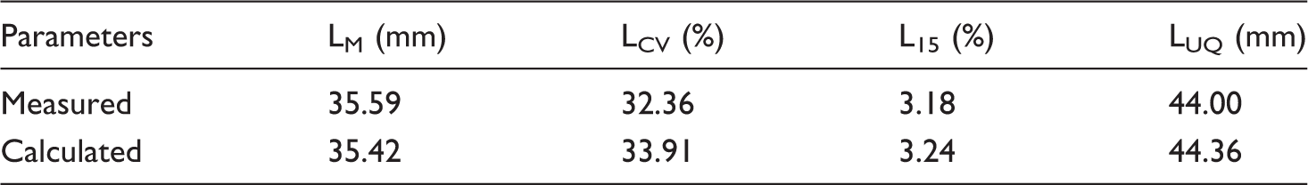
The fiber length is necessary for the 3D geometric model. In order to obtain real and effective data, 6000 fibers were measured. The fiber was pulled out from needled felt, which could not be cut off artificially, and then was measured. The software Weibull++10 was used to estimate the parameters of the mixture of Weibull distributions for histograms of fiber length distribution by the maximum likelihood estimation method. The fiber length distributions and the fitting curve are illustrated in Figure 1. To verify the PDF of the mixture Weibull distribution, some comparisons were carried out (Table 2). The detailed calculation methods are given by Kuang and Yu [25].

Figure 1.

The fiber length distribution of carbon fiber needled felt.

Table 2.

Comparison of the values obtained from the experiments and fitting curve.

Parameters	L_M (mm)	L_CV (%)	L₁₅ (%)	L_UQ (mm)
Measured	35.59	32.36	3.18	44.00
Calculated	35.42	33.91	3.24	44.36

L_M: the average fiber length; L_CV: the variable coefficient of fiber length; L₁₅: the content of fibers shorter than 15 mm; L_UQ: the upper quartile (75% percentile) of the statistical data.

In needled felt, carbon fibers may be straight or curved. The modulus of carbon fibers is large, so the bend cannot be seen until the fiber length is large enough. To obtain the minimum length of curved fibers, 2000 curved fibers were picked out and measured. Only 0.5% curved fibers in carbon fiber needled felt were shorter than 15 mm, so that, carbon fibers are considered to be straight if the fiber length is less than 15 mm. If not, carbon fibers should be straight or curved randomly. The length of the longest fiber was 60 mm, which was the original length before carding and pre-needle-punched. The smallest length was 6 mm. The aspect ratios of carbon fibers were from 850 to 8600. It is quite clear that carbon fiber needled felt is not a periodic-structure material. If the complete carbon fiber has to be shown, a full-scale 3D model is needed. Based on the statistical data, the fiber length list list_L had been built. Before a fiber is generated, the fiber length is selected in list_L randomly.

The bending parameters

Pure bending beam model.

In carbon fiber needled felt, the fiber suffers from complex forces, such as gravity, friction and squeeze. It is impossible to analyze the forces of each fiber accurately. It is known that, when beams are subject to equal and opposite bending moments M and M′ acting in the same longitudinal plane, such beams are said to be in pure bending [27]. The deformation of this beam is elastic. Because the deformation of carbon fiber before fracture is mainly elastic, it can be assumed here that the curved fibers can be treated as beams under pure bending. The bends of fibers were caused by manufacturing processes, and they were kept by gravities and interactions of fibers. In needled felt, single fiber might come into contact with a lot of fibers, and these fibers ‘held’ the single fiber to keep bending. In Figure 2(a), the curved fiber was ‘held’ by uncertain moments M_i, M_i₊₁…, M_m (i, m∈Z) and M_j, M_j₊₁…, M_n (j, n∈Z), and an uncertain part of fiber (l_c) did not suffer shear stress. The length and position of l_c were random, but they would be fixed when the force reaches a balance. Based on these discussions, it can be assumed as follows

The fiber is curved only in one longitudinal plane

$M = \sum_{k = i}^{m} M_{k}, M' = \sum_{k = j}^{n} M_{k}$ ;

$M = - M^{'}$

Figure 2.

Assumption of curved fibers: (a) The force distribution of fibers and (b) the fiber under pure bending.

M and M′ are acting on the left and right ends of the curved section l_c, respectively. As a result, l_c is under pure bending at this moment. According to the mechanics of materials

\frac{1}{ρ} = \frac{M}{EI}

(4)

where ρ is the radius of any point on l_c, E is the elastic modulus, I is the moment of inertia of the cross section with respect to a centroidal axis perpendicular to the plane of M, so that, ρ is constant and the shape of l_c is arc. In Figure 2(b), the fiber is composed of l_c, l₁ and l₂. l₁ and l₂ are tangent to l_c. The central angle and radius of l_c are α and r, respectively. In addition, for simplifying the single-fiber model, l₁ and l₂ are considered to be straight and it is assumed that only one arc part in a curved fiber. So the fiber length is

l = l_{1} + l_{c} + l_{2}

(5)

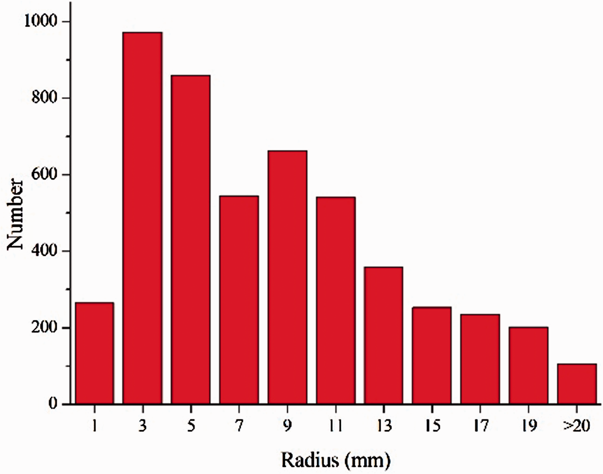
The distributions of radius of curvature of fiber.

In needled felt, the fibers are randomly distributed, which means that the location, the contact and the orientation of each fibers are different, so that, the stress conditions of different carbon fibers are different, and that results in the variation of bending parameters. According to the assumption of curved fiber under pure bending, it is necessary to input the bending parameters for the generation of model. The amplificatory picture of optical microscopes, magnified 6.5 to 20 times, were analyzed. It not only validated the assumption (Figure 3) but also measured the radius r. Three kinds of curved fibers were found in the microphotographs, they were curved fiber composed of one arc part and two straight parts (Figure 3b), curved fiber composed of one arc part (Figure 3c) and curved fiber composed of one arc part and one straight part (Figure 3d). For the last two, the fiber cannot be seen entirely in the microphotographs. Under the assumption that curved fiber is under pure bending, those fibers were also considered to be composed of one arc part and two straight parts, although some part of those fibers are not in the microphotographs. For obtaining sufficient data, 5000 numbers of radius were obtained, and the distributions are illustrated in Figure 4.

Figure 3.

The measurement of curved fibers: (a) The microphotographs of carbon fiber needled felt; (b) curved fiber composed of one arc part and two straight parts; (c) curved fiber composed of one arc part and (d) curved fiber composed of one arc part and one straight part.

Figure 4.

The distribution of radius of curvature of fiber.

The elongation at break of T300 carbon fiber is 1.5%. When the carbon fiber is under pure bending, the smallest radius before breaking can be calculated as follow

\frac{r α}{(r + \frac{D}{2}) α} = \frac{1}{1 + 1.5 %}

(6)

where D is fiber diameter, and the smallest radius before breaking is 0.23 mm. Similar results were obtained by other researchers [28]. In statistical data, the smallest radius was 1.31 mm, and that was considered to be reasonable. Furthermore, if the radius was larger than 20 mm, it was hard to measure, and this fiber was considered as a straight one, so that, the range of radius was from 1.3 mm to 20 mm in this model. The radius list list_R had been built on the basis of the statistical data of r. To avoid the interpenetration of two straight parts from one fiber, the upper limit of center angle α is π. When a single-fiber model for a curved fiber is generated, l is selected in list_L randomly, the radius is selected in list_R randomly. l_c is calculated from α and r, and α is randomly assigned.

The generation of single carbon fiber

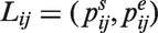
From the above, let F_i, i ∈ Z, be the single fiber, and it can be defined as

F_{i} = {L_{i 1}, L_{i 2}, \dots, L_{ij}}

where

L_{ij} = (p_{ij}^{s}, p_{ij}^{e})

is the jth line segment of the ith fiber consisting of starting points

p_{ij}^{s}

and ending points

p_{ij}^{e}

. For straight fibers, j = 1. It is convenient for calculating and analyzing by using this expression.

In this model, the fibers are considered to be randomly oriented in-plane. For a straight fiber with given l, the generation process based on FSM is shown in Figure 5(a). The p₁ (x₁, y₁, z₁) is set as starting point. Then assign a random numbers pair to the orientation angles (θ, ϕ) for each fiber to define the fiber orientation. It is easy to obtain the endpoint p₂ (x₂, y₂, z₂) by calculating from l, p₁ (x₁, y₁, z₁) and (θ, ϕ). The fiber is built on the generating line characterized by p₁ and p₂.

Figure 5.

Generation of single carbon fiber: (a) Straight fiber and (b) curved fiber.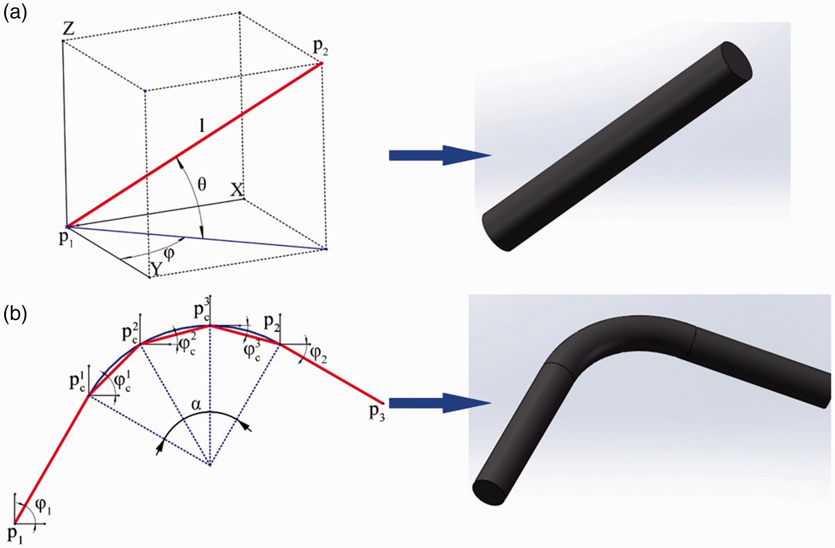

For a curved fiber, the single-fiber model is composed of one arc part and two straight parts. As Gaiselmann et al. [23] introduced, l_c is discretized into chains of small straight parts (Figure 5b). In this way, curved fibers can be simulated using a small number of parameters. Based on FSM, the curved fiber will be generated in 2D plane firstly. The p₁ (x₁, y₁) is set as starting point, and assign a random horizontal orientation ϕ₁ for the first straight part. With a given central angle α

{ϕ_{2} = ϕ_{1} - α ϕ_{c}^{k} = {ϕ_{1} - a / 2 m, k = 1 ϕ_{1} - a / 2 m - (k - 1) (a / 2 m), 1 < k << m

(7)

where m (m ≥ 1) is the number of straight parts. It is feasible to obtain the coordinates of

(p_{c}^{1}, p_{c}^{2}, p_{c}^{3}, p_{2}, p_{3})

by calculating from the length of each part, p₁ (x₁, y₁) and ϕ, and the fiber is built on the generating line characterized by

(p_{c}^{1}, p_{c}^{2}, p_{c}^{3}, p_{2}, p_{3})

The fiber-shift method

For RSA scheme and RGG algorithm, fibers are arranged in a region with arbitrary locations and orientations. They are not suitable for this model for two reasons. The first one is, the curved fiber is discretized into several straight parts, and the horizontal orientations ϕ of each part are related to each other. The other one is, the curved fiber is generated in one longitudinal plane, so the vertical orientation θ of each part is not random. Therefore, a new method is proposed, which is called FSM. By using this method, the single fiber is generated at the origin, then shifted to the appropriate position (Figure 6).

Figure 6.

Schematic of FSM: (a) Straight fiber and (b) curved fiber.

A box is defined to contain the fiber to be created, and the random displacement of this fiber in the box is defined as ( $Δ x, Δ y, Δ z$ ). The range of Δx, Δy, Δz can be calculated with the coordinate values of each straight part L_ij ( $p_{ij}^{s}$ , $p_{ij}^{e}$ ), to ensure the parts of fibers will not exceed the box limits. In addition, the new fiber is not accepted if it intersects fibers previously generated. If there is an interpenetration, a new random displacement is generated. This step keeps repeating until it is accepted. If the coordinate values of the point before shift is p^b (x^b, y^b, z^b), the coordinate values of the point after shift is p^a (x^a, y^a, z^a). It can be written as

{x^{a} = x^{b} + Δ x y^{a} = y^{b} + Δ y z^{a} = z^{b} + Δ z

(8)

For a curved fiber, the fiber is generated at the origin point in XY-plane. For clarity, a new plane is defined for the generation, which is called F-plane (Figure 7a). So, for all the points of each straight part, the z coordinate is zero. Assign three random angles (β_X, β_Y, β_Z) for the rotation. The range of β_X, β_Y, β_Z can be calculated with the coordinate values of the points, to ensure the parts of fibers will not exceed the box limits. Rotate the F-plane by β_X around X-axis (Figure 7b), by β_Z around Z-axis (Figure 7c), by β_Y around Y-axis (Figure 7d), respectively. If the coordinate values of the point before rotation is p^b (x^b, y^b, z^b), the coordinate values of the point after rotation is p^r (x^r, y^r, z^r). It can be written as

(x^{r}, y^{r}, z^{r}) = (x^{b}, y^{b}, z^{b}) [1000 \cos β_{X} \sin β_{X} 0 - \sin β_{X} \cos β_{X}] [\cos β_{Z} \sin β_{Z} 0 - \sin β_{Z} \cos β_{Z} 0001] \times [\cos β_{Y} 0 - \sin β_{Y} 010 \sin β_{Y} 0 \cos β_{Y}]

(9)

Figure 7.

The rotation of curved fiber: (a) Generation at the origin in XY-plane, (b) after rotation around X-axis, (c) after rotation around Z-axis and (d) after rotation around Y-axis.

After rotation, the fiber is shifted to the appropriate place with a random displacement ( $Δ x, Δ y, Δ z$ ). In this case, the curved fiber will be placed in arbitrary position in the defined box.

The avoidance of interpenetration

In this study, the interpenetration of fibers is not acceptable. As mentioned above, all the fibers are composed of one or several straight parts. It is easy to avoid the interpenetration by calculating the distance of straight parts in the box [29,30]. In order to reduce the computational burden, the box can be divided into several regions. It can be determined which region a new fiber was located, and the distance of straight parts only in this region can be calculated. In experiments, although the fiber bundles were found, most of the fibers were separated and not in fiber bundles. However, the collecting of fibers was influenced by the sizing and carding. The fiber bundles were neglected in this model. For carbon fiber needled felt, the sum of radius of two fibers is 7 µm. It is noted that once the fiber is generated, the shapes of fibers will not be changed. The avoidance of interpenetration is achieved only by the changes of location.

Full scale 3D geometry model

To generate the 3D geometric model, a Python script was developed based on Python 2.7.1. The script is executed in the commercial finite element software ABAQUS. Three kinds of models have been proposed, which are closed model, open model and cut model. The difference between closed model and open model is whether the entire fiber is limited in the box or not. For closed model, the generation and shift of fiber is carried out in the box strictly. No parts of fibers are not allowed to exceed the box limit. On the contrary, the fibers are allowed to generate out of the box for open model. In this case, the fiber is cut each time it goes through a face of box, retaining only the parts in the box. In addition, closed model will be cut around. The center region is left to be a smaller model, which is called cut model. These works are carried out by using Python script based on the coordinates of points of fibers.

Results and discussions

Closed model and open model

In 3D needle-punched preforms, the thickness of needled felt is about 0.1–2 mm. Based on these, the dimension of the model was 72 (length) × 72(width) × 2 (thickness) mm³. To compare with the sample, all the information of generated fibers were recorded in a specified recording file, such as l, r, θ, ϕ and so on. Two models were generated firstly and are illustrated in Figure 8. Only 1000 fibers were shown in each model for observing, but 2000 sets parameters of 2000 fibers were obtained by using Python script. The comparisons of real carbon fiber needled felt and the models were carried out in the following.

Figure 8.

The comparison of real carbon fiber needled felt and the models: (a) Closed model, (b) 12 × 12 mm² of closed model, (c) open model, (d) 12 × 12 mm² of open model, (e) the 3D view of closed mode, (f) arrangement of fibers and (g) 12 × 12 mm² of real carbon fiber needled felt.

The model in Figure 8(a) is named as closed model, and the other one is named as open model (Figure 8c). The fibers were composed of several straight cylinders without interpenetrating (Figure 8(f)), though it looked like lines. It is noted that, the number of fibers near the edge were less than the middle part in closed model. In order to avoid exceeding the box, it is easier to accept the fibers near the middle part. The reason for this is very complicated, which might include the length and number of fibers, the dimension of the box and the algorithm of generation. Any of them could conceivably influence the arrangement of fibers. However, what is interesting is this phenomenon also occurred in the actual production of needled felt [31].

To get accurate results, the model was divided into 36 regions. There were four kinds of regions, which were called corner region, border region, middle region and inner region. The starting point and ending point of each fiber in closed model and open model has been counted, and it can be determined where these points were located. It should be noted that, when the starting point or ending point was located on the model border of open model, it was ignored. That was because that point was created by cutting. The results are shown in Figure 9. It can be concluded that the number of starting and ending points is gradually increased from the edge to the inside of closed model. However, the number of starting and ending points in each area is basically the same in open model, which means the fibers are evenly distributed.

Figure 9.

The number of starting and ending points of closed model and open model.

Other parameters of experiment and the models are compared in Figures 10 and 11. All the data were calculated from coordinates of points of fibers by using Python script. It is important that, only the orientation angles of straight parts of fibers in the model were recorded, so the discrete arc parts were not included in the calculations. For straight fiber, one orientation angle was recorded, and there were two for curved fibers. In addition, the radius was only for curved fibers. As shown in Figure 10, this modeling approach offers a nice control of the orientation and radius of curvature of fiber. That is because the orientation angle was randomly assigned from –π to π, and the radius of curvature of fiber was randomly selected from the list of statistical data. Although fibers were arranged evenly in open model, the fiber length distributions of open model were different from that of experiments (Figure 11). For open model, the length value was randomly selected in the list of statistical data, but the fibers were cut when they exceeded the box for open model. That resulted in the change of length distribution, and there were more shorter fibers and less longer fibers in open model. The average length (27.32 mm) was less than experiment (35.59 mm) and closed model (35.58 mm). More fibers were generated to study the influence of number of fibers for open model. The results showed that (Figure 11c), the number of shorter fibers increased with the increase of number of fibers in open models. This problem will be solved by using periodic boundary conditions [32,33], but that is not suitable for this model.

Figure 10.

The parameters of experiment and the models: (a) Fiber orientation distribution and (b) curvature radius distribution.

Figure 11.

The length distribution of experiment and the models: (a) The comparison of experiments and closed models, (b) the comparison of experiments and open models and (c) the comparison of different numbers of fiber for open model.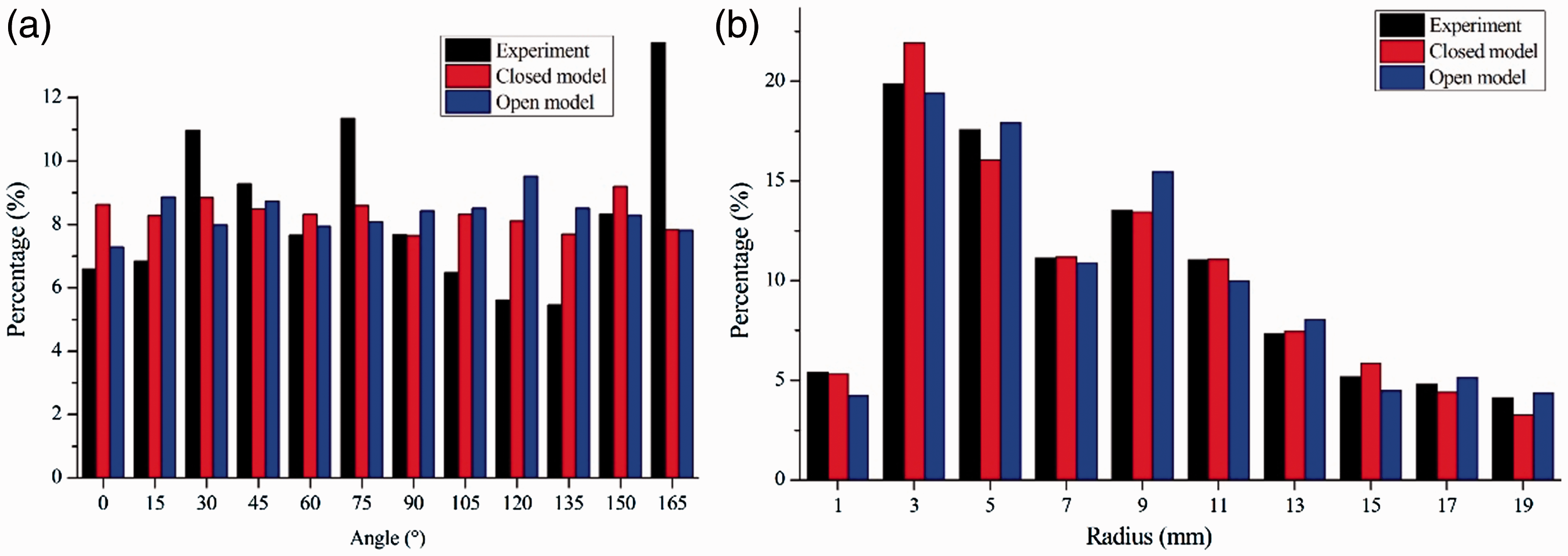

Cut model

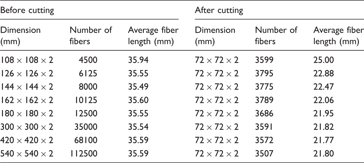
In experiment, the fibers were not cut off artificially. The closed model is a simulation of a whole needled felt without any cut. However, almost all of the needled felts have been cut in the applications, and the uneven selvedge should be removed during the manufacturing process. In order to build more realistic model, eight bigger boxes were used to generate closed models of carbon fiber needled felt, then they were cut into cut models. For the sake of contrastive analysis, the ratio of number of fibers to volume of box was equal for each closed model. The information of closed models is listed in Table 3, and Figure 12 shows the schematic of some cutting models.

Table 3.

The parameters of closed models.

Before cutting			After cutting
Dimension (mm)	Number of fibers	Average fiber length (mm)	Dimension (mm)	Number of fibers	Average fiber length (mm)
108 × 108 × 2	4500	35.94	72 × 72 × 2	3599	25.00
126 × 126 × 2	6125	35.55	72 × 72 × 2	3795	22.88
144 × 144 × 2	8000	35.49	72 × 72 × 2	3775	22.47
162 × 162 × 2	10125	35.60	72 × 72 × 2	3789	22.06
180 × 180 × 2	12500	35.55	72 × 72 × 2	3686	21.95
300 × 300 × 2	35000	35.54	72 × 72 × 2	3591	21.82
420 × 420 × 2	68100	35.59	72 × 72 × 2	3572	21.77
540 × 540 × 2	112500	35.59	72 × 72 × 2	3507	21.80

Figure 12.

The schematic of cutting closed models: (a) 108 × 108 × 2 mm³, (b) model cut from 108 × 108 × 2 mm³, (c) 126 × 126 × 2 mm³, (d) model cut from 126 × 126 × 2 mm³, (e) 144 × 144 × 2 mm³, (f) model cut from 144 × 144 × 2 mm³, (g) 162 × 162 × 2 mm³, (h) model cut from 162 × 162 × 2 mm³, (i) 180 × 180 × 2 mm³ and (j) model cut from 180 × 180 × 2 mm³.

The model cut from a bigger closed model is named as cut model. Unlike open model, the cut model is built based on closed model. As the most important parameter for property, the length distribution was investigated by using the mixture of two Weibull distributions. When the total fiber length of each model is about 0.6 × 10⁵mm, the fiber length distributions of each cut models are illustrated in Figure 13. It can be seen that, the length distributions of cut models are different. The average fiber length decreases with the increase of closed model dimension, until the border length (the edge length in XY-plane of the model) of the model reaches 162 mm.

Figure 13.

The fiber length distributions of cut models.

It is easy to understand that the in-plane property of needled felts will be affected by the average fiber length, unless the dimension of needled felt is large enough. It is thought that, the cut model is more close to the practical application of needled felt, so that, it is important to obtain the length distributions of cut models with different dimensions, which will provide basis for the simulation of mechanical properties in-plane of carbon fiber needled felt. For this reason, three biggest models were cut into several small cut models. In order to further analyze these cut models, the percentage of fiber been cut is illustrated in Figure 14(a), and the average fiber length of these cut models is illustrated in Figure 14(b).

Figure 14.

The relationship between the border length of cut model and fiber length: (a) Percentage of fiber been cut and (b) average fiber length in each cut model.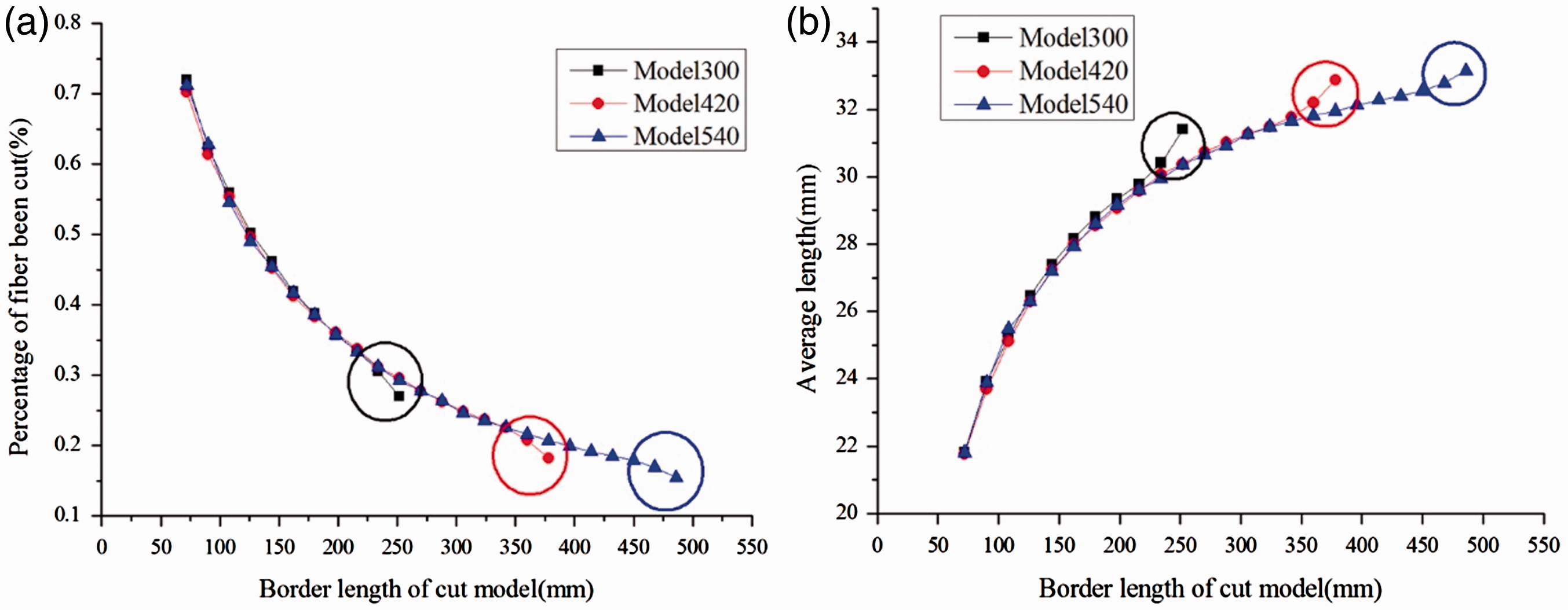

It can be seen that, with the increasing of border length of cut model, the percentage of fiber been cut is getting smaller, and the average fiber length is increased. The curves of three closed models have good coherence to each other. It is important to note that, for Model300, when the border length of cut model is bigger than 234 mm (marked by black circle), the data begin to fluctuate. For Model420, when the border length of cut model is bigger than 360 mm (marked by red circle), the data begin to fluctuate. For Model540, when the border length of cut model is bigger than 486 mm (marked by blue circle), the data begin to fluctuate. We have mentioned above that there are less fibers near the border of closed model. When the dimension of cut model is close to the closed model, the number of fiber been cut decreases sharply, and the average fiber length increases significantly. It is believed that, for Model300, if the border length of cut model is no more than 216 mm, the length distributions and average fiber length are stable and valuable. For Model420, the border length of cut model is no more than 342 mm; for Model540, the border length of cut model is no more than 468 mm. Based on these length data, if the border lengths of closed model are defined as a function of the border length of cut model L_b

f (L_{b}) = (L_{b} + 99) / 1.05

(10)

When the border length of cut model is 72 mm, the border length of closed model calculated from formula (9) is 162.86 mm, which is consistent with the previous results.

In conclusion, a series of analytical methods were proposed to investigate the full-scale 3D geometric model of carbon fiber needled felt. From these discussions, if the length distribution or the average fiber length in carbon fiber needled felt with certain dimension is needed, a bigger closed model should be built first. Then the closed model is cut into cut models to be analyzed in the specific application. In addition, the full-scale 3D geometric model of carbon fiber needled felt can be used to build the finite element model of needled felt reinforced composites.

The simulation of pre-needling process

Two processes are included in the pre-needling process: the compression process and needling process. The compression process will make the needled felt dense and thin, and the needling process will make the fibers entangled with each other. Jia et al. [34] had simulated the needling process by using free continuous fiber to represent the short fiber, but the free continuous fiber could not truly reflect the structural changes of needled felt. In this study, the cut model (20 × 20 × 6 mm³) was used to simulate the pre-needling process, and the simulation was carried out in ABAQUS/Explicit. The moving path and morphology of the fiber and the interactions between fibers were studied.

The compression process is illustrated in Figure 15. The thickness changed from 6 mm to 0.3 mm. The beam element was used to represent the deformation of the fiber. The normal contact was defined as ‘hard’ contact, and the tangential damping coefficient was set as 0.2. After compression process, the needled felt became dense, and the fiber volume fraction changed from 0.02% to 0.44%. The morphologies of fibers before and after compression process are compared in Figure 16. Before compression, the distance between adjacent fibers was relatively large, and some fibers were straight. However, in the compressed cut model, the adjacent fibers touched each other. The stress concentrations and bending deformations occurred in the compression parts of fibers, which were circled in black.

Figure 15.

The simulation of compression process.

Figure 16.

The morphologies of fibers: (a) Before compression and (b) after compression.

Furthermore, the cut model after deformation was used to simulate the needling process (Figure 17). The needle has a conical top, which can reduce resistance. When the needling process was started, the needle squeezes the fibers to get through the needled felt. Some fibers were pulled out by the first barb on the needle, and they looked like U shape. These fibers were distributed along thickness direction, and there was a conical convex around the needling hole, which was caused by the entanglements of fibers. In Figure 18(a), there were stess concentrations that occurred in the regions away from the needling hole. Although these fibers had no contact with the needle, the movements of fibers caught by barbs brought frictions to these fibers. The longer the fiber, the greater the friction. The distribution along thickness direction of fibers should improve the interlaminar property of 3D needle-punched composites. With the increasing of needling depth, some fibers were caught by the second barb and were distributed along thickness direction (Figure 18b). At last, a needling hole was left on the needled felt, which was very close to reality (Figure 19).

Figure 17.

The simulation of needling process.

Figure 18.

The morphology of needled felt after needling: (a) The stress nephogram and (b) fibers caught by barbs.

Figure 19.

The needling hole: (a) The simulation and (b) the real needled felt.

Conclusions

In this study, a large number of statistical data of the fiber length and bending parameters of carbon fiber needled felt were obtained. The curved carbon fibers were regarded as beams under pure bending and the single-fiber model for straight or curved fiber had been generated. All the fibers were expressed by the coordinate values of the points. On the basis of the above works, a new-generation method called FSM was created and the 3D geometric models of carbon fiber needled felts had been built. The finite mixture model had been applied to describe the fiber length distribution for the experiments and models.

Three kinds of models had been proposed, which were closed model, open model and cut model. A series of analytical methods were proposed to investigate the full-scale 3D geometric model of carbon fiber needled felt. With comparison and analysis, it was thought that the cut model was more close to reality. Furthermore, the fiber length distribution of cut models with different dimensions was obtained. The length distribution and average of fibers could be used to simulate the elastic modulus of carbon fiber needled felt reinforced composites. The results show that, with the increasing of border length of cut model, the percentage of carbon fiber been cut is getting smaller, and the average fiber length is increased.

In addition, the full-scale 3D geometric model of carbon fiber needled felt can be used to build the finite element model of needled felt reinforced composites. The compression and needling process of pre-needling technique were simulated. Based on these, the moving path and morphology of the fiber and the interactions between fibers were studied. The needling hole obtained by simulation is similar to reality.

Footnotes

Declaration of Conflicting Interests

The author(s) declared no potential conflicts of interest with respect to the research, authorship, and/or publication of this article.

Funding

The author(s) disclosed receipt of the following financial support for the research, authorship, and/or publication of this article: The Major State Basic Research Development Program of China (973 Program) (NO. 2015CB655200).

References

Zhang

Cheng

. Effects of yarn size and Z-yarn density on the interlaminar shear properties of two Z-reinforced 3D C/SiC composites. Mater Design 2014; 64: 434–440.

Zhang

Cheng

. The yarn size dependence of tensile and in-plane shear properties of three-dimensional needled textile reinforced ceramic matrix composites. Mater Design 2015; 67: 428–435.

Cui

et al.

Performance analysis of a carbon cloth/felt layer needled perform. New Carbon Mater 2011; 26: 109–116.

Zhao

Zhou

et al.

Fabrication and characterization of 2.5D and 3D SiCf/SiC composites. Fusion Eng Design 2013; 88: 2453–2456.

Lee

Jeong

Lee

et al.

Interlaminar fracture toughness characteristics of hybrid laminates with nonwoven carbon tissue under severe temperature conditions. J Compos Mater 2012; 47: 1865–1875.

Zhang

Fan

Zhang

et al.

Microstructure and frictional properties of 3D needled C/SiC brake materials modified with graphite. Trans Nonferrous Metal Soc China 2010; 20: 2289–2293.

Chen

Fang

Xie

et al.

Experimental study of high-temperature tensile mechanical properties of 3D needled C/C–SiC composites. Metalurgia Int 2016; 654: 271–277.

Xie

Liang

Fang

et al.

Effect of needling parameters on the effective properties of 3D needled C/C-SiC composites. Compos Sci Technol 2015; 117: 69–77.

Hao

Luo

Xiang

et al.

Effects of fiber-type on the microstructure and mechanical properties of carbon/carbon composites. New Carbon Mater 2014; 29: 444–453.

10.

Wang

. Effect of consolidation method on the mechanical properties of nonwoven fabric reinforced composites. Appl Compos Mater 1998; 6: 19–34.

11.

Pan

Iorga

Pelegri

. Numerical generation of a random chopped fiber composite RVE and its elastic properties. Compos Sci Technol 2008; 68: 2792–2798.

12.

Böhm

Eckschlager

Han

. Multi-inclusion unit cell models for metal matrix composites with randomly oriented discontinuous reinforcements. Computat Mater Sci 2002; 25: 42–53.

13.

Kari

Berger

Gabbert

. Numerical evaluation of effective material properties of randomly distributed short cylindrical fibre composites. Computat Mater Sci 2007; 39: 198–204.

14.

Aadmi

Karkri

Ibos

et al.

Effective thermal conductivity of random two-phase composites. J Reinf Plastic Compos 2013; 33: 69–80.

15.

Volker

Schulz Becker

et al.

Modeling of two-phase behavior in the gas diffusion medium of PEFCs via full morphology approach. J Electrochem Soc 2007; 154: B419–B426.

16.

Wang

Maze

Tafreshi

et al.

A case study of simulating submicron aerosol filtration via lightweight spun-bonded filter media. Chem Eng Sci 2006; 61: 4871–4883.

17.

Hosseini

Tafreshi

. 3-D simulation of particle filtration in electrospun nanofibrous filters. Powder Technol 2010; 201: 153–160.

18.

Jaganathan

Vahedi Tafreshi

Pourdeyhimi

. Modeling liquid porosimetry in modeled and imaged 3-D fibrous microstructures. J Colloid Interface Sci 2008; 326: 166–175.

19.

Nabovati

Llewellin

Sousa

ACM

. A general model for the permeability of fibrous porous media based on fluid flow simulations using the lattice Boltzmann method. Compos A Appl Sci Manufact 2009; 40: 860–869.

20.

Schladitz

Peters

Reinel-Bitzer

et al.

Design of acoustic trim based on geometric modeling and flow simulation for non-woven. Computat Mater Sci 2006; 38: 56–66.

21.

Gaiselmann

Tötzke

Manke

et al.

3D microstructure modeling of compressed fiber-based materials. J Power Sources 2014; 257: 52–64.

22.

Gaiselmann

Thiedmann

Manke

et al.

Stochastic 3D modeling of fiber-based materials. Computat Mater Sci 2012; 59: 75–86.

23.

Gaiselmann

Froning

Tötzke

et al.

Stochastic 3D modeling of non-woven materials with wet-proofing agent. Int J Hydrogen Energy 2013; 38: 8448–8460.

24.

Zhang

Sun

et al.

Finite element analyses on three-point low-cyclic bending fatigue of 3-D braided composite materials at microstructure level. Int J of Mech Sci 2014; 84: 41–53.

25.

Kuang

. Generating cotton fiber length probability density function from fiber length parameters by finite mixture model. J Textile Instit 2014; 106: 1–8.

26.

Kuang

Yang

et al.

Application of finite mixture model in cotton fiber length probability distribution. J Textile Instit 2015; 106: 146–151.

27.

Ferdinand

Jr Johnston

John

et al.

Mechanics of meterials, New York: McGraw-Hill, 2011.

28.

Utevskii

Savitskii

Stepanova

et al.

Quantitative evaluation of the brittleness of carbon fibers. Polym Mech 1973; 9: 844–846.

29.

Zavarise

Wriggers

. Contact with friction between beams in 3-D space. Int J Numerical Meth Eng 2000; 49: 977–1006.

30.

Kulachenko

Uesaka

. Direct simulations of fiber network deformation and failure. Mech Mater 2012; 51: 1–14.

31.

Lin

Chen

et al.

Study on the processing technology and mechanical properties of nonwoven fabric composited by recycled PP selvedges. Adv Mater Res 2011; 287-290: 85–90.

32.

Faessel

Delisée

Bos

et al.

3D Modelling of random cellulosic fibrous networks based on X-ray tomography and image analysis. Compos Sci Technol 2005; 65: 1931–1940.

33.

Altendorf

Jeulin

. Random-walk-based stochastic modeling of three-dimensional fiber systems. Phys Rev E Stat Nonlinear Soft Matter Phys 2011; 83: 1451–1463.

34.

Jia

Liao

Cui

et al.

Modelling the needling effect on the stress concentrations of laminated C/C composites. Mater Design 2016; 104: 19–26.

Statistics-based full-scale three-dimensional geometric model and fiber length distribution for carbon fiber needled felt

Abstract

Keywords

Introduction

Experimental

Materials

Image analysis

Modelling

Finite mixture distributions

The fiber length distribution

The bending parameters

Pure bending beam model.

The distributions of radius of curvature of fiber.

The generation of single carbon fiber

The fiber-shift method

The avoidance of interpenetration

Full scale 3D geometry model

Results and discussions

Closed model and open model

Cut model

The simulation of pre-needling process

Conclusions

Footnotes

Declaration of Conflicting Interests

Funding

References