Study of electrospun nanofibre formation process and their electrostatic analysis

Abstract

Electrospinning generates nanofibres at speeds that often surpass those of conventional man-made fibre production. This makes control and manipulation of these nanofibres that much more difficult and challenging. However, to take full advantage of the superior properties of electrospun nanofibres, their production process must be clearly understood and all possible means of fibre formation and hence fibre control explored. This article attempts to explain electrospun fibre production from first principles and uses schematics to follow the electrospinning process from inception, i.e. in the nozzle, to collection with respect to electrostatic behaviours. The complex interrelationship between the charged species in the moving solution and their subsequent polarization and the induced internal field by the applied external electric field are systematically explored and explained.

Introduction

Electrospinning is a simple and potentially cost-effective method of producing fibers with diameters ranging from nanometer up to micron scales. Within the last decade, considerable research studies have focused on developing this technology with the ultimate aim of utilizing it in a range of application areas [1]. A number of theories and simulated modeling techniques have been used to explain the electrospinning process [2–6]. Generally, it is agreed that there are four different regions within the electrospinning process (see Figure 1): the charged surface of the solution at the nozzle end (1), i.e. the base region; the jet region (2), where the solution travels along a straight line; the splay region (3), where the jet splits into many nanofibres and finally the collector region (4), where nanofibres eventually settle [7].

Figure 1.

Different regions within electrospinning extrusion.

In conventional man-made fibre production, the produced fibres are controlled by mechanical nipping or grabbing and are drawn to impart molecular orientation and hence strength within them. This standard procedure cannot be applied to electrospun fibres because nanofibres cannot be physically nipped and pulled to allow fibre alignment and directional control leading to their deposition. Furthermore, the nanofiber formation process, unlike conventional melt or dry spinning, consists of a very complicated three-dimensional whipping action of the jet solution, which ultimately leads to electrostatic bending at the splaying region and hence instability as they approach the collector [8]. In other words, the arrangement of the nanofibers on the target, amongst other factors, depends on their electrostatic experiences as they approach the collector and the electrostatic surface characteristics of the collector.

To date, no attempt has been made to explain the electrostatic buildup of the polymer solution and its overwhelming role in influencing nanofibre formation and directional path leading up to final settlement. This article uses classic electrostatic theory to present a complementary explanation of fibre formation from point of inception, i.e. the nozzle, to the collection point to further understanding of the electrospinning process. For simplicity and the fact that electrostatic forces operate independently from factors such as polymer concentration, viscosity, applied voltage, distance between the nozzle and the collector (static or otherwise), these variables have deliberately not been included in this analysis.

Theoretical analysis of electrospinning process

During electrospinning, the polymer at the tip of the extruding nozzle, Taylor Cone [9], undergoes a series of interdependent forces, which directly influence where and how the generated nanofibres would settle. These forces could be explained by considering established electrostatic theories based on Coulomb's force [10]

$\text{Eq}.\hspace{1em}1:(\text{Coulomb s}\hspace{1em}\text{force})F_{\text{Q}-\text{q}}^{\to }=F_{\text{q}-\text{Q}}^{\to }=\text{K}\frac{|\text{Q}|\left|\text{q}\right|}{{\text{r}}^2}(\text{K}=8{.987\times 10}^9\text{N}.\frac{{\text{m}}^2}{{\text{C}}^2})$

where k is Coulomb constant and equals: $1/4\pi \varepsilon$ and ɛ denotes electric permittivity.

Forces of interaction act simultaneously on point charges (q and Q, Figure 2) by a nominal magnitude acting in accordance to Newton's third law of action and reaction. When the particles have identical charges, Coulomb's force will be repulsive in nature and attracting when they have opposing charges, as shown in Figure 2.

Figure 2.

Pictorial representation of forces of interaction.

Since F is a vector quantity, both its magnitude and direction are important parameters. The magnitude of electric field vector (E) representing electric filled intensity created by a point charge q, at a certain distance (r) is given by

$\text{Eq}.\text{B}:E=\frac{F}{q}=\frac{1}{4\pi \varepsilon .}\frac{|Q|}{r^2}\to E\propto \frac{1}{r^2}$

where E and F are vector quantities acting in the same direction.

Based on these general principles, the distribution and the arrangement of electric field around charged particles and/or on the surface of a charged sheet can be best described by the illustrations shown in Figure 3 [10]. The schematic shows the electric field lines distribution and electric field vectors (where their magnitude reduces with distance from the source) on a positively charged plate. These will act in opposite direction when the plate is negatively charged.

Figure 3.

Electric field line distribution and electric field vectors, magnitude decreases with distance from source.

Following on from these basic concepts, the overall status of the electro-field lines and their distribution when a positively charged solution is attracted by the negatively charged collector plate may be best described by the schematic illustration shown in Figure 4. The assumed circle shown in dotted lines represents identical positive electric field intensity generated from the nozzle end (i.e. centre of the circle) and it reduces once this border line is surpassed based on the inverse r² relationship, resulting in less nanofibres deposition beyond this border area.

Figure 4.

Schematic representation of electro-field status when approaching target collector.

To simplify the electrostatic explanation, the sequential analysis will be presented in the following six stages using Figure 4 as the main reference point.

The state of the electric field vector distribution inside the solution before high voltage connection (i.e. uncharged solution), view A-A.

The side view of electric field vector distribution of uncharged solution before high voltage connection, view B-B.

The distribution of electric field vectors inside the solution after high voltage connection at the nozzle end (i.e. charged solution), view A-A.

The side view of the electric field vector distribution of charged solution after high voltage connection, view B-B.

Interaction of the electric field vector distribution between the charged solution and the negative electrode (collector) with respect to side, view B-B.

Overall view of nanofibre formation between the positively charged nozzle and the negative electrode (collector).

Stage 1: The state of the electric field vector distribution inside the solution before high voltage connection (i.e. uncharged solution), view A-A

Generally, the electric conductivity of solvents are very low (between 10⁻³ and 10⁻⁹ohm⁻¹ m⁻¹), which results in low electric conductivity of solutions (i.e. solvent + polymer). These types of solutions are described as leaky dielectrics based on motion of fluids derived from Stokes equation [11]. In leaky dielectric solutions, neutral species (polar and non-polar) are constantly being dissociated, partially or wholly, into positive and negative ions in different proportions in a back and forth motion, as shown below.

In such dielectric solutions, k_{e ,} the dielectric constant is defined as a measure of polarization tendency to an external electric field. This constant is an important solvent parameter influencing the electrospinning process [12–14] and the rate of the forward reaction with respect to the reverse reaction is proportional to the value of k_e for the solvent.

The random association–disassociation of neutral species of the positive and negative ions within the solution at the nozzle end is schematically illustrated in Figure 5. Depending on the type of polymer used, the solution will possess non-polar and polar arrangement of molecules (see Figure 6(a) and (b)).

Figure 5.

Schematics of ion arrangements in polar and non-polar polymer solutions within the nozzle.

Figure 6.

Arrangement of positive and negative ions at the nozzle end.

Note that both polar and non-polar species eventually become dipolar when subjected to the electric field and the electric dipole moment of polar species increases under these conditions.

Stage 2: The side view of electric field vectors of uncharged solution before high voltage connection, view B-B

At the nozzle end, the overall electric field vectors of the charged ions on the surface of the solution act in all directions, as shown in Figure 6. However, for simplicity, it can be assumed that the resultant vectors of the same magnitude act in the opposite directions and are homogeneously distributed.

Stage 3: The distribution of electric field vectors inside the solution after high voltage connection at the nozzle end (i.e. charged solution), view A-A

The plane represented in Figure 7 shows a slice through the nozzle at right angle to the flow direction of the solution. When the positive pole of the high-voltage DC power supply is connected to the nozzle, the positive pole generates an electric field vector towards the centre of the nozzle (E_ext), causing the positive ions of the solution to repel (Coulomb's force) from the edges of the nozzle towards the center and the negative ions in the solution would simultaneously be attracted by the positive charges induced by the DC supply at the inner surface of the nozzle. The induced electric field vector (E_ind) within the solution would then act in the opposite direction to E_ext. The neutral species within the solution also polarize along the external electric field vector of the solution (polar and non-polar). Under this scenario, despite having equal numbers of positive and negative ions in the solution, the density of positive ions accumulated in the centre of the needle becomes much higher than the negative ions scattered along the inner side of the nozzle.

Figure 7.

Schematic representation of Slice through nozzle at right angle to the flow direction of solution.

At the central axis of the nozzle, the overall sum of inductive electric field vectors (E_ind) of positively charged particles is zero because they cancel out one another; hence, the sum of the external vectors (E_ext) is the net overall concentrating force (resulting from ∑E_con). This may be defined by the following relationship

For any positively charged particle anywhere other than along the central axis of the needle, the sum of inductive electric field is not zero (∑E_ind ≠ 0)

The neutral species present in the solution, as described in stage 2, also become dipolar and polarize, ideally along the radial direction, conforming to electric field vector direction (E_ind). However, there also exists the tendency of neighboring polarized species to repulse each other due to possible identical sorting of the charges, i.e. positive–positive and negative–negative.

Stage 4: The side view of the electric field vector distribution of charged solution after high voltage connection, view B-B

When considering a plane parallel to the flow direction of the solution, the distribution of the electric field vectors described in stage 3 can be shown more clearly in Figure 8. Accumulated positive ions in the center of the needle have also high repulsive forces in accordance with Coulomb's force, causing the closely packed positive charges to mainly align along the central vertical axis. The overall density of positive charges in the centre is much greater than that experienced by the negative charges along the inner edge of the nozzle. Therefore, it is safe to assume that the resultant sum of electric field vectors is always higher in the centre. In between the two extremes, neutral species are polarized in the direction of the external electric field, i.e. perpendicular to vertical axis of the needle with no electric field vectors in the vertical direction.

Figure 8.

Schematic representation showing resultant sum of electric field vectors at the nozzle head.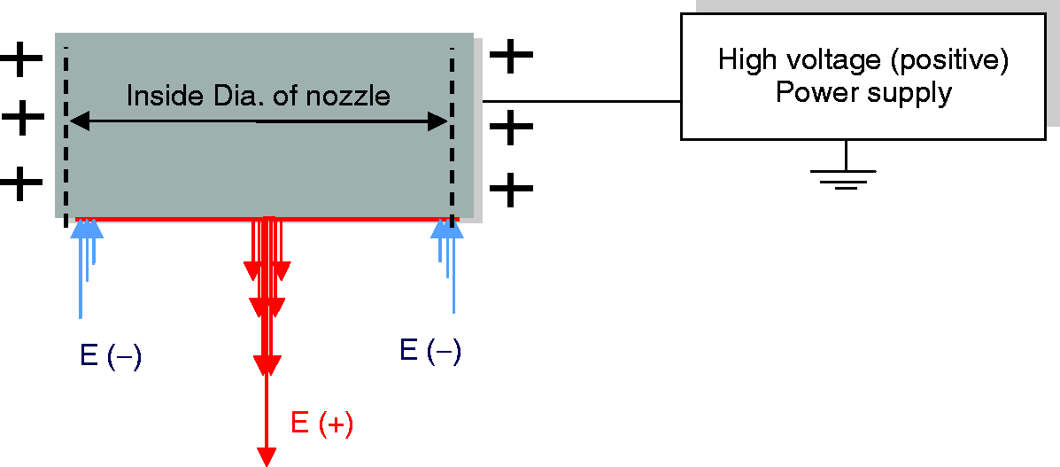

Stage 5: Interaction of the electric field vector distribution between the charged solution and the negative electrode (collector) with respect to side view B-B

The combined electric field vectors and the distribution of positive and negative ions as well as the neutral species before and after applying positive external electric field within the solution is illustrated in Figure 9. At this stage, once the positive external high voltage is applied, the effect of the negatively charged collector on the solution emerging from the end of the nozzle is considered. Here again, based on Coulomb's force of attraction, the net positive charge accumulated at the tip of the nozzle has a strong attraction towards the uniformly distributed negative charge of the collector.

Figure 9.

Schematic of collated ions at nozzle tip when subjected to external electric field.

However, at the same time, the negative charges accumulated around the walls of the nozzle end (Figure 9) are affected by the repulsive forces of the collector. Given that the negative charges on the inner wall of the nozzle end are uniformly distributed, the overall force of attraction between the positive ions focused in the centre of the nozzle and the collector are much stronger, thereby forcing the solution towards the collector. However, the resistance offered by the solution's surface tension causes the combined effect to form a cone-like profile known as the Tailor Cone. The concentration of the positive charges and their respective forces of attraction by the negatively charged collector increases when the amount of applied external voltage is between 5 and 6 kV [15]. Under these circumstances, the resistance due to surface tension holding the charged ions and the neutral species gradually diminishes due to the thinning of the surface tension layer, as highlighted by the thick and thin lines (shown in green, Figure 9). Eventually, the solution is allowed to escape from the apex of the cone where surface tension has become minimal. As the solution escapes, the overall surface tension at the tip of the cone is largely unaffected, i.e. the structure does not collapse.

The schematic shown in Figure 9 is an idealized example of the state of affairs; in reality, the polarized chains of neutral species maybe more intertwined (physically or chemically) and would form many sub-splays (see Figures 1 or 10(d)) after the formation of the initial splay.

Figure 10.

(a)–(c): Micrographs of electrospun poly(ethylene oxide) solution at different polymer concentrations.

Stage 6: Overall view of nanofibre formation between the positively charged nozzle and the negative electrode (collector)

Once released from the effects of surface tension, the aligned chains of polarized ions tend to repel one another due to repulsive forces that are greater in effect than the attractive forces of the collector, leading to an umbrella-like explosion (splay). As the fibres travel towards the collector, the electrostatic forces between the splayed fibres and the collector become increasingly dominant (see Figure 11). Once the splay is formed, the resultant Coulomb forces act on the extruded material differently, causing a violent whipping action as the fibres head towards the collector. This action contributes towards drawing of the fibres increasing their surface area, which also allows the solvent to evaporate. The net result is the formation of random deposition of the nanofibres on the collector surface.

Figure 11.

Step-by-step schematic of electrospinng process.

It is physically very difficult to photographically capture the instantaneous downward motion of the charged polymer droplet and its subsequent splay into individual segments heading towards the negatively charged target. The micrographs shown in Figure 10(a)–(c) are the closest one can get to these state of affairs. Figure 10(a) represents the spiral motion of a single nanofibre post splay formation when polymer concentration is relatively low. Figure 10(b) represents a more pronounced helical motion of a more concentrated polymer solution and Figure 10(c) shows multiple helixes due to even higher concentrations at higher applied voltage.

Stepwise progression of the solution from start to the point of dispersion into splay formation under the influence of critical voltage (i.e. >5 kV) is depicted in Figure 11 (A to H).

In the case of a stationary collector plate, the amount of fibres collected directly below the nozzle is greatest and reduces as the nanofibres settle away from this area, thereby affecting nanofibre deposition density.

Real images are extremely difficult to capture; however, what has been achieved provides the best factual evidence of the state of the affairs and hence complements the electrostatic model theory discussed in this article.

Conclusion

Electrospinning process is a complex phenomenon governed by the dielectric constant of the solvent, applied voltage, speed of production, delivery rate, solution concentration, feeding source, fibre diameter as well as distance between the charged feeding source and the target. However, under all circumstances, electrostatic forces play an independent and crucial role in forming the nanofibres and influencing their characteristic behavior. This article has attempted to demonstrate the role of electric field and electrostatic forces, from the first principles, in generating nanofibres from moment of inception to deposition on a stationary collector plate. The schematically traced evolution of the molecular motion of the charged species has elucidated the charge dispersion characteristics of the solution and its subsequent electrostatic behavior when subjected to high-voltage electric field. Under such circumstances, the concentration of net positive charges at the tip of the nozzle facing the uniformly distributed negative charge of the collector are very high, thus forcing the solution out of the nozzle. Tailor Cone formation is as a direct result of this force of attraction surrounded by the solution surface tension. Once the surface tension is pushed to its limit, the polymer escapes from the thinned out crust at the apex of the cone in the form of fine strands. The repulsive forces between the fine strands make them split into nanofibres showering down towards the negative target. The actual spinning process captured by the slow-motion camera has thus far provided some evidence in support of the explained theory but further research work is in progress to fully confirm the theory. These findings complement previously published [16–18] theories associated with electrospinning, which are essential in understanding the complex and the intricate balance of competing forces so that nanofibre formation and their manipulation could be better controlled and influenced. In our next article, the actual extrusion process with respect to the electrostatic theory described here will be used to generate predictive models covering the entire electrospinning process.