Swirling Flow Quantification in Helical Stents Using Ultrasound Velocimetry

Abstract

Objective:

Helical stents have been developed to treat peripheral arterial disease (PAD) in the superficial femoral artery (SFA), with the premise that their particular geometry could promote swirling flow in the blood. The aim of this work is to provide evidence on the existence of this swirling flow by quantifying its signatures.

Materials and Methods:

This study consists of in vitro and in vivo parts. For the in vitro part, 3 helical stent models of different helicity degrees and 1 straight model were fabricated, and the flow was assessed at the inlet and outlet of each model. For the in vivo part, only 1 patient, treated with the helical stent, was eligible to participate in the study. The stent implanted in the SFA of the patient was evaluated in 2 leg postures (straight and flexed), and flow was assessed in 12 locations along the SFA. The in vivo study was approved by an ethical board (NL80130.091.21) in the Netherlands. High-frame-rate ultrasound was used to acquire data from the regions of interest (ROIs), using microbubbles as contrast agents. After processing the data via a correlation-based algorithm (echo particle image velocimetry or echoPIV), the velocity vector field within each ROI was extracted and analyzed for parameters such as vector complexity and velocity profile skewedness.

Results:

The results show that in the outlet of the helical stents, when compared with the inlet, the flow vector field is more complex and the velocity profile is more skewed. For the in vivo case, the outcomes demonstrate more complexity and higher variability in the sign of skewedness inside the stent when compared with the flow in the proximal to the stent.

Conclusions:

Helical stents make the vector field of the flow more complex and the velocity profile more skewed, both of which are signatures of swirling flow. Further studies are needed to evaluate whether these features can benefit patients in terms of patency rates.

Clinical Impact

This study demonstrates that helical stent models alter the blood flow when compared with straight stent models. Particularly, the flow grows more complex and its velocity profile becomes more skewed, both of which hint at the existence of swirling flow inside the helical stent. These observations, alongside with population-based studies that are currently being carried out, may provide the evidence that helical stents have some advantages over straight stents for the patients.

Introduction

Peripheral arterial disease (PAD) is a subcategory of cardiovascular diseases (CVDs), with a worldwide prevalence of about 10% across demographic groups. ¹ CVDs are the leading cause of death globally, ² while significantly lowering quality of life for those affected. Research has shown that a fundamental change in lifestyle can not only prevent this disease ³ but also help reverse it, reviving normal arterial function. ⁴ According to the largest study of its kind, among the risk factors for CVD, diet and smoking top the list. ⁵ In the case of atherosclerosis, which accounts for 95% of all cases of PAD, plaques develop in the arteries that carry blood to the extremities. These plaques can cause progressive stenosis or occlusion in the arteries. As the disease progresses, symptoms vary from intermittent claudication to chronic limb ischemia that may consist of rest pain and/or necrosis, which in turn may lead to major limb amputation.

In addition to lifestyle modifications, ⁶ treatment options vary from pharmacological to endovascular and surgical interventions. To manage the symptoms, walking exercises and medication are often prescribed ⁷ ; however, if the disease progresses into more advanced stages, endovascular or surgical interventions are considered. In most severe cases, where, e.g., multiple stenoses or occlusions occur, open surgery is recommended, whereas in other cases endovascular approaches are preferred. ⁸ Percutaneous transluminal angioplasty (PTA) or plain balloon angioplasty (PBA) is a common endovascular option, often accompanied by nitinol stent placement. ⁸ The performance of nitinol stents decreases with the length and complexity of the lesion and therefore alternative strategies have been developed, including balloon-expanding stents, self-expanding stents, and drug-eluting stents, which are coated with slow-release medication to delay the formation of in-stent clots. ⁹

Besides their coating, the geometry of nitinol stents may have an important role in their efficacy, as the shape of the stent could affect flow parameters both inside the stent ¹⁰ and at its outlet. Most stents currently used are simple flexible cylinders, but recently, helical stents have been developed for the superficial femoral artery (SFA). These stents are designed based on the hypothesis that a helical shape could retrieve part of the swirling flow that exists in native vessels, which typically possess curves and twists^11,12 unlike vessels treated with straight stents. The promotion of swirling flow could also increase wall shear stress (WSS), which could be beneficial in delaying restenosis. ¹³ In the first MIMICs trial in 2018 with a population of 76 people, comparing patients who received a helical stent with those who received a straight one, the 2-year primary patency was shown to be higher in the helical group (72%) vs the straight-stent group (55%). Larger studies including more patients are currently being carried out. ¹⁴

Apart from patency outcome studies, empirical investigations into blood hemodynamics within helical stents are valuable in that they can show how effectively these stents can induce swirling flow. Recently, ultrasound (echo) particle image velocimetry (echoPIV) has been used to study blood flow both in vitro ¹⁵ and in vivo. ¹⁶ In the work at hand, echoPIV is used for the first time to detect and analyze signatures of swirling flow across the lumen of stented tubes and arteries. In a preliminary study of Dean flow in curved tubes, it was shown that echoPIV can capture a skewedness in the velocity profile across the diameter of semicircle tubes. ¹⁷ This skewedness is caused by the inertial forces due to the semicircle turn in the tube, and similar dynamics are expected to occur in helical stents due to their spiral shape. Another potential signature is the strength of the secondary flow in the lateral direction (with respect to the centerline of the tube). Vector complexity, which is a cumulative measure of the deviation and diversity of the vector angles from the centerline of the tube, ¹⁸ is used for this purpose.

This article focuses on measuring these 2 key signatures, i.e., skewedness and vector complexity, to quantify swirling flow in 3 helical stent models with 3 degrees of helicity and compare the results to those of a straight model. Various degrees of helicity, as provided by the manufacturer, represent values expected in the SFA in a flexed and straight leg as well as a posture in between.^11,12 The 3 hypotheses of this investigation are: (1) echoPIV is able to capture and quantify the differences in skewedness and vector complexity across models, (2) swirling flow causes the flow vector field to become more complex in the outlet of the helical models compared with that in their inlet as well as in the helical models vs the straight model, and (3) swirling flow causes the velocity profile to skew across the diameter of the helical models. These hypotheses were tested by measuring the flow at the inlet and outlet of all the stent models. In addition to this in vitro investigation, the aforementioned metrics are used to analyze the flow in vivo, in the inlet and inside of a stent implanted in the SFA of a patient.

Methods

The In Vitro Flow Setup

The flow setup (Figure 1A) consisted of a programmable piston pump (Super Pump, Vivitro, Victoria, Canada), to create pulsating flow; ultrasonic flow sensors (SonoFlow, Sonotec, Halle, Germany) in the up-stream and down-stream of the stent model; an in-house electronic valve; an in-house compliance, to mimic distal vascular compliance; and a reservoir containing blood-mimicking fluid (BMF) mixed with contrast bubbles, also produced in house. ¹⁹

Figure 1.

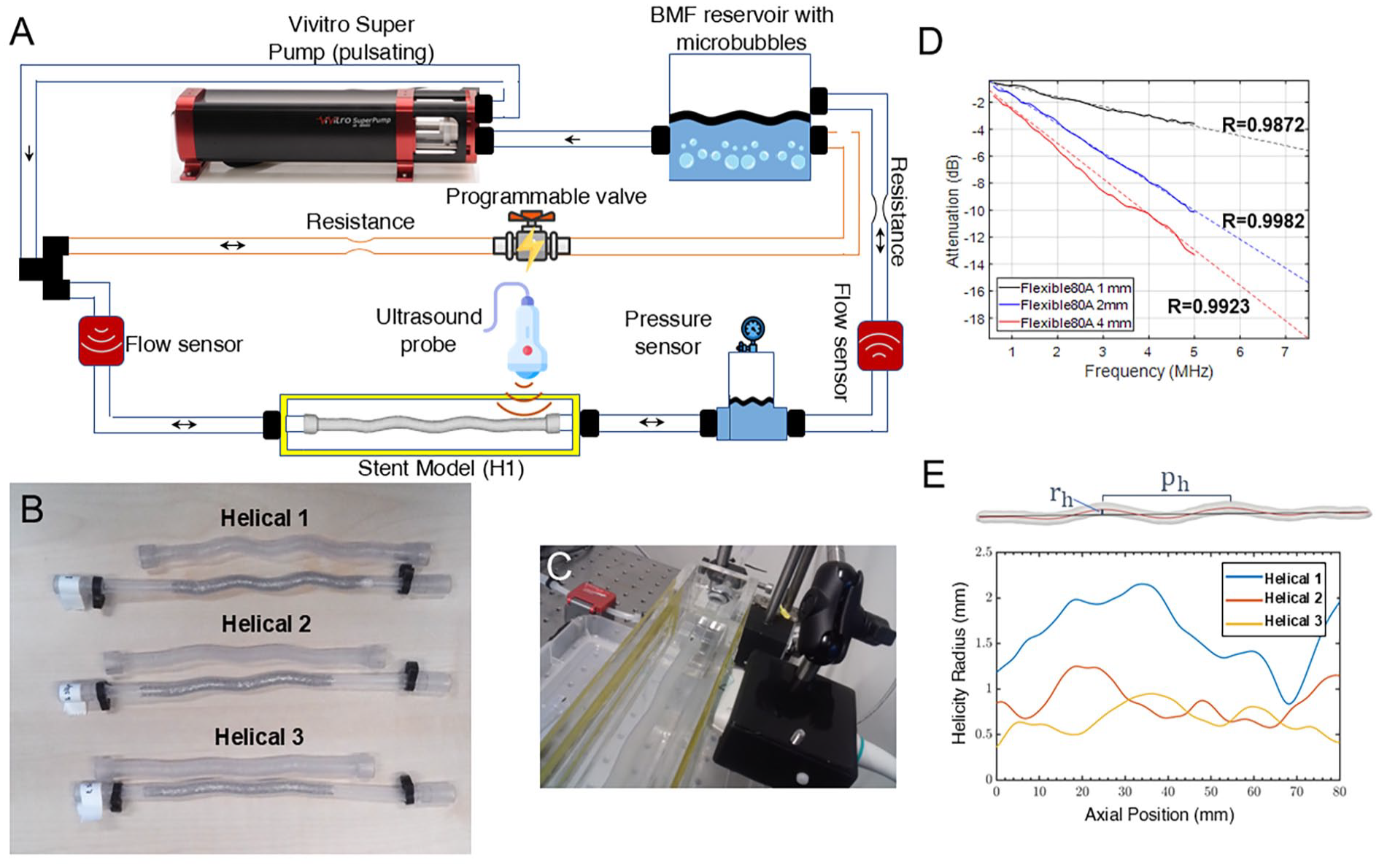
(A) A schematic of the entire experimental setup. (B) The 3D-printed stent models (Helical 1 to 3) and their corresponding stented thin-walled tubes. The added sleeves on the 3D-printed models allow for an easy connection to the flow setup and to have a straight section for a methodic measurement of the flow across various cases. (C) Ultrasound data acquisition via a window on the side of the small tank containing the stent model. (D) Attenuation plots of thin slabs of Flexible-80A measured at 0.5 to 5 MHz and interpolated with a power law to 7.5 MHz. (E) Helicity radius results alongside with a segmented geometry of a helical stent, its centerline (red), and the reference, rotation axis (black). The helicity radius is indicated by r_h and the helical pitch by p_h. [The diagram in (A) has been designed using images from Flaticon.com].

Four 3-dimensional (3D)-printed stent models (Figure 1B) were installed one by one in a water tank. Next, ultrasound images were collected both at the inlet and the outlet of the models (8 data sets in total—6 for the stent models and 2 for the straight one). A rigid acrylic tube was placed behind the inlet of the stent model to cover the length needed for fully developed flow. The tank had acoustically transparent windows made of thin plastic foils. The width of the tank was designed to be short to enable imaging the models from the side and within ±10 mm of the elevation focus of the ultrasound probe (Figure 1C).

Before imaging each model, 2 mL solution of in-house lipid-coated contrast bubbles, which were between 6 and 8 microns in diameter, was injected into the reservoir. The BMF recipe was adopted from the literature, ²⁰ with a water-glycerol volume ratio of 62/38, leaving out the urea. Here, urea was not used, because based on the literature, the assumption was that its main function is to modify the refractive index of BMF for laser PIV. Yet, it became clear to us later that urea also acts as an anti-fungal agent and it is thus recommended to be used. The 62/38 ratio leads to a density of about 1100 kg/m³ and a viscosity of about 4 mPa s for the BMF. To acquire and record the data, a fully programmable ultrasound system (Vantage-256, Verasonics, Kirkland, Washington) and an L12-3v ultrasound probe (Verasonics) were used. The frequency of the probe (number of elements: 192, sensitivity: −58.4 dB, elevation focus: 20 mm) was set at the center value, f_c=7.5 MHz, with a maximum voltage of V=5 V. To realize high-frame-rate (HFR) acquisition at 2000 fps, the Verasonics system was configured to perform plane wave imaging for a duration of 4 seconds, in order to cover at least 3 full cardiac cycles. A probe holder was designed and 3D-printed to stably position the ultrasound probe and align it with the central plane of the lumen of the helical and straight models, Figure 1C.

Flow rate and profile

The mean flow rate in the SFA has been reported to be near 150 mL/min (2.5 mL/s);^21,22 therefore, the pump’s output stroke power was adjusted accordingly, monitored by the sensor at the inlet of the models. The pump was programmed to generate a flow profile as typically observed in the SFA. ²² As the pump could only create flow in 1 direction, the electronic valve was synced with the pump to create backflow. It was noted that even without the electronic valve running, simply because of having a second path in the flow, adequate backflow was generated, which was enough to mimic the cardiac cycle in the SFA. Moreover, 2 additional resistances (surgical clamps) were used to tune the flow profile to match that found in the literature. ²²

Stent models

Three helical stents (BioMimics 3D Vascular Stent System, Veryan, Horsham, UK) were deployed in thin-walled elastic tubes in different configurations so that each has a different degree of helicity, corresponding to various human postures. ¹¹ The stents were 15 cm in length and 7 mm in diameter. The effect of torsion and twist, which has been documented in native vessels, ¹² was not considered in this study. As the thin-walled tubes were inflatable and could not withstand the pressure values in the flow setup, the geometries of the stented tubes were recreated in a 3-step process. First, the stented tubes were scanned with computed tomography (CT) (Artis Pheno, Siemens AG, Berlin, Germany, spatial resolution 0.47 mm), and their geometry was captured in 3D. Second, the stented tube geometries were reconstructed in a mesh (STL) format, followed by a threshold-based segmentation. Third, the models were 3D-printed with a flexible resin (Flexible-80A, Formlabs, Somerville, Massachusetts), after tubulation at a thickness of 1 mm and adding a straight length of 20 mm on the both sides. Figure 1B shows an image of each 3D-printed stent model alongside its original stented tube. The extra 20 mm length on both ends of each tube was added to enable planar ultrasound imaging and the inlet-outlet comparison. This was done because the helical part of the models could not be imaged within a single plane in all the cases, due to the out-of-plane parts of the geometry.

In addition to providing flexibility, Flexible-80A at a thickness of 1 mm provides a low enough attenuation to pass the ultrasound signal from the contrast bubbles through. To keep this level of flexibility and low attenuation, the printed models were cured in the ultraviolet (UV) oven for only 5 minutes. The attenuation of ultrasound waves (0.5-5 MHz) through thin and uniform slabs of Flexible-80A was also measured in a separate acoustic characterization setup, using room-temperature water as the reference. The attenuation ratio was interpolated assuming a power-law trend, as shown in Figure 1D. The interpolated attenuation was −5.6 dB at 7.5 MHz for a slab of 1 mm.

Helicity quantification

To rank the stents based on their helicity levels, a method was devised to quantify helicity. For this purpose, the geometry of the stent models was acquired by a CT scan, while they were installed in the container so that their shape was preserved as it was during the experiments. Using 3D-slicer (Slicer.org Version 5.2.2), ²³ the lumen of each model was segmented from the scans using a Fast-Marching algorithm. Subsequently, the lumen was smoothed and its centerline was computed by the VMTK toolbox in 3D-slicer. The helix radius of the centerline of each model was evaluated as a measure of helicity. A line representing the rotation axis of the helix was constructed by fitting a straight line through the helical trajectory using a least-squares approach. For every point on the centerline, the helicity radius r_h was defined as the length of the line segment that connected the centerline point with the helical axial axis and was orthogonal to the reference (rotation) axis (Figure 1E). In addition, the helical pitch was measured as the distance between 2 peaks.

The helicity radius for the 3 stented models is plotted in Figure 1E, ranking the models from the most to the least helical. Helical 1 shows the largest helical radius (average 1.61 mm), with a declining radius for Helical 2 (average 0.83 mm) and Helical 3 (average 0.66 mm). The measured helical pitch for Helical 1, 2 and 3 was 47.4, 48.5, and 56.3 mm, respectively.

Patient Study

The in vivo study (prospective) was approved by a certified ethical committee (NL80130.091.21) and the institutional review board. One patient (57 years old, male), who had received the BioMimics 3D helical stent, was enrolled after signed, informed consent. The HFR ultrasound data (2000 fps, 3 angles) was collected in the middle, and at the inlet and outlet of the stent in vivo in 2 different leg postures: straight and flexed. The stent was placed in January 2019, and the data was collected in March 2023. The patient received a 0.75 mL intravenous bolus injection of SonoVue microbubbles (Bracco, Milan, Italy) prior to the HFR acquisitions, as contrast agents. To allow for deeper imaging within the tissue, a frequency of 4 MHz was used, with the L11-4v probe (Verasonics), in contrast to the 7.5 MHz used during the lab experiments. Furthermore, a computed tomography angiography (CTA) scan was obtained to assess the SFA and stent geometry.

Analysis Technique

Echo particle image velocimetry

In echoPIV, the movement of contrast microbubbles—which appear as submillimeter speckles in an ultrasound image—is recorded using HFR ultrasound. Then, the acquired images are processed using a correlation-based algorithm, ²⁴ which results in a velocity vector field in the region of interest (ROI).

In the in vitro study, on the average ultrasound image for all the frames, a mask of 6 mm× 10 mm (spanning the entire diameter of the printed models and extending 10 mm along their axis) was selected as an ROI for echoPIV. This ROI was defined closest to the sleeve of the printed models in the inlet and closest to the helical section in the outlet. Next, the acquired image data was processed with the echoPIV algorithm to compute the 2D velocity vector fields. In calculating the correlation values, 4 passes were used and the kernel sizes in each pass were, respectively, 64×64, 32×32, 16×16, and 16×16, defined in pixels. In the output, each vector field (ROI) had 26 and 38 vectors in the lateral and longitudinal directions. Having this fixed ROI size allowed for a better comparison of the mean metrics across cases.

In the in vivo study, due to the complex geometry of the SFA and the varying quality of data in different locations of the image, choosing an ROI with a fixed number of pixels was not feasible. Furthermore, after image reconstruction and singular-value-decomposition (SVD) filtering, ²⁵ it became apparent that the data at the outlet of the stent could not be analyzed due to low signal-to-noise ratio (SNR) in that region. The same held for the image set from the flexed leg position, around the inlet of the stent. Therefore, for the patient data, 12 ROIs with sufficient SNR were selected and analyzed: 4 ROIs in the stent-inlet image set, straight leg position; 4 ROIs in the mid-stent image set, flexed leg position; and finally, 4 ROIs in the stent-outlet image set, flexed leg position.

Skewedness and vector complexity

The methodological details of the 2 quantitative parameters, i.e., skewedness (S) ¹⁷ in the velocity profile and modified vector complexity (MVC) in the vector field ¹⁸ —measured and analyzed in both the stent models and the implanted stent in the patient’s leg—are given in Supplementary Materials B. A 2-tailed t-test was used to assess the significance of the difference for each quantitative parameter between 2 data sets (e.g., inlet and outlet of a stent).

Numerical Study

In 2-dimenisonal (2D) ultrasound imaging, data are acquired from only a particular plane passing through the ROI. As swirling flow is a 3D phenomenon, the values of MVC or S depend on the selected imaging plane. This dependency could affect the comparison made between the values of these parameters at the inlet and outlet of a stent model. Similarly, the plane angle can also affect the comparison across stents. Studying different imaging angles was not feasible in the experimental setup. Hence, to study the mentioned dependency, a numerical simulation was carried out in COMSOL Multiphysics on a helical geometry, reconstructed from the most helical case (unrestrained at the ends), with a helix radius of a=18 mm and a pitch of p=46 mm. Similar to the in vitro study, a typical flow profile of the SFA ²² was used as an input for the flow simulations. Vector fields were extracted at the inlet and the outlet for various plane angles from θ=0 to θ=170° at intervals of ∆θ=10°, relative to a reference plane passing through the axis of the helix.

To compare the results of the in vitro study with the numerical results, the helical stent models (Helical 1 to 3) were CT-scanned while installed in the flow setup and their geometries were recreated as an input to COMSOL Multiphysics for a time-dependent study. Numerical studies of swirling flow have been previously reported for helical stents, ²⁶ stent grafts,^27,28 and native vasculature ²⁹ in the body. For the aforementioned comparison, similar to the in vitro study, both S and MVC were measured at the inlet and outlet of each stent model. Furthermore, flow helicity ²⁷ (different from geometrical helicity in Figure 1E) was calculated for all the helical stents. The details of this study and its results are presented in Supplementary Materials C.

Results

In Vitro Analysis

The vector field outputs of the echoPIV algorithm for the most helical stent (H1) model are shown in Figure 2A and B as 2 time-averaged vector fields. The vector fields as a function of time can be viewed as a video in the Supplementary Materials D for the outlet of H1, as an example. Figure 2C and D depict skewedness in the velocity profiles, across the diameter of the tube, where the shaded area is bounded by the maximum and minimum profiles (in time and along the tube) in light red. The solid line within the shaded area represents the spatiotemporal mean velocity profile, averaged over time and along the axis of the stent model. Figure 2E shows a comparison among different methods obtaining the flow rate at the inlet of the most helical model (Helical 1) as an example. As shown, the flow rate value, as recorded by the sensor Q_sensor, was 3.052±0.03 mL/s, averaged over 1 full cycle with the standard deviation reported for 3 cycles. This matched well with the maximum flow rate (the center of the ROI), as computed by echoPIV (Q_echoPIV,mp=3.310±0.04 mL/s, 8% difference), but had a larger difference with the echoPIV flow rate averaged over the diameter of the stent model (Q_echoPIV,m=2.287±0.04 mL/s, 25% difference).

Figure 2.

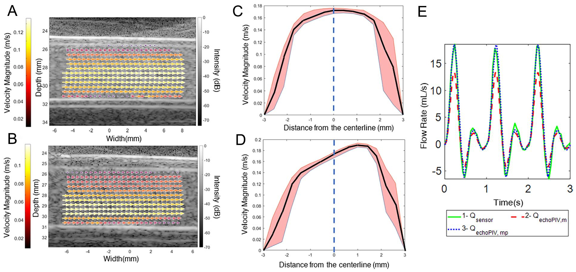
Flow output, vector fields, and skewedness. (A) and (B): An example of a vector field, averaged over time and color-coded, in the (A) inlet and (B) outlet of Helical 1. (C) and (D): An example of a velocity profile in the (C) inlet and (D) outlet of Helical 1, averaged over time, and later averaged along the length of the ROI (solid line). The shade depicts the bounds of the minimum and maximum profiles, and the solid line shows the mean velocity profile, over the ROI length and time. (E) A comparison between the flow sensor data (Q_sensor) and echoPIV data (Q_echoPIV,mp, at the central point of the ROI, and Q_echoPIV,m, averaged over the diameter of the tube) (see Supplementary Materials D for a video of the vector fields as a function of time).

Figure 3 shows the results of the analysis on MVC and S for all the inlets and outlets of the stent models. Several observations can be made considering Figure 3A: (1) MVC is higher in all helical models than in the straight model, both in the inlet and the outlet; (2) MVC is significantly higher in the outlet of the helical models when compared with their inlets (72.4%, 20.8%, and 15.72% for H1, H2, and H3, respectively), whereas this difference is negligible in the straight model (4.72%); and (3) MVC is the highest in the most helical model (H1). When helicity decreases (to H2 and then H3), MVC does not necessarily decrease (see section “Discussion”), but the difference in MVC between the inlet and the outlet is the highest in H1 and the lowest in H3. Figure 3B shows that the ratio between the MVC in the outlet and inlet is the highest in H1 and the lowest in the straight model.

Figure 3.

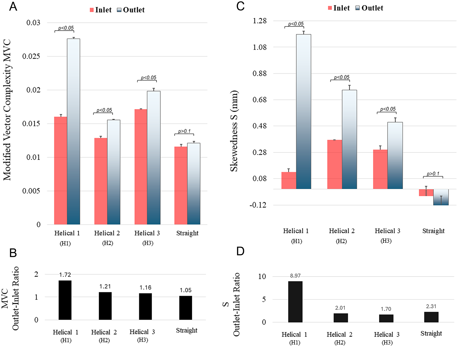
Comparison between the inflow and outflow of 3 helical stent models and 1 straight stent model: (A) modified vector complexity (MVC, unitless), (B) the ratio of MVC at the outlet to the inlet, (C) skewedness (S, mm), and (D) the ratio of S at the outlet to the inlet. The error bars in (A) and (C) represent the standard error, and the p-values show a significant difference between inlets and outlets of all models, except the straight one.

Similar trends can be observed in Figure 3C: (1) S is the highest in the outlet of the most helical model (H1) and S is higher in all the helical models when compared with the straight model, both in the inlet and the outlet; (2) the absolute difference in S between the inlet and outlet of helical models is 1.04, 0.377, and 0.21 mm, from H1 to H3, respectively, compared with 0.053 mm in the straight model; (3) S in the outlet decreases as the helicity decreases from H1 to H3, as opposed to S in the inlets of H1 to H3, which does not exhibit the same trend. It is noticeable that S is negative in the straight model, which means that the velocity profile is slightly skewed in the opposite direction of other models. Figure 3D depicts the ratio between S in the outlet and inlet. This ratio is the highest in H1.

In Vivo Analysis

Figure 4 shows the results of the patient data analysis, alongside with the average ultrasound images and the 12 selected ROIs on the left (Figure 4A–C). Each ROI is labeled with a number from 1 to 12, and the corresponding MVC and S values are shown in Figure 4D and E. As mentioned before, ROIs 1 to 3 are chosen as far as possible from the inlet of the stent (yellow arrow). ROI 4 is situated right after the inlet of the stent, with the effect of having a very high MVC and a very low S, compared with ROIs 1 to 3. As Figure 4E illustrates, S does not necessarily increase while passing through the stent alongside the flow, but its sign can change from one ROI to the other. This is not the case outside the stent and away from its inlet. Figure 4F shows the mean MVC for 3 different cases: (1) stent inlet, straight leg position; (2) inside the stent, straight leg position; and (3) stent inlet, flexed leg position.

Figure 4.

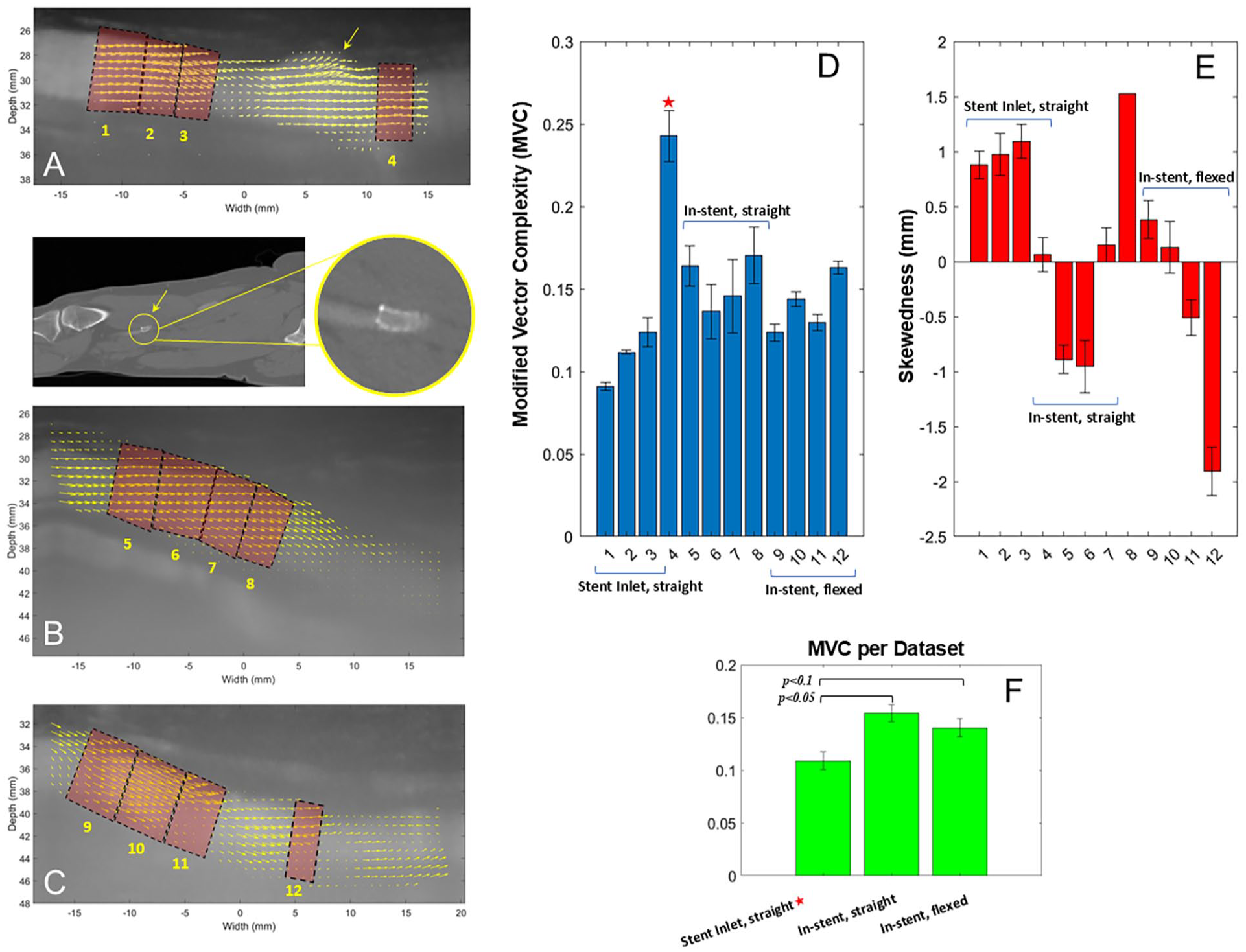
Flow characterization in a helical stent inside the superficial femoral artery of a patient. Twelve regions are defined: (A) 4 in straight leg position, proximal to the stent and at the inlet of the stent, (B) 4 inside the stent, in straight leg position, and (C) 4 inside the stent, in flexed leg position. (D) Modified vector complexity (MVC) and (E) skewedness (mm) for all the 12 regions. (F) Mean values of MVC for each data set, pertaining to (A), (B), and (C).

Numerical Analysis

Figure 5 shows the layout and results of the numerical study on an exemplary helical model. As shown in Figure 5A, the angle (θ) of the plane passing through the centerline of the inlet incrementally changes with respect to the z-axis (Figure 5A inset). Figure 5B and C show the extracted vector fields at the outlet and the inlet of the model for when θ=150°, spanning an area of 10 mm by 6 mm, similar to the in vitro settings. The calculated MVC and S for each plane angle are shown in Figure 5D and E. The ratio of MVC and S in the outlet to the inlet is also plotted, showing high variability across the planes.

Figure 5.

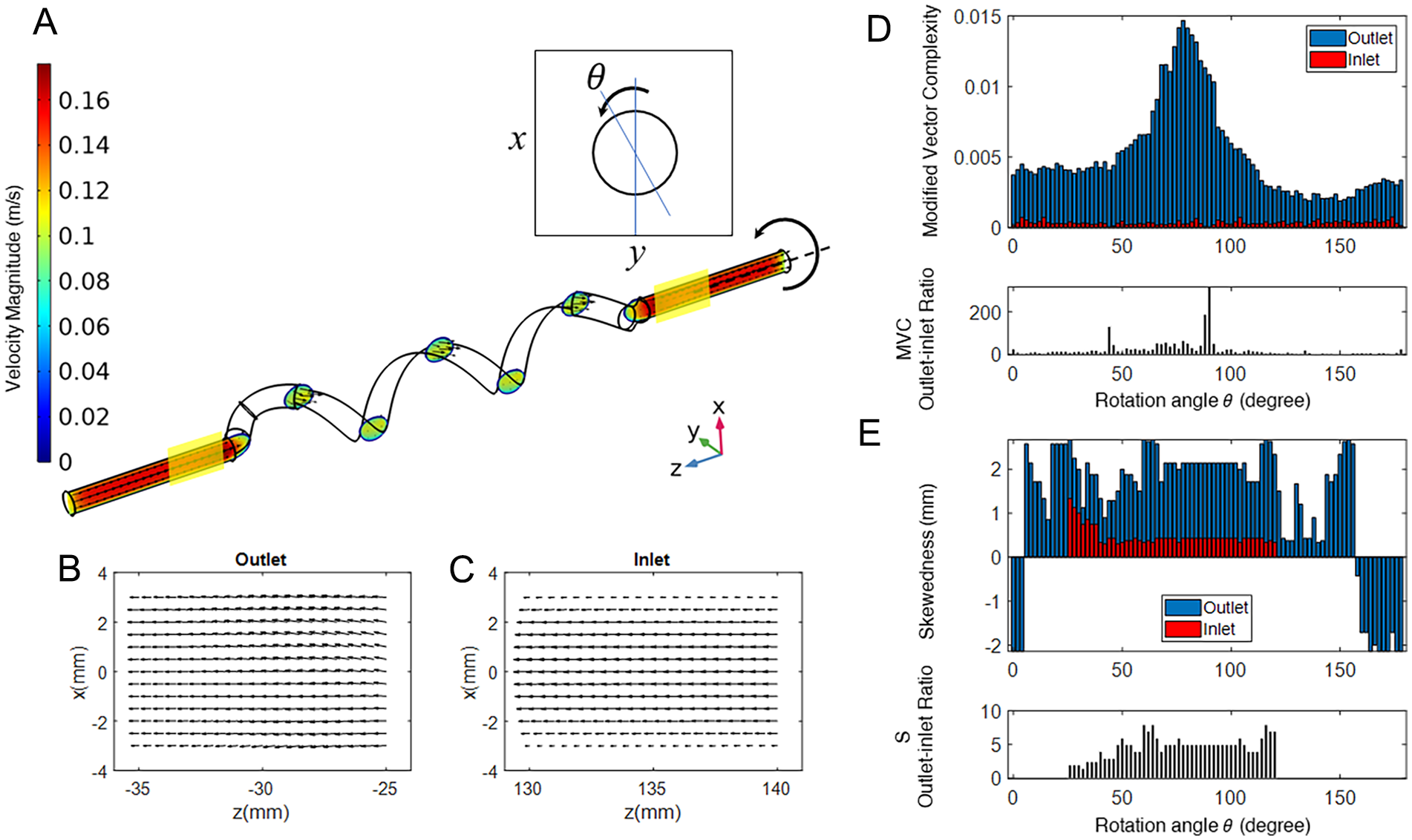
Effect of the angle of the plane around the axis of the stent on modified vector complexity (MVC) and skewedness (S): (A) An exemplary helical model simulated in COMSOL Multiphysics with a cardiac cycle, obtained from the superficial femoral artery, as input. The model is incrementally rotated around the z-axis, whereas MVC and S are measured in the 2 vertical planes (shown in transparent yellow); the vector field in the (B) outlet and (C) inlet planes for θ=150°, as examples; (D) MVC and its outlet-inlet ratio and (E) S and its outlet-inlet ratio as functions of the planar rotation angle (θ).

Discussion

The results show that, in general, vector complexity increases inside or at the outlet of the helical stents, when compared with the vector field at their inlet. The in vitro results show that skewedness is also increased due to the helical geometry of the stents. Within the stent, as the in vivo results reveal, the sign of skewedness changes alongside the stent in the helical section. The outcomes further demonstrate that echoPIV is a proper tool to detect relatively small differences in vector complexity and skewedness between helical and straight-stent models.

In Vitro and Numerical Results

Based on the results in Figure 3, one can conclude that the 3 main hypotheses are confirmed: (1) echoPIV can capture the differences in vector complexity (MVC) and skewedness (S) between the inlet and outlet of the helical stent models and in comparison to the straight-stent model; (2) and (3) the helical shape increases MVC and S in the outlet of the helical stent models. The MVC and S are also higher at the inlet of the most helical case (H1) when compared with that in the straight model, which could be an indication of backflow, likely caused by the helical shape. The backflow relates to the concept of hydraulic resistance and energy dissipation, which is reported to be higher in helical vessels.^29,30 This may also implicate that there is an optimal rotation at the entrance of a helical stent to minimize energetic losses while the blood transitions from the native vessel into the stent. ³⁰ In large arteries, energy dissipation within a helical flow has been reported to reduce the risk of stent-graph migration. ²⁹

In Figure 3, it is noticeable that MVC and S do not necessarily increase when helicity goes up (notice MVC in the outlet when going from H2 to H4, and S in the inlet when going from H1 to H2). This is most likely because of the dependency of MVC and S values on the angle of the imaging plane, as mentioned in the numerical study.

The results of the numerical study in Figure 5D and E verify that in a helical model, MVC is always higher in the outlet than in the inlet in the same plane and across rotated planes. This is consistent with previous studies where regions with high circulatory flow (e.g., around stenoses) exhibit higher vector complexity values. ³¹ In a way, swirling flow is a secondary circulation (cross-sectional) moving along the primary flow (longitudinal), whose effect can be seen in the MVC in the outflow, where part of the swirling flow still exists. For the same plane (at a constant θ), S is also always higher in the outlet than in the inlet. Nonetheless, there are a few cases where S in the inlet of a certain plane goes beyond that in the outlet of another plane. Based on these, as long as a similar plane is selected in the inlet and outlet, experimental observations should have the same trend. This is also true when comparing a helical model with a straight one. It can be seen that in the numerical results (Figure 5), the ratio of MVC or S in the outlet to the inlet is variable across plane angles. Therefore, taking the ratio is still susceptible to the choice of the plane, as briefly discussed in the in vitro results (Figure 3).

Higher skewedness in the velocity profile of the outflow is consistent with studies of flow in curved geometries. ³² Also, skewed velocity profile has been studied in the common carotid artery (CCA), showing that even small curvatures in the CCA can cause measurable secondary flows and skewedness in the velocity profile. ³³ Velocity profile skewing has been reported to cause meaningful errors in the estimation of maximum velocity in the blood flow using Doppler imaging. This is due to the assumed link between flow rate and maximum velocity, which is invalidated in the case of a skewed velocity profile. ³⁴ In echoPIV or vector flow imaging, this problem is minimized as the velocity profile can be extracted from the resulting vector field.

Returning to Figure 3, it is clear that, as the numerical results predict, MVC and S are always higher in the outlet than in the inlet. But across stents, which have been imaged at arbitrary planes, this does not hold true. For example, S in the imaged plane at the inlet of H1 is lower than S in the imaged plane at the inlet of both H2 and H3. Thereby, it can be concluded that the 2D method devised in this study is only suitable for comparisons made within the same plane and cannot be used for comparison across different helicity levels unless multiple planes at different angles are imaged and processed.

Regarding the ratio of S and MVC in the inlet and the outlet, Figure 4B shows that the MVC outlet-inlet ratio decreases as helicity decreases. It can also be observed in Figure 4D that the ratio of S in the outlet to the inlet is the highest in H1 and the lowest in H3. However, despite the small values of S in the straight case (outlet: −0.12, inlet: −0.053), the ratio is higher than that in H2 and H3, meaning that taking the ratio is not a good representative of the level of velocity profile skewedness in these models. This is again due to the planar dependency of these values.

In Vivo Results

The interpretations of the in vivo results in Figure 4 are not as straightforward as the in vitro ones. It is important to note that when considering the helical part of the stent in the middle, the vessel centerline goes in and out of the plane, as do the velocity vectors within the field. Thus, the vector field within the stent—in that particular imaging plane—may exclude many of the vectors that point towards out of the plane, and this could affect the values of MVC and S. This was the reason that in the in vitro study, the helical part was not investigated.

However, the higher values of MVC observed inside the stent stand to reason as the helical shape of the stent should increase the variety in the angle of the vectors with respect to the centerline of the stent. One may expect MVC to be even higher than their current values, if the out-of-plane vectors could be included in the analysis.

In Figure 4E, the comparatively low value of S in ROI 4 requires more scrutiny. At this location, the skewedness may have decreased due to the straight section at the inlet of the stent, which may have organized the vectors in the field. However, the extremely high amount of MVC is most probably due to the misalignment between the stent axis and the SFA axis, in the inlet, as shown in the CT image under Figure 4A. This misalignment has caused some circulations (the yellow arrow) whose effect has lasted inside and at the inlet of the stent, thus increasing the MVC. Treating ROI 4 as an outlier (marked with an asterisk), and grouping the ROIs of each data set, one can compare average MVC across locations in Figure 4F. It can be seen that within the stent, MVC is higher than the values obtained from outside and proximal to the stent, in both the straight and flexed leg postures (p<0.1, p<0.05, respectively). Another observation is that in the in vivo results, the values of S are already relatively high (S>1 mm) outside the stent, which may be due to the native helicity of the SFA itself and other geometrical effects. The drastic change in the value of S within the stent due to the sign change is also consistent with one’s expectation about a swirling flow. As a flow swirls alongside a helix, the maximum velocity should shift from near one wall to the other, which can be the interpretation of what is observed in Figure 4E. This, however, was not observed in the results of the in vitro study, which were only assessed at the inlet and outlet of the stent models. One reason maybe that the sign-changing effect of the swirling flow inside the stent was not strong enough to last in the stent outlet.

The in vivo results confirm the fact that the helical geometry of a stent makes the flow inside it more complex and cause the velocity profile to have highly varying skewedness alongside the flow, both of which could be signatures of swirling flow within the stent. It should be noted that these effects last long enough to be captured at in the outlet of the stent, as observed in the in vitro results. Spatial variations of the velocity field within the stent could also mean higher WSS. Owing to the existing noise in the lateral velocity and its influence on the accuracy of the derivative of velocity with respect to space, WSS was not evaluated in this study, but it should be considered as a subject for future research. The in vivo results, despite having available data from only 1 patient and more variety due to intricate geometry inside the body, demonstrate that the sign of S alters alongside the stent, which could indicate that the flow swirls as it progresses along the stent. Whether these effects are strong enough to make a difference in the primary patency of the stents and be beneficial for patients need to be confirmed by larger population studies.

As observed, the 2D ultrasound method devised in the in vitro study was also usable in an in vivo setting. However, the inlet and outlet of the stent models were well controlled to be straight in the in vitro investigation. This was not the case in the patient study, where the flow in the inlet and middle of the stent was also a function of the complex geometry of the SFA itself (curves, existence of mild plaques, etc). Regardless, valuable observations were also made from the outcome of the in vivo study, including the difference in the pattern in MVC and S, when comparing the flow at the inlet and in middle of the stent.

Echo Particle Image Velocimetry for Flow Visualization

It should be noted that echoPIV has several advantages when compared with other experimental fluid dynamic techniques. For example, unlike optical PIV, which requires transparent media, echoPIV can be used in patients. Also, in contrast to 4-dimensional (4D) flow magnetic resonance imaging (MRI), ³⁵ which generates average flow vector fields over 1 cardiac cycle—possibly averaging out some flow phenomena, echoPIV can acquire and analyze multiple cardiac cycles, the number of which is only limited by the amount of data that can be stored on the acquisition system. The 4D flow MRI is also susceptible to artifacts induced by metallic stents. ³⁶ What is more, ultrasound is cost-effective and more accessible than MRI, making echoPIV more appealing for blood flow studies, e.g., at bedside. Therefore, echoPIV is a suitable tool to study the flow generated by helical stents.

Of course, the would-be swirling flow inside helical stents is 3D by nature, and ideally echoPIV using 3D ultrasound ²⁴ can be used to quantify this 3D flow. However, acquiring and analyzing ultrasound data in 3D is both data-and time-intensive, and currently, the 3D acquisition apparatus is not as widely available as 2D ultrasound. Moreover, 3D echoPIV lacks the temporal resolution in terms of frame rate to fully resolve flow hemodynamics. Hence, in the study at hand, we focused on developing a methodology to quantify the 3D swirling flow using 2D ultrasound.

Conclusions

The results of our in vitro study on helical stents with 3 different levels of helicity showed that the helical shape increases vector complexity and skewedness, both signatures of swirling flow inside the stents. The in vitro outcomes were in agreement with the numerical results. Similar effects were observed in studying the blood flow in a helical stents inside a patient’s leg. Whether these observations would translate to better clinical outcomes in patients needs to be investigated in larger population studies, some of which are currently ongoing.

Supplemental Material

sj-docx-1-jet-10.1177_15266028241283326 – Supplemental material for Swirling Flow Quantification in Helical Stents Using Ultrasound Velocimetry

Supplemental material, sj-docx-1-jet-10.1177_15266028241283326 for Swirling Flow Quantification in Helical Stents Using Ultrasound Velocimetry by Ashkan Ghanbarzadeh-Dagheyan, Majorie van Helvert, Lennart van de Velde, Michel M.P.J. Reijnen, Michel Versluis and Erik Groot Jebbink in Journal of Endovascular Therapy