Sage Journals: Discover world-class research

Abstract

The free-list method has enjoyed a remarkably productive history, yet most free-list research is limited to informal comparisons that are heavily reliant on point estimates such as item or cultural salience. Here, we demonstrate a range of methods to incorporate uncertainty into such group-level estimates. This approach involves: (1) resampling individual-level data (via bootstrapping or Bayesian regression) to create a range of hypothetical alternative samples; (2) generating group-level estimates (e.g., Smith’s S) in each sample; and (3) using the variation in these estimates as uncertainty intervals. While we focus predominantly on cultural salience, this approach can be applied to other free-list metrics. We also present some extensions to this approach, such as comparing estimates between items and between groups. We provide open data and code to help readers gain familiarity with these methods. Ultimately, we encourage researchers using free-list data to move beyond simply reporting point estimates.

Introduction

As socially transmitted representational content stored in human minds (Boyd and Richerson 1988; D’Andrade 1981; Sperber 1996), culture and cultural data are central to the social sciences. Ethnographic free-listing is a common method for soliciting naturalistic, content-rich, ecologically valid cultural data about a target domain (Quinlan 2005). Many metrics exist that reveal and examine the important properties of culture that free-list data contain, but few applications incorporate uncertainty into their analyses (Purzycki 2025).

In a nutshell, free-listing entails that participants list things they associate with some topic (e.g., features of heavy metal music, ideal partner qualities, or all the teas they know; see Table 1). While the content and frequency of items tells us a lot about what people think, as the items individuals list are ordered, free-list data also contain important structural properties (i.e., how people think). As such, free-listing can bridge between qualitative and quantitative data and is uniquely catered to examine the content and structure of cultural models.

Table 1.

Example of free-list data with item salience, using “types of tea.” ‘ID’ is participant number, ‘order’ is order listed, ‘item’ is item listed, and ‘item.s’ is item salience.

ID	order	item	item.s
EX001	1	rooibos	1.00
EX001	2	green	0.67
EX001	3	Earl Grey	0.33
EX002	1	Earl Grey	1.00
EX002	2	green	0.75
EX002	3	Baker St.	0.50
EX002	4	mint	0.25
EX003	1	mint	1.00
EX003	2	green	0.83
EX003	3	camomile	0.67
EX003	4	Earl Grey	0.50
EX003	5	Cubbiwubbi	0.33
EX003	6	oolong	0.17
. . .	. . .	. . .	. . .
EX $x$	k	$i$	$s_{i}$

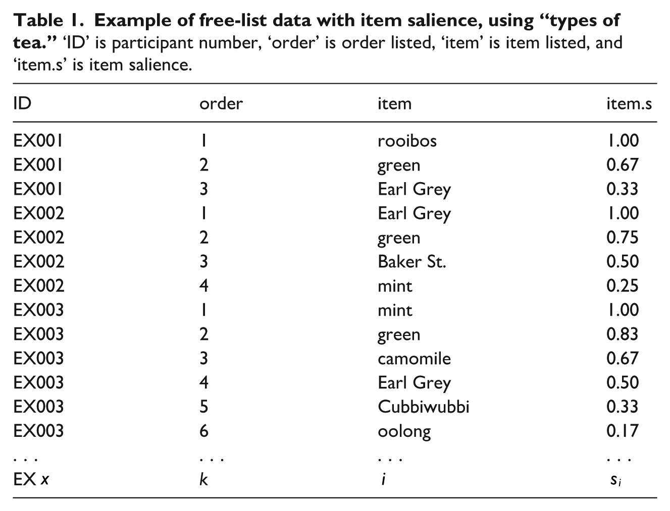
A key metric in free-list data is item salience, $s_{i}$ , which is a measure of an items’ accessibility or cognitive salience. One common way to calculate item salience, where $k_{i}$ is item order and $n$ is the number of items listed, is

s_{i} = \frac{n + 1 - k_{i}}{n}

Here, the first-listed items always have an $s_{i}$ score of 1, and each subsequent item salience is scaled based on how many items participants listed (e.g., 1, 0.67 and 0.33, if three items were listed). Depending on our goals, items not listed by participants might be given an $s_{i}$ value of 0.

These item saliences scores can then be used to examine cultural salience. Cultural salience (Smith and Borgatti 1997) bridges the gap between individual cognition and cultural distribution. A common way to calculate this is Smith’s S (see Sutrop 2001):

S = \frac{\sum s_{i}}{N}

where $N$ is the sample size so that whenever $s_{i} = 0$ , those individuals are included in its calculation. As such, Smith’s S is a scaled index of both accessibility and ubiquity. While other salience score calculations abound (e.g., Robbins et al. 2017; Sutrop 2001), Smith’s S is the most commonly used, has software already designed for its calculation, and—in our view and experience—remains the most intuitive and robust across conditions. We use it exclusively here, but the present discussion applies to all such metrics, including other measures of item salience (e.g., list frequency and list order; see Purzycki 2025), as well as those with similar properties (e.g., Jaccard’s similarity index or a cognitive sharing index like that in Robbins and Nolan 2019).

Researchers tend to report salience scores descriptively, and make informal comparisons with them (e.g., “This item is more salient than that one” or “Item X is more culturally salient for Group A than for Group B”). Yet analyses and interpretations that rely on point estimates can be unreliable and potentially misleading in a few key ways.

First, such analyses lack formality and rely on researcher intuitions and biases (however reasonable and correct they might be), rather than some principled and reproducible method. If an item, for example, had a salience score of 0.7 and another was 0.6, we must rely on our own hopes and interpretations to render a judgment about how different these items’ salience scores are.

Second, point estimates do not tell us how likely we are to get similar results if we repeated the study, providing a false sense of precision. A Smith’s S score of 0.30 from one sample could change to, say, 0.21, 0.17, 0.32, or 0.38 with other samples from the same population. Relatedly, point estimates do not provide any information regarding uncertainty; for instance, a Smith’s S of 0.5 in a large sample would be estimated with greater certainty than the same value in a smaller sample. Statistics like confidence or credibility intervals give us a better sense of how replicable and uncertain our point estimates are (Gelman and Greenland 2019).

Given these issues, making comparisons, contrasts, predictions, and causal estimates are severely hampered without embedding these salience scores into some principled approach that incorporates uncertainty into these estimates. Despite this, studies using free-list data frequently only report point estimates. Although recent case studies (Bendixen and Purzycki 2025; Purzycki et al. 2020) bring free-list data and their properties to bear in a probabilistic regression framework as outcome (i.e., dependent) variables, there remains a dearth of uncertainty estimates in purely descriptive and comparative studies. This article offers a few methods to address this lacuna.

Propagating Uncertainty

To make more principled descriptions and comparisons, then, we need uncertainty intervals (Gelman and Greenland 2019) around indices like Smith’s S. There are a few ways to do this.

One common way to generate uncertainty is to bootstrap (Efron and Tibshirani 1994). This involves randomly sampling a set number of observations with replacement from a sample (i.e., each observation is returned to the sample for potential resampling), then reporting the desired quantile values (e.g., 0.025 and 0.975 for the conventional 95% interval). This approach is simple and does not require declaring any particular distribution. Hence, it works regardless of the observed values. However, because it makes no distributional assumptions, the approach lacks any generativity that allows us to make inferences beyond our sample. In sum, while bootstrapping might be the simplest approach, it lacks principle and may be somewhat limited in use.

Another way is to calculate uncertainty intervals using a regression framework. Regression requires us to model the estimate using a particular distribution. While one could use either frequentist or Bayesian approaches, here we focus on Bayesian methods for three main reasons: (1) the interpretation of Bayesian credible intervals is more intuitive than frequentist confidence intervals; (2) many of the relevant distributions and situations we may wish to model are currently only available in a Bayesian framework (e.g., zero–one inflated Beta and ordered Beta models; discussed below); and (3) Bayesian models allow us to incorporate information regarding our knowledge and/or assumptions about the data (i.e., priors). For introductions to Bayesian regression, including best practice guidelines, exploring the assumptions of priors and convergence diagnostics, see Gelman et al. (2020) and McElreath (2020).

In the next section, we briefly introduce some options for propagating uncertainty around item and cultural salience scores. We then turn to an application and discussion with real data. To help readers replicate, understand and adapt these methods, full data and analysis code are available on our accompanying GitHub page (https://github.com/djsmith-90/FreeListUncertainty_CompanionCode; with additional technical details given in the longer preprint of this paper: Major-Smith and Purzycki 2025).

Methods

Because it has dedicated software for both processing free-list data and statistically modeling estimates like salience, the following analyses are conducted exclusively using R software (R Core Team 2023). To illustrate our steps and analyses, we use a public data set (used in Purzycki and Bendixen 2020) collected in the Tyva Republic, the southernmost Russian republic in Siberia. In this example, we analyze free-list data of what it means to be a “good Tyvan person” (n = 86) using the AnthroTools package (Purzycki and Jamieson-Lane 2017). To propagate uncertainty around salience scores, we first need to prepare the data and perform salience analyses.

Salience Analysis

First, we calculate item salience (similar to Table 1), then generate a participant-by-item table using the maximum item salience values for all items listed by participants, with values of 0 for items not listed. Steps to prepare this are shown in the companion code and associated preprint (Major-Smith and Purzycki 2025).

Methods for Propagating Uncertainty

To generate uncertainty around such indices, we can: (1) resample the individual-level item salience data to create a range of hypothetical alternative samples; (2) generate the group-level estimate (i.e., Smith’s S) in each sample; and (3) use the variation in these estimates as uncertainty intervals. For step 1, this can be achieved either via bootstrapping, or modeling the data distribution via intercept-only Bayesian regression models.

A key consideration when modeling data, especially when the aim is prediction, is to use a distribution that (broadly) matches the observed data and the data-generating process. Many of these will be familiar to most readers: Gaussian/linear models for normally distributed data, logit/logistic models for binary data, Poisson models for count data, and the like. Many outcome variables fall into these familiar groups, but for free-list item salience data it is less clear. For instance, in our example dataset, the raw data for the item “hard-working” clearly has a nonstandard distribution (see Supplementary Figure S1). The bulk of the data are at zero (i.e., people who did not list hard-working in their free lists), with a range of item salience values above zero and up to one. Given these nonstandard distributions, we focus on three methods for modeling such free-list data: bootstrapping, zero-one inflated Beta, and ordered Beta.

As discussed above, bootstrapping randomly samples with replacement from the observed data a specified number of times. By randomly sampling participants’ salience values for a given item (including 0s for items not listed), we can then calculate cultural salience in each sampled dataset (which we denote as $\hat{S}$ ). Repeating this $x$ (say, 1,000) times, we could calculate the corresponding percentile interval (PI) for $\hat{S}$ across the range of bootstrapped samples. While bootstrapping is the simplest way to propagate uncertainty around some estimate, as mentioned above we can do better by modeling, and then sampling from, the distribution of item saliences directly. This is a more generative and principled method.

Two such generative methods are the “zero-one inflated Beta” (ZOIB) distribution (Bendixen and Purzycki 2025; Liu et al. 2020; Ospina and Ferrari 2012) and the “ordered Beta” distribution (Kubinec 2022), both of which are mixture-models (i.e., models that include multiple generalised linear regression sub-models bundled together) which allow us to model such data with values between 0 and 1 (inclusive).

Briefly, the ZOIB has four parameters that describe its shape. Two parameters (the “mean” and “precision”) define the “Beta” function, which model the distribution of values in the range $0 < s_{i} < 1$ (i.e., between 0 and 1, exclusive). The other two terms model the zeroes and ones. One term represents the probability of item salience being either a 0 or 1, while the other term indicates the conditional inflation of ones (i.e., the probability of $s_{i}$ being a 1, if it is either 0 or 1).

The ordered Beta distribution is somewhat simpler and potentially more intuitive than the ZOIB model, as there are fewer parameters to estimate (Kubinec 2022). Rather than four independent processes operating at once, the ordered Beta only has two main parameters corresponding to the mean and precision terms of a standard Beta model. However, rather than model the 0 and 1 processes independently (as per the ZOIB), the ordered Beta combines these together in an ordinal model, with cut-points denoting the boundaries at 0 and 1.

Both distributions are suitable for modeling item salience data, although the ordered Beta model contains fewer parameters, so is somewhat more parsimonious. Both models can also be adapted to handle situations where no 0s and/or 1s appear in the data (see companion code).

Once we have our posterior predicted samples of our ZOIB or ordered Beta distribution, we can simply create the Smith’s S value in each posterior sample (again, denoted as $\hat{S}$ ), using the distribution of these $\hat{S}$ values as our credibility intervals.

Worked Example

In this section, we take the modeling approaches outlined above and show how they can work to propagate uncertainty in cultural salience estimates. We focus first on simply describing single free-list items with uncertainty, followed by describing multiple items, then making comparisons between free-list items, and finally incorporating these approaches in a regression framework to compare items between groups (e.g., whether cultural salience differs by sex). Given space constraints, R code to follow along and replicate these analyses can be found in the companion code and associated preprint (Major-Smith and Purzycki 2025). The companion code demonstrates how to calculate these manually, along with functions in AnthroTools (Purzycki and Jamieson-Lane 2017) that automate many of these processes.

Description of Single Items

First, we continue with the example above of Tyvan hard-working values, comparing results using bootstrapping, ZOIB, and ordered Beta. For reference, in our dataset, the Smith’s S for this item is 0.31. For the Bayesian models, we use the default non-/weakly-informative priors (using more informative priors does not alter these results). For bootstrapping, the median $\hat{S}$ estimate is 0.31 (95% PI = [0.23, 0.40]); for ZOIB models, the median $\hat{S}$ estimate is 0.32 (95% CI = [0.21, 0.43]); for ordered Beta models, the median $\hat{S}$ estimate is 0.31 (95% CI = [0.20, 0.43]). Note that all methods are broadly consistent with one another, although the uncertainty intervals are slightly narrower for bootstrapping, as Bayesian models take additional uncertainty in the parameter estimates into consideration. This is displayed visually in Supplementary Figure S2, which compares the distributions of $\hat{S}$ for bootstrapping, ZOIB, and ordered Beta.

Description of Multiple Items

Of course, most salience analyses consist of assessing multiple items. To do this, we can simply repeat the steps above to calculate $\hat{S}$ uncertainty intervals for a given range of item types. For instance, we could calculate estimates for the eight items with the highest Smith’s S values. This could be done one at a time, or by looping models over multiple items (see companion code). A summary of these, along with 95% credible intervals, using ordered Beta models, is in Table 2 with practically identical bootstrap and ZOIB results in Supplementary Table S1.

Table 2.

Summary of eight items with highest Smith’s S cultural salience, with median $\hat{S}$ estimates and 95% credible intervals (CI). Results are based on Bayesian ordered Beta models.

Item	S	$\hat{S}$	95% CI
Hard-working	0.31	0.31	[0.21, 0.43]
Kind	0.29	0.28	[0.17, 0.41]
Helpful	0.28	0.28	[0.17, 0.39]
Modest	0.27	0.27	[0.16, 0.38]
Respectful	0.25	0.25	[0.16, 0.36]
Honest	0.23	0.23	[0.13, 0.35]
Intelligence	0.22	0.22	[0.12, 0.33]
Good conscience	0.12	0.12	[0.05, 0.23]

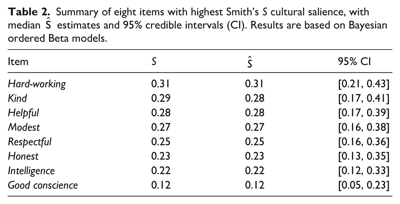
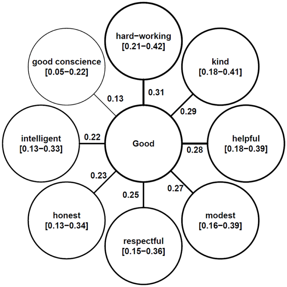
In addition to numerical tabular results, we can present this uncertainty graphically. We could use “flower plots” (often used for summarizing free-list cultural salience data), with the uncertainty intervals displayed in the text of the “petals” (Figure 1). Alternatively, we could plot the posterior distributions of $\hat{S}$ estimates for the most salient items, as seen in Figure 2.

Figure 1.

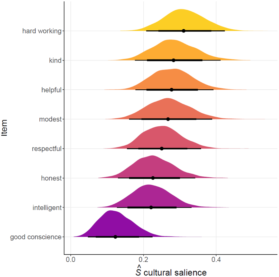
Flower plot of $\hat{S}$ estimates across the most salient item types, with 95% credible intervals displayed in the petals. Results are based on Bayesian ordered Beta models.

Figure 2.

Posterior probabilities with 95% (thin) and 80% (thick) credible intervals of $\hat{S}$ estimates across the most salient item types. Results are based on Bayesian ordered Beta models.

Regardless of the presentation method, we can thus say, for instance, that hard-working is more likely to be listed sooner and more often than good conscience as the bulk of their probability masses do not overlap. We might even suggest that these seven most salient items constitute the core cultural model here by virtue of a strong overlap in the cultural salience intervals across these item types.

Comparison across Items

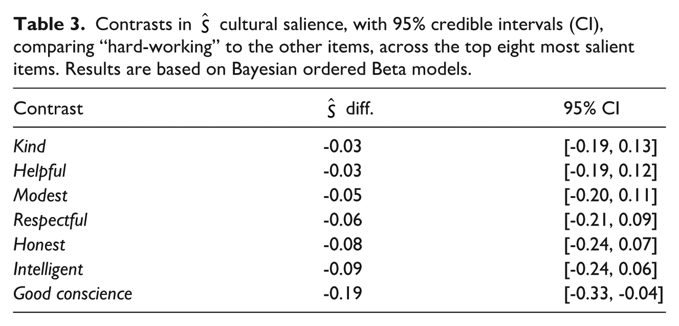
The above is definitely an improvement over ignoring uncertainty intervals but still leaves comparisons of cultural salience between items somewhat subjective. A simple extension to the method above would allow us to model these differences more formally. In other words, rather than simply presenting the predicted $\hat{S}$ estimates for each item’s posterior sample, we can compare the difference in $\hat{S}$ estimates between the items’ posterior samples.

Say we wanted to assess whether hardworking differed in cultural salience from the other items. Results of this with 95% credible intervals are shown in Table 3 (again focusing on ordered Beta models, with bootstrap and ZOIB contrasts in Supplementary Table S2), with the full distributions of contrasts summarized in Supplementary Figure S3. Based on these results, despite differences in $\hat{S}$ of nearly 0.1, the evidence that hard-working is more culturally salient than any of the other top items here largely ranges from little-to-none (e.g., for kind and helpful) to ambiguous (e.g., for honest and intelligent). For instance, intelligent is, on average, 0.09 units less culturally salient than hard-working and the bulk of the probability distribution is below 0, yet the 95% credible intervals include 0 [-0.24, 0.06]. One clearer-cut example is good conscience. With a difference in $\hat{S}$ = −0.19, 95% CI = [−0.33, −0.04], we can say that it is consistently less culturally salient than hard-working.

Table 3.

Contrasts in $\hat{S}$ cultural salience, with 95% credible intervals (CI), comparing “hard-working” to the other items, across the top eight most salient items. Results are based on Bayesian ordered Beta models.

Contrast	$\hat{S}$ diff.	95% CI
Kind	-0.03	[-0.19, 0.13]
Helpful	-0.03	[-0.19, 0.12]
Modest	-0.05	[-0.20, 0.11]
Respectful	-0.06	[-0.21, 0.09]
Honest	-0.08	[-0.24, 0.07]
Intelligent	-0.09	[-0.24, 0.06]
Good conscience	-0.19	[-0.33, -0.04]

Comparisons across Groups

In this section, we compare whether Smith’s S differs across groups. This can be done one of two ways: (1) using the intercept-only (or bootstrapping) approach above, split by group; or (2) including the group as a covariate in a regression framework. As the latter approach is more flexible (e.g., we can incorporate continuous predictors, not just categorical ones), this is the approach we focus on here (both approaches are demonstrated in the companion code).

As an illustrative example, we explore whether Tyvan good character traits differ by sex (n = 84; males = 33), focusing on kindness. From previous research, we know that this does differ (Purzycki and Bendixen 2020), with its cultural salience higher among female Tyvans ( $S_{m a l e s}$ = 0.14; $S_{f e m a l e s}$ = 0.39); women were more likely to list kindness first, and males more likely to not list kindness at all (Supplementary Figure S4).

The companion code and preprint (Major-Smith and Purzycki 2025) demonstrate how to include sex as a predictor variable in an ordered Beta model (it is easy to adapt this to a ZOIB model). Based on this model, the median $\hat{S}$ kindness value for females is 0.38, 95% CI = [0.22, 0.55], while for males it is 0.14, 95% CI = [0.03, 0.32]. The median difference between male and female $\hat{S}$ estimates is −0.24, 95% CI = [−0.45, −0.02], providing convincing evidence for a difference in the overall cultural salience of kindness as a positive character trait between the sexes in Tyvan society. On the ratio scale, kindness is approximately two-thirds less culturally salient among males compared to females $\hat{S}$ ratio difference = 0.36, 95% CI = [0.07, 0.95]).

Discussion

Researchers using free-list data in any way beyond describing the sample and data should consider calculating uncertainty, particularly for cultural salience estimates. Otherwise, they run the risk of getting a misleading picture of what people think. This article has shown a range of methods to do this, all of which give broadly similar results. Importantly, these tools facilitate bringing free-list data into a greater predictive, generative, and/or explanatory statistical framework (Purzycki 2025). While some of these models may appear rather complicated, we hope that this introduction—in conjunction with the companion code and the availability of associated software—will help encourage their use going forward.

We believe that the methods detailed in this article will greatly strengthen research using free-list data. However, they are not a panacea and there are a number of open avenues for further research. First, the focus here has been on Smith’s S cultural salience; while the overall approach of incorporating uncertainty into group-level estimates will be similar, this approach needs to be explored and extended to other useful metrics for free-list data analysis and beyond. We provide two examples of this in the companion code, first for calculating Jaccard’s similarity and conceptual overlap between domains, and second for cultural $F_{S T}$ (Bell et al. 2009) to estimate the proportion of variance in cultural traits between versus within groups.

Second, this approach of modeling uncertainty in group-level estimates can be extended beyond the simple demonstrations here when conducting cross-cultural work. For instance, researchers could incorporate this group-level uncertainty in cultural salience as a predictor in regression models (for similar approaches, see Koster et al. 2016; Purzycki 2025; Purzycki et al. 2018).

Third, as described in the introduction, a key benefit of Bayesian approaches is the ability to incorporate our prior knowledge (i.e., priors) into our models. However, throughout this article we have predominantly focused on default weakly-informative priors for simplicity. While these often suffice, they may not do so in all circumstances (especially for more complex models), and if researchers have strong background information, this knowledge ought to be used (for guidance on selecting, testing, and exploring priors, see Gelman et al. 2017; Lemoine 2019; McElreath 2020).

Finally, we modeled cultural salience for each item independently. This overlooks the reality that a change in the ordering of kindness (say) will impact the item salience—and hence cultural salience—of other free-list items. Although a more principled approach, it is much more conceptually and computationally demanding but it may be an area to explore in the future (e.g., modeling each person’s original free-list data, including the items, order, and number of items listed, then deriving item salience and cultural salience from this, factoring in the uncertainty throughout the entire process). A further future development could entail modeling uncertainty of item co-occurrence (e.g., a la social network analysis; Borgatti et al. 2018) to understand the conceptual relationships between cultural items (see Purzycki 2025).

In sum, we strongly encourage researchers using free-list data to include uncertainty estimates in their studies. This will improve the kinds of inferences we can draw about human cultural models. We hope approaches such as those demonstrated here encourage researchers to incorporate uncertainty when analyzing free-list data as a matter of course, as well as develop future extensions to the approach outlined here.

Supplemental Material

sj-docx-1-fmx-10.1177_1525822X251379224 – Supplemental material for Modeling Uncertainty around Free-list Cultural Salience Scores

Supplemental material, sj-docx-1-fmx-10.1177_1525822X251379224 for Modeling Uncertainty around Free-list Cultural Salience Scores by Daniel Major-Smith and Benjamin Grant Purzycki in Field Methods

Footnotes

ORCID iDs

Daniel Major-Smith

Benjamin Grant Purzycki

Ethical Considerations

This submission only uses previously collected, openly available data.

Consent for Publication

Not applicable.

Author Contributions

Both DM-S and BGP contributed to all stages of this submission, including conceptualizing, analysis, visualization, project management, and writing/revising.

Funding

The authors disclosed receipt of the following financial support for the research, authorship, and/or publication of this article: This project was made possible by a grant from the Templeton Religion Trust (#TRT-2022-31107). DM-S is also supported by the John Templeton Foundation (grant ref 61917).

Declaration of Conflicting Interests

The authors declared no potential conflicts of interest with respect to the research, authorship, and/or publication of this article.

Data Availability Statement

All analysis code and datasets are openly available on the following GitHub page: .

Supplemental Material

Supplemental material for this article is available online.

References

Bell

A. V.

Richerson

P. J.

McElreath

2009. Culture rather than genes provides greater scope for the evolution of large-scale human prosociality. Proceedings of the National Academy of Sciences 106:17671–74.

Bendixen

Purzycki

B. Grant

. 2025. Cognitive and cultural models in psychological science: A tutorial on modeling free-list data as a dependent variable in Bayesian regression. Psychological Methods 30:223–39.

Borgatti

S. P.

Everett

M. G.

Johnson

J. C.

2018. Analyzing social networks. London: Sage.

Boyd

Richerson

P. J.

1988. Culture and the evolutionary process. Chicago: University of Chicago Press.

D’Andrade

R. G.

1981. The cultural part of cognition. Cognitive Science 5:179–95.

Efron

Tibshirani

R. J.

1994. An introduction to the bootstrap. London: Chapman and Hall/CRC.

Gelman

Greenland

2019. Are confidence intervals better termed “uncertainty intervals”? BMJ 366: l5381.

Gelman

Hill

Vehtari

2020. Regression and other stories. Cambridge: Cambridge University Press.

Gelman

Simpson

Betancourt

2017. The prior can often only be understood in the context of the likelihood. Entropy 19:1–13.

10.

Koster

Bruno

Burns

J. L.

2016. Wisdom of the elders? Ethnobiological knowledge across the lifespan. Current Anthropology 57:113–21.

11.

Kubinec

2022. Ordered beta regression: A parsimonious, well-fitting model for continuous data with lower and upper bounds. Political Analysis 31:519–36.

12.

Lemoine

N. P.

2019. Moving beyond noninformative priors: Why and how to choose weakly informative priors in Bayesian analyses. Oikos 128:912–28.

13.

Liu

Chuen Yuen

L.-C.

Tian

G.-L.

2020. Zero-one-inflated simplex regression models for the analysis of continuous proportion data. Statistics and Its Interface 13:193–208.

14.

Major-Smith

Purzycki

B. G.

2025. Modelling uncertainty around free-list cultural salience scores. OSF Preprints. doi:10.31219/osf.io/k5ef4_v1.

15.

McElreath

2020. Statistical rethinking: A Bayesian course with examples in R and STAN. 2nd ed. Boca Raton, FL: Chapman & Hall/CRC.

16.

Ospina

Ferrari

S. L. P.

2012. A general class of zero-or-one inflated beta regression models. Computational Statistics and Data Analysis 56:1609–23.

17.

Purzycki

B. G.

2025. Ethnographic free-list data: Management and analysis with examples in R. London: Sage.

18.

Purzycki

B. G.

Bendixen

2020. Examining values, virtues, and tradition in the republic of Tuva with free-list and demographic data. The New Research of Tuva 4:6–18.

19.

Purzycki

B. G.

Jamieson-Lane

2017. AnthroTools: An R package for cross-cultural ethnographic data analysis. Cross-Cultural Research 51:51–74.

20.

Purzycki

B. G.

Pisor

A. C.

Apicella

Atkinson

Cohen

, et al. 2018. The cognitive and cultural foundations of moral behavior. Evolution and Human Behavior 39:490–501.

21.

Purzycki

B. G.

Stagnaro

M. N.

Sasaki

2020. Breaches of trust change the content and structure of religious appeals. Journal for the Study of Religion, Nature and Culture 14:71–94.

22.

Quinlan

M. B.

2005. Considerations for collecting freelists in the field: Examples from ethnobotany. Field Methods 17:219–34.

23.

R Core Team. 2023. R: A language and environment for statistical computing. Vienna, Austria: R Foundation for Statistical Computing.

24.

Robbins

M. C.

Nolan

J. M.

2019. Free-list measures of cognitive sharing and organization: Ethnobotany in rural Missouri. Field Methods 31:167–80.

25.

Robbins

M. C.

Nolan

J. M.

Chen

2017. An improved measure of cognitive salience in free listing tasks: A Marshallese example. Field Methods 29:395–403.

26.

Smith

J. J.

Borgatti

S. P.

1997. Salience counts-and so does accuracy: Correcting and updating a measure for free-list-item salience. Journal of Linguistic Anthropology 7:208–9.

27.

Sperber

1996. Explaining culture: A naturalistic approach. Malden, MA: Blackwell.

28.

Sutrop

2001. List task and a cognitive salience index. Field Methods 13:263–76.

Supplementary Material

Please find the following supplemental material available below.

For Open Access articles published under a Creative Commons License, all supplemental material carries the same license as the article it is associated with.

For non-Open Access articles published, all supplemental material carries a non-exclusive license, and permission requests for re-use of supplemental material or any part of supplemental material shall be sent directly to the copyright owner as specified in the copyright notice associated with the article.

0.00 MB

0.11 MB