Sage Journals: Discover world-class research

Abstract

Using data from the states’ annual comprehensive financial reports for the period 2003 to 2018, the authors apply a dynamic panel model frame to test how state tax and expenditure limitations (TELs) and rainy-day funds (RDFs) affect key aspects of the state fiscal condition. Guided by the fiscal illusion theory, we hypothesize that TELs and RDFs will affect various short-term solvency indicators but will not have a significant impact on pension and long-term solvency indicators. The study provides mixed empirical evidence, cautioning that these relations are complex. The results provide empirical evidence supporting most of the hypotheses related to short-term solvencies, such as cash and budgetary solvencies. In addition, the study finds that neither tax nor expenditure limitations have a significant impact on the net asset ratio and the long-term ratios. Similarly, there is evidence that TELs and RDFs do not affect the two pension solvency ratios. This is probably the first study to provide a dynamic panel model to assess how two major state fiscal institutions influence various state government’s short-term and long-term fiscal solvency conditions.

Keywords

financial condition evaluation tax and expenditure limitations rainy-day funds

State budgetary and financial conditions are affected by state fiscal policies such as tax and expenditure limitations (TELs) and rainy-day funds (RDFs). These policies have different policy goals: TELs have been introduced to reduce government spending by limiting tax increases and reducing spending, while RDFs have been used to strengthen the borrowing position of the government and provide a cushion during financial hardship. Arguably, both instruments could improve the financial position of the government. We, however, argue that the relations are more complex. We contend that the combination of these policies may have different impacts on the short-term and the long-term state financial condition indicators.

We apply the fiscal illusion lenses to derive our hypotheses regarding the intricate relations of tax and expenditure limits and RDFs with the state government’s financial position in the short term and the long term. The fiscal illusion theory postulates that citizens’ perceptions of government spending are obscured by the way governments collect revenues and spend the resources. The more covert the methods of spending, the bigger the citizens’ misperception. Following this premise, a state government will conform to TELs rules by not increasing revenues in highly transparent categories, such as the ones used to calculate cash, budget, and service solvency indicators, while finding and employing “hidden” ways, such as increasing debt funding and/or reducing pension funding. With regards to RDFs, fiscal illusion theory could be applied in a way that RDFs would be expected to worsen short-term fiscal health while having no significant impact on long-term fiscal health.

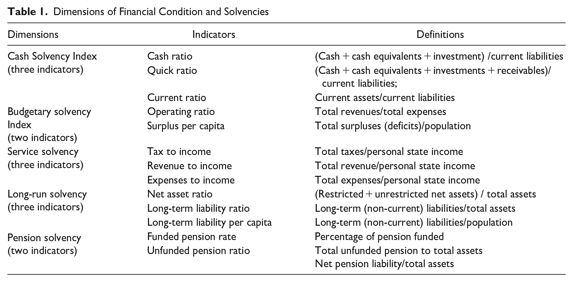
The analytical tools to assess governmental financial condition have evolved over the past two decades. While there is no consensus as to which ones are the best, there are a set of indicators to measure state financial condition that have consistently been used to assess the condition of state finances (Yan & Carr, 2019). One way to measure financial condition is by using multiple financial ratios to assess the financial condition of the studied government entities. Financial ratios, according to the literature, measure several key aspects of solvency, most notably, cash solvency, budgetary solvency, service solvency, and long-run solvency (Arnett, 2014; Singla & Stone, 2018; Stone et al., 2015; Wang et al., 2007). This study identifies a set of financial indicators and ratios for assessing the fiscal condition and utilizes annual comprehensive financial report (ACFR) data for the period 2003 to 2018 to examine the financial performance of state governments. We run dynamic models on commonly used ratios for cash, budgetary, service, long-term, and pension solvencies (please see Table 1 for all solvency ratios and the formulas we use to calculate them). Using a modified analytical framework, we examine a selected number of policies and socioeconomic factors that are related to the state’s financial condition. The central policy variables of interest are states’ TELs, which are disaggregated into tax limitations and expenditure limitations, and states’ RDFs. Moreover, this research attempts to disentangle the factors that influence states’ fiscal condition. Most of all, we are concerned with the degree to which TELs and states’ RDFs affect the solvency indicators. Second, the research examines whether these factors have contrasting associations with short-term solvencies and long-term solvencies, respectively, by applying the fiscal illusion theory.

Table 1.

Dimensions of Financial Condition and Solvencies

Dimensions	Indicators	Definitions
Cash Solvency Index (three indicators)	Cash ratio	(Cash + cash equivalents + investment) /current liabilities
	Quick ratio	(Cash + cash equivalents + investments + receivables)/current liabilities;
	Current ratio	Current assets/current liabilities
Budgetary solvency Index (two indicators)	Operating ratio	Total revenues/total expenses
Budgetary solvency Index (two indicators)	Surplus per capita	Total surpluses (deficits)/population
Service solvency (three indicators)	Tax to income	Total taxes/personal state income
	Revenue to income	Total revenue/personal state income
	Expenses to income	Total expenses/personal state income
Long-run solvency (three indicators)	Net asset ratio	(Restricted + unrestricted net assets) / total assets
	Long-term liability ratio	Long-term (non-current) liabilities/total assets
	Long-term liability per capita	Long-term (non-current) liabilities/population
Pension solvency (two indicators)	Funded pension rate	Percentage of pension funded
Pension solvency (two indicators)	Unfunded pension ratio	Total unfunded pension to total assets Net pension liability/total assets

In the next section, we review relevant literature on TELs, RDFs, and financial condition evaluation. Then, we introduce the data and models used to evaluate the financial condition and hypothesis testing on the variables of interest, including tax limitations, expenditure limitations, and RDFs. It is followed by the results from the data analysis and discussions of the results. The final part summarizes the key findings, discusses the research limitations, and makes suggestions for further studies.

Literature Review

Tax and Expenditure Limits

Various forms of tax and expenditure limits, adopted by state governments in response to increased tax burdens and government growth, have been one of the major state fiscal policies over the past half-century in the United States. State lawmakers, conservative and liberal states alike, took measures to link the growth in revenues or expenditures to economic conditions, especially during the 1970s and 1980s. The most notable event on TELs is California’s Proposition 13 which was passed in 1978. Since then, TELs gained increased popularity in the U.S. in the 1970s through 1990s, of which Massachusetts Proposition 2½ in 1980 and Colorado’s Taxpayer Bills of Rights in 1992 are among the most well-known ones (Amiel et al., 2009; Mullins & Joyce, 1996; Stallmann et. al., 2017).

The proliferation of TELs engendered a good number of studies that examined the content of TELs, the factors that motivated states’ adoption of various TELs from one side (Miller et al., 2005), as well as the effect of TELs on state government budget behaviors, including revenues, expenditures, and other aspects of budget conditions on the other side (Amiel et al., 2009; Bae et al., 2012; Ermasova & Kulik, 2018; Mullins & Joyce, 1996; Mullins & Wallin, 2004). In terms of the contents of TELs, Amiel et al., (2009) analyzed the detailed requirements of TELs and developed an index to measure the restrictiveness of the state TELs, which have been utilized by some subsequent studies on TELs. On the impacts of TELs, early studies find that TELs have a profound influence on the revenue structure of both state and local governments and their ability to respond to the increased demands and citizen preferences (Mullins & Joyce, 1996). Similarly, TELs are also found to be effective in reducing government revenues (Skidmore, 1999) and in curbing government growth (Seljan, 2014). However, Bae et al. (2012) found that there was little or no impact of TELs on state expenditures. Maher et al. (2017) also found that the impact of TELs on state fiscal reserves is marginal or weak, whereas Amiel et al. (2014) found that there were varied impacts on revenues and expenditures.

TELs may affect financial conditions and other budgetary conditions as well. Jimenez (2018) investigates the impact of local TELs on municipal budgetary solvency and claims that TELs, at least at a local level, do not take into consideration possible changes in voters’ preferences or even future fiscal shocks, thus reducing government’s flexibility to act accordingly during crisis. Lacking flexibility, TELs negatively impact budget solvency (Jimenez, 2018). As part of TELs, specific legislative rules on tax and revenues alone may affect budget conditions. Lee (2014) finds that the magnitude of the effect of supermajority rule on tax burden diminished over time. In a later study, Lee (2018) finds that the most stringent state rule proves ineffective in controlling states’ budget expansion. The author concludes that, at best, the supermajority rule for tax increases may have limited effect in the short term, but this effect decreases in the long run. Maher and Deller (2010), in their study of municipal government, find that TELs are associated with several financial indicators on revenue and expenditure capacity, fund balance and debt service, general obligation debt, pension funding, and operating position. However, such a relationship is yet to be examined by the state government. Overall, relevant studies focused on TELs find mixed evidence regarding their influence over variables affecting state or local financial conditions.

The fiscal illusion theory may provide an explanation of the effect of TELs on state governments’ short-term and long-term fiscal health. The underlying premise of the fiscal illusion theory is that citizens’ misperceptions of the true tax burden and government services could change the fiscal behavior of the government in terms of where and how funds get allocated and spent (Buchanan & Wagner, 1977). The public choice theory posits that bureaucrats, as rational actors, serve their interests and are budget maximizers (Niskanen, 1971, 1994; Tempelman, 2007). The government as an agent and the taxpayers as principals have a relationship characterized by imperfect information flowing from the agent to the principal (Seljan, 2014). In a perfect world, the principal will make rational decisions; however, given the limited information, taxpayers tend to have better knowledge and control over the most transparent aspects of government finances, such as cash, service, and operating solvencies. Therefore, according to the proponents of fiscal illusion theory, governments tend to increase spending on some categories, such as debt and pension obligation (Hoang & Maher, 2022).

In the context of TELs, the fiscal illusion premise manifests its effect when voters opt to support debt financing to reduce increases in current tax payments when they do not possess full information on future debt and its consequences. Some studies found that countries with high levels of debt are associated with a high degree of fiscal illusion (Dell’Anno & Dollery, 2014), and the US government is not an exception (Boccia, 2022). However, there has been rather limited research on the impact of TELs on state financial conditions. A recent study by Hoang and Maher (2022) found that state pension contribution is negatively associated with budgetary fund balances, total reserve fund balances, and state expenditures, providing some evidence that state government prioritized short-term operational spending over long-term fiscal conditions. However, it is yet to examine the overall impact of TELs on state financial conditions. Furthermore, the tax limitations and expenditure limitations may, in fact, have contrasting influences on various short-term solvency indicators.

Hypothesis 1a: The stringency of tax limitations is negatively associated with highly visible short-term solvency indicators, whereas expenditure limitations are positively associated with these indicators.

Hypothesis 1b: Neither tax limitations nor expenditure limitations are significantly associated with less visible categories such as long-term debt and pension solvency indicators. The one exception is per capita long-term debt, which is expected to be improved by both institutions due to its transparency with the public.

Rainy-Day Funds

Another variable of interest in measuring states’ fiscal solvency is the amount of states’ budget reserve funds. Budget reserves, or budget stabilization funds (BSFs), which in this paper are interchangeably referred to as rainy-day funds (RDFs), are intended to alleviate the budget deficits caused by economic downturns or unexpected spending (Tax Policy Center, 2020). The role of these funds is countercyclical, stabilizing budget fluctuations, particularly during recessions (Ryu et al., 2020). Most of the states set a cap on fund balances and stipulate how the excess balance shall be allocated. All states have established BSFs or similar funds under different names. It is found that the level of rainy-day funds has been restored and increased to a higher level since after the Great Recession, averaging about 12% of general fund balances in 2023 (NASBO, 2023). Prior studies have found that BSFs are more effective in stabilizing budget fluctuations during recessions than general fund balances. BSFs are, therefore, more effective in reducing cyclical fiscal stress. For example, Wagner (2003), in his examination of states’ reserves, finds that they improve a state’s fiscal and overall economic performance during a crisis. Similarly, Hou (2005) finds that states’ fiscal reserves and own revenues also played a critical role in closing state expenditure gaps during fiscal crises. A study by Wei and Denison (2019) finds that RDFs were effective in stabilizing general fund expenditures during both recessions and economic expansions. More recently, Ryu et al. (2020) found empirical evidence of the political manipulation of states’ reserve funds just before elections. More specifically, the authors find that both general fund balances and BSFs declined before and during election years and increased in the year following elections. This pattern is even more salient in states with more stringent tax expenditure limitations.

The relationship between TELs and RDFs is complex. Theoretically, effective TELs can improve financial conditions by limiting government growth and increasing efficiency and accountability. On one hand, TELs may constrain the options of raising taxes and, hence, the ability of the state government to respond to budget shortfalls or fiscal distress. However, increasing the level of fiscal reserve increases the state government’s capacity to respond to fiscal stress caused by economic downturns. Furthermore, stringent TELs may constrain the amount of funds set aside for fiscal reserve and hence the state government’s capacity to respond to budget shortfalls. Hou (2003, 2005) argues that TELs positively affect a state’s fiscal reserves. However, Maher et al. (2017) did not find strong evidence to support this claim.

Following the underlying fiscal illusion premise, RDFs will reduce visible spending in favor of increased reserves. Higher reserves could improve the overall service delivery, while negatively impacting cash and budgetary solvencies. When it comes to long-term solvencies, it could be argued that pressure for higher reserves could increase long-term debt financing and pension underfunding. However, higher reserves could also impact the government’s credit rating, thus pushing for lower debts and better long-term solvency. These competing forces could result in an overall statistically insignificant relation between RDFs and long-term solvency. Thus, we propose the following hypotheses:

Hypothesis 2a: Rainy-day funds are positively related to service solvency indicators but negatively related to cash and budgetary solvency indicators.

Hypothesis 2b: Rainy-day funds do not have a statistically significant relationship with either long-term debt or pension solvency indicators. The only exception is per capita long-term debt, which is expected to be improved by both fiscal institutions due to its transparency with the public.

Evaluating Financial Condition

The importance of measuring and evaluating fiscal performance at state and local levels is well established in the public administration and public budgeting literature mainly because it is one of the core components of public sector accountability (Cabaleiro et al, 2013; Clark, 2015; Maher et al, 2023; Rivenbark et al, 2010; Wang, et al, 2007). As a financial management tool, measuring governmental financial performance could serve as an early warning system to signal financial difficulty and, potentially, to prevent major disruptions in the provision of critical government services. Financial performance is critical for every organization because it determines its ability to continue its operations. Government organizations’ financial performance assumes an additional function, namely, accountability of governments to serve their constituents.

There have been several different models developed for measuring the fiscal health of state and local governments. However, the vast majority of these models are intended for local government. For instance, two of the models—the Financial Trend Monitoring System (FTMS) promoted by the International City and County Management Association and the 10-point test of financial condition developed by Ken Brown, are well-known (Groves & Valente, 1986; Nollenberger et al., 2003). Subsequent efforts have been made to these models (Maher & Deller, 2011; Maher et al, 2023; Maher & Nollenberger, 2009). While these models are relevant, they have limited applicability to state governments because local governments’ revenue and expenditure structures, as well as their political systems, are distinctly different from state governments. In contrast, the model developed by Wang et al. (2007) for evaluating state government is more relevant. The model constructs a comprehensive financial condition index by incorporating four financial condition dimensions, namely, cash, budget, long-run, and service-level solvencies. These dimensions were built on 11 financial ratios that included information about states’ cash, liabilities, assets, taxes, revenues, expenses, and debt. Furthermore, they also used many demographic and socioeconomic indicators to test the measures’ relevance and validity. This model offers some key insights into the variables beyond fiscal indicators. However, their analysis was based on the observation from only one single fiscal year, which poses a serious limitation. Arnett (2014) applied Wang’s 4-dimensional model to evaluate and ranked state financial condition by assigning different weights to each of the 11 financial ratios. Norcross and Gonzalez (2018) at the Mercatus Center advanced Wang’s model by adding trust fund solvency to account for obligations from pension and other post-employment benefits. They also modified measures for service solvency by calculating it as a ratio of taxes, revenues, and expenses to state individual income as opposed to the more traditional calculation of per capita ratios. More recently, Shi (2020) applied ambiguous logic to evaluate and rank state financial conditions during the Great Recession based on Wang’s model and the subsequently modified models.

It is noteworthy that while many academic studies measure financial performance, there is little agreement regarding the most relevant dimensions (Kioko, 2013). Therefore, the use of indicators is not consistent across studies. This is to be expected (and justified), at least to some level, because the choice of specific indicators depends on the topic of an academic study and the needs it tries to meet. Some authors, however, have recognized that the indicators used in academic studies do not necessarily correspond with the indicators commonly used by practitioners in government accounting and finance (Maher, 2013; Maher & Deller, 2011). Gorina et al. (2017) also point out that calculating fiscal indicators and other environmental variables should be geared toward predicting fiscal crises. Measuring financial performance, therefore, has become more relevant from both a theoretical perspective and as a tool for practitioners. In sum, we generally expect a state’s financial condition to be evaluated comprehensively in several key different dimensions of solvency by using long-term and short-term solvency indicators.

Data and Methodology

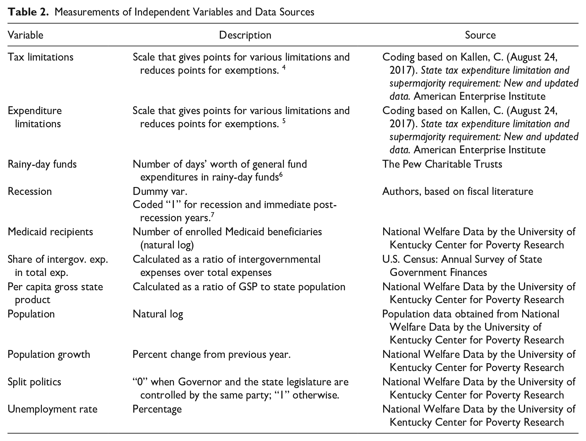
The dataset used in this study, which includes financial, demographic, policy, economic data, and data on state politics, was obtained from multiple sources. The financial data include state ACFR data for 2003 to 2018, of which the data for 2006 to 2016 was obtained from Norcross and Gonzalez (2018),¹ and for the period 2003 to 2005 and 2017 to 18 was extracted from the states’ ACFRs by the authors. Other fiscal data on operating revenues, expenses, and budget balances were from the U.S. Census Annual Survey of State Government Finances. For the data on fiscal policy, we use the stringency index of state tax expenditure limitations developed by Amiel et al. (2014)² and updated by Kallen (2017). Using the method described in Kallen (2017) and reviewing individual state’s changes for the period thereafter, we separated the TELs into two categories—tax limits and expenditure limits, to examine their disparate effect on financial condition. Data on RDFs, the net pension liabilities, and the funded pension ratio were from the Pew Charitable Trusts (PCT)³. PCT measures RDFs in the number of days the fund can support the operation. The RDF amount includes all reserves and statutory and current balances and is compared to a day of expenses needed to sustain a state’s government operations. Finally, the data for Medicaid recipients, population, unemployment rate, and state politics come from the National Welfare Data at the University of Kentucky Center for Poverty Research. For a detailed list of data and data sources, please refer to Table 2.

Table 2.

Measurements of Independent Variables and Data Sources

Variable	Description	Source
Tax limitations	Scale that gives points for various limitations and reduces points for exemptions. ⁴	Coding based on Kallen, C. (August 24, 2017). State tax expenditure limitation and supermajority requirement: New and updated data. American Enterprise Institute
Expenditure limitations	Scale that gives points for various limitations and reduces points for exemptions. ⁵	Coding based on Kallen, C. (August 24, 2017). State tax expenditure limitation and supermajority requirement: New and updated data. American Enterprise Institute
Rainy-day funds	Number of days’ worth of general fund expenditures in rainy-day funds⁶	The Pew Charitable Trusts
Recession	Dummy var. Coded “1” for recession and immediate post-recession years.⁷	Authors, based on fiscal literature
Medicaid recipients	Number of enrolled Medicaid beneficiaries (natural log)	National Welfare Data by the University of Kentucky Center for Poverty Research
Share of intergov. exp. in total exp.	Calculated as a ratio of intergovernmental expenses over total expenses	U.S. Census: Annual Survey of State Government Finances
Per capita gross state product	Calculated as a ratio of GSP to state population	National Welfare Data by the University of Kentucky Center for Poverty Research
Population	Natural log	Population data obtained from National Welfare Data by the University of Kentucky Center for Poverty Research
Population growth	Percent change from previous year.	National Welfare Data by the University of Kentucky Center for Poverty Research
Split politics	“0” when Governor and the state legislature are controlled by the same party; “1” otherwise.	National Welfare Data by the University of Kentucky Center for Poverty Research
Unemployment rate	Percentage	National Welfare Data by the University of Kentucky Center for Poverty Research

Dependent Variables

As noted in the literature review, using multiple financial ratios is one of the main approaches to the measurement of the financial condition (Arnett, 2014; Singla & Stone, 2018; Stone et al., 2015; Wang et al, 2007). These financial ratios measure several key aspects of solvency, including cash, budgetary, service, long-run, and pension solvencies. This study identifies a set of financial indicators and ratios for state governments as dependent variables. In our construction of solvency indexes, we standardize these ratios and run Cronbach’s alpha tests to determine the internal consistency of the ratios that are to be included in composite indexes for cash solvency, budgetary solvency, service solvency, long-term solvency, and pension solvency. The results from Cronbach’s alpha reveal that the test scores for cash, budgetary, and service solvency are all over 0.9, indicating very strong consistency, and therefore, could be used in constructing composite solvency indexes. However, the test scales for long-term and pension solvencies are 0.5037 and 0.6179 respectively, revealing a weak consistency. Therefore, we do not use long-term composite indexes. Instead, we follow the literature and use individual long-term fiscal health indicators.

As a result, for our dependent variables, we use three ratios to measure cash solvency (cash, quick, and current ratios), two ratios for budget solvency (per capita surplus/deficit and operating ratios), three ratios for service solvency (tax to income, revenue to income, and expenditure-to-income ratios), three ratios for long-term solvency (net assets, long-term liability ratios, and per capital long-term liability), and two pension solvency ratios (unfunded pension and funded pension ratios). Table 1 provides formulas for each of the individual ratios used. In addition, we construct cash solvency, budgetary solvency, and service solvency composite indexes using the ratios earlier. Table 1 describes the ratios and dimensions we use in our analysis.

Measuring Policy and Control Variables

Regarding the main policy variables, one of the major challenges related to states’ TELs is the measurement and practical operationalization of TELs (Deller & Stallmann, 2009; Kallen, 2017; Maher et al., 2017; Mullins & Joyce, 1996). It is now widely accepted that TELs are exceedingly complicated and, therefore, cannot be measured with only one dichotomous variable. Almost every state has a different set of TELs, varying in terms of the type of TELs (revenue, expenditure, statutory, or constitutional), growth restrictions, method of approval, inclusion of override provisions, and exemptions. Therefore, many authors in the past two decades have resorted to using an index that accounts for all these factors. Kallen (2017) provides a comprehensive index that builds on the work of Amiel et al. (2009) and Amiel et al. (2014), assigning different numbers of points for each of the categories and deducting points for cases of exemptions. The maximum scale reaches 30 points, with a minimum of 0 points, allowing an adequate range to capture the various combinations of state TELs. This index has become a common measurement in most of the recent fiscal studies on TELs. We use the descriptions provided by Kallen and disaggregate TELs to tax limitations and expenditure limitations. For the period after 2016, we use the same criteria to update for any changes.

It is important to recognize that the measurement of financial condition is related to the fiscal health and fiscal sustainability of the government organization. Therefore, identifying the factors that cause fiscal stress and undermine fiscal sustainability becomes an important step in financial analysis and management. Fiscal distress has been largely attributed to four general factors: population decline and consequently reducing demand, growth of government due to disproportional increase of government spending relative to inflation and population growth, shifting demands of various interest groups, especially when elected officials are vulnerable to certain interest groups, and poor public sector management (Kloha et al., 2005, p. 315).

Given this recognition and finding, the control variables included in our analysis are the following: population growth, gross state product, number of Medicaid recipients, unemployment rate, split legislative and executive government, as well as several indicators measuring structural characteristics of revenue and expenditure. For population growth and gross state product, we expect that they are generally positively associated with both short-term and long-term financial conditions, whereas unemployment rate, proportion of Medicaid recipients, and recession are negatively associated with both short-term and long-term financial conditions, Regarding the political controls, the effect of a divided state government is undetermined as it may or may not be beneficial to long-term fiscal health due to political competition. A divided government may not necessarily be detrimental to fiscal health as political competition in the form of checks and balances may lead to more prudent financial management practices and policies. For the structure of revenue and expenditure, we expect that the share of intergovernmental expenditure is inversely related to financial condition as it is a burden to state government.

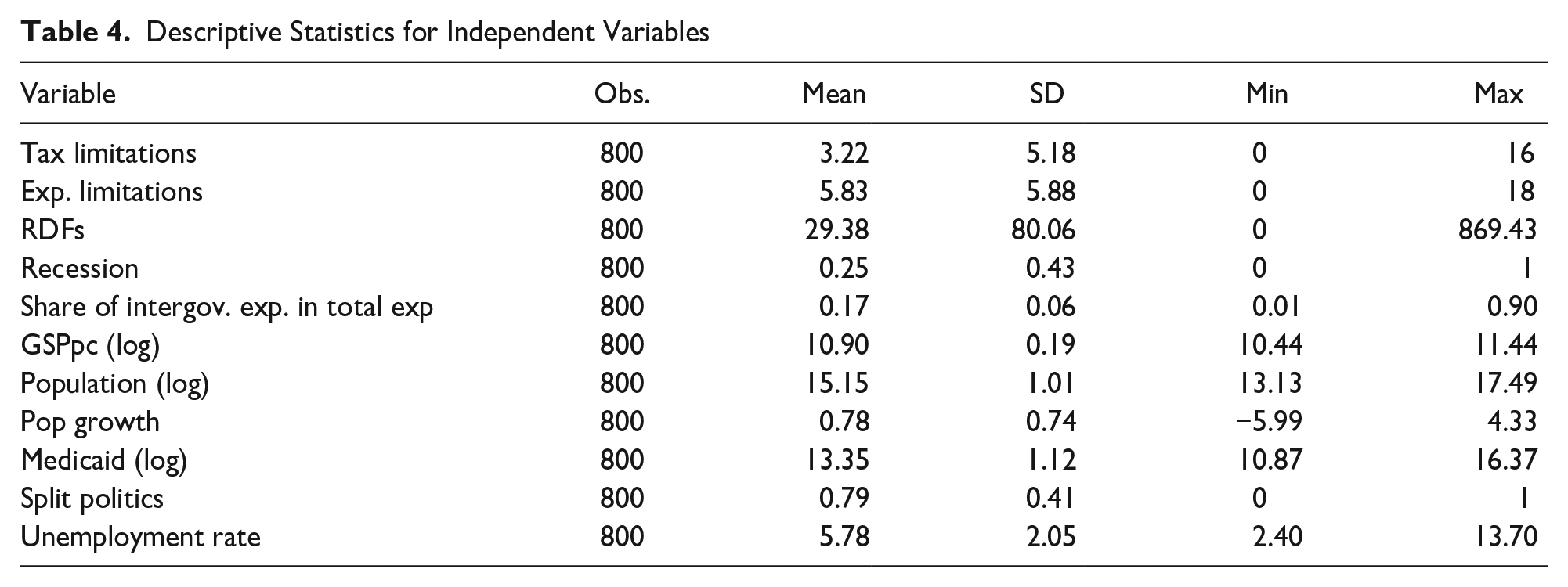
The details of variables and measurements are provided in Table 2. The descriptive statistics of dependent and independent variables are provided in Tables 3 and 4.

Table 3.

Descriptive Statistics for Dependent Variables

Variable	Obs.	Mean	SD	Min	Max
Cash ratio	800	1.96	2.27	0.03	26.84
Quick ratio	800	2.72	2.36	0.24	28.04
Current ratio	800	2.96	2.40	0.00	28.04
Surplus per capita	800	257	1,334	−10,997	15,302
Operating ratio	800	1.04	0.16	0.32	4.25
Tax to income	800	59.59	18.74	3.06	252.28
Revenue to income	800	137.58	46.35	68.08	523.61
Expenditure to income	800	132.23	34.97	36.52	297.17
Net asset ratio	800	1.04	0.16	0.32	4.25
Long-term liability ratio	800	0.42	0.53	0.01	5.49
Pension ratio	800	0.41	0.43	−0.20	3.85
Funded ratio	800	0.76	0.15	0.31	1.14
Cash solvency index	800	−8.82E–10	2.93	−3.59	18.88
Budget solvency index	800	4.03E–09	1.96	−12.72	13.11
Service solvency index	800	−4.93E–09	2.61	−7.53	9.92

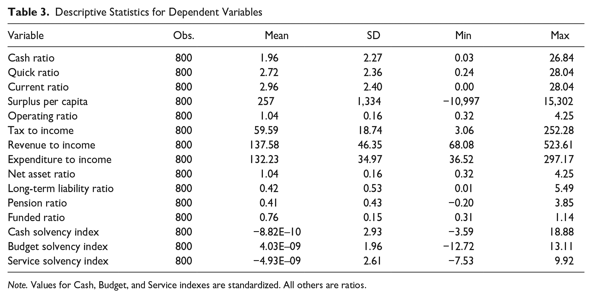
Note. Values for Cash, Budget, and Service indexes are standardized. All others are ratios.

Table 4.

Descriptive Statistics for Independent Variables

Variable	Obs.	Mean	SD	Min	Max
Tax limitations	800	3.22	5.18	0	16
Exp. limitations	800	5.83	5.88	0	18
RDFs	800	29.38	80.06	0	869.43
Recession	800	0.25	0.43	0	1
Share of intergov. exp. in total exp	800	0.17	0.06	0.01	0.90
GSPpc (log)	800	10.90	0.19	10.44	11.44
Population (log)	800	15.15	1.01	13.13	17.49
Pop growth	800	0.78	0.74	−5.99	4.33
Medicaid (log)	800	13.35	1.12	10.87	16.37
Split politics	800	0.79	0.41	0	1
Unemployment rate	800	5.78	2.05	2.40	13.70

Empirical Model

The incremental nature of the government budgets calls for the application of dynamic empirical models to examine the relationship between the state government’s fiscal health and the two major fiscal institutions, TELs and RDFs. In addition, the potential for endogeneity bias due to the correlation of the control variables with the error term could lead to incorrect results and conclusions. Finally, most economic, and financial models suffer from problems related to omitted variables, which can be difficult to measure and/or collect. In an attempt to address these challenges, we applied the Generalized Method of Moments (GMM) model, which uses the lagged dependent variable as a valid instrument. Introduced by Anderson and Hsiao in 1982 and advanced by other scholars (Arellano & Bond, 1991; Arellano & Bover, 1995; Blundell & Bond, 1998), GMM has become increasingly popular in many policy areas, especially in public finance and economics, where fiscal policy implications are typically associated with time lags. The estimators in the GMM models are designed specifically for models such as the one used in this paper, where the number of periods “t” is relatively small compared to the number of individual units (states), “n.”. Moreover, the GMM is an appropriate specification for instances when the change in the dependent variable is contingent on its past performance. GMM specifications also address the problem of control variables that may not be strictly exogenous to the error term (Roodman, 2009a, 2009b), which could be a case when using multiple budget variables. Finally, the GMM estimator arguably outperforms the fixed effect specifications because the former accounts for state-specific characteristics.

The model specification is the following:

Y i t = b 1 + δ Y i, t - 1 + β X i t + U i + ϑ i t

i = 1, 2, \dots, 50; t = 1, 2, \dots (2003 - 2018)

(1)

where Y_{i, t-1} represents the lagged dependent variables in the state “i” and year “t” for the selected financial condition measures, including both solvency indexes as well as individual ratios. The individual ratios are cash ratio, quick ratio, current ratio, surplus/deficit ratio, operating ratio, tax-to-income ratio, revenue-to-income ratio, expenditure-to-income ratio, net assets ratio, long-term liabilities ratio, per capita long-term liabilities ratio, funded pension ratio, and unfunded pension ratio, cash solvency index, budget solvency index, and service solvency index. TaxL, ExpL, and RDF represent tax limitations, expenditure limitations, and RDFs, respectively, and X_{i, t} is a vector for tax limitations, expenditure limitations, and RDFs as well as the control variables, including intergovernmental expenditure share, per capita GSP, population, population growth, Medicaid recipients, split state politics, unemployment rate, and recession.

Assuming no serial correlation, the values of the Y lagged for two or more periods can be taken as valid instruments for the transformed lagged variables $Δ Y i t$ = Y_i,t−Y_i,t-1.

Δ Y i t = \sum α Δ Y i t, t - 1 + β X^{'} i t = Δ ϑ i t

(2)

We use two lagged periods as instruments and we assume that our control variables are weakly exogenous and, as such, uncorrelated with the future realization of the error term. Following specifications by Arellano and Bover (1995) and Blundell and Bond (1998), we implemented the system GMM, incorporating a combination of the moment conditions for the difference equation and the level equations.

We report the probabilities for the Hansen-J test of over-identifying restrictions. The null hypothesis is that the instruments are exogenous, and a p-value tends to be inflated as the number of instruments increases. We collapse the instruments to avoid this increase of p-value. We also report the probabilities for the Arellano-Bond z-test for serial correlation in the residuals, which assesses the presence of the first-order serial correlation. A probability lower than the statistically significant level would suggest correlated errors. Finally, the number of instruments in all model specifications is lower than the number of units, that is, states.

Results and Discussions

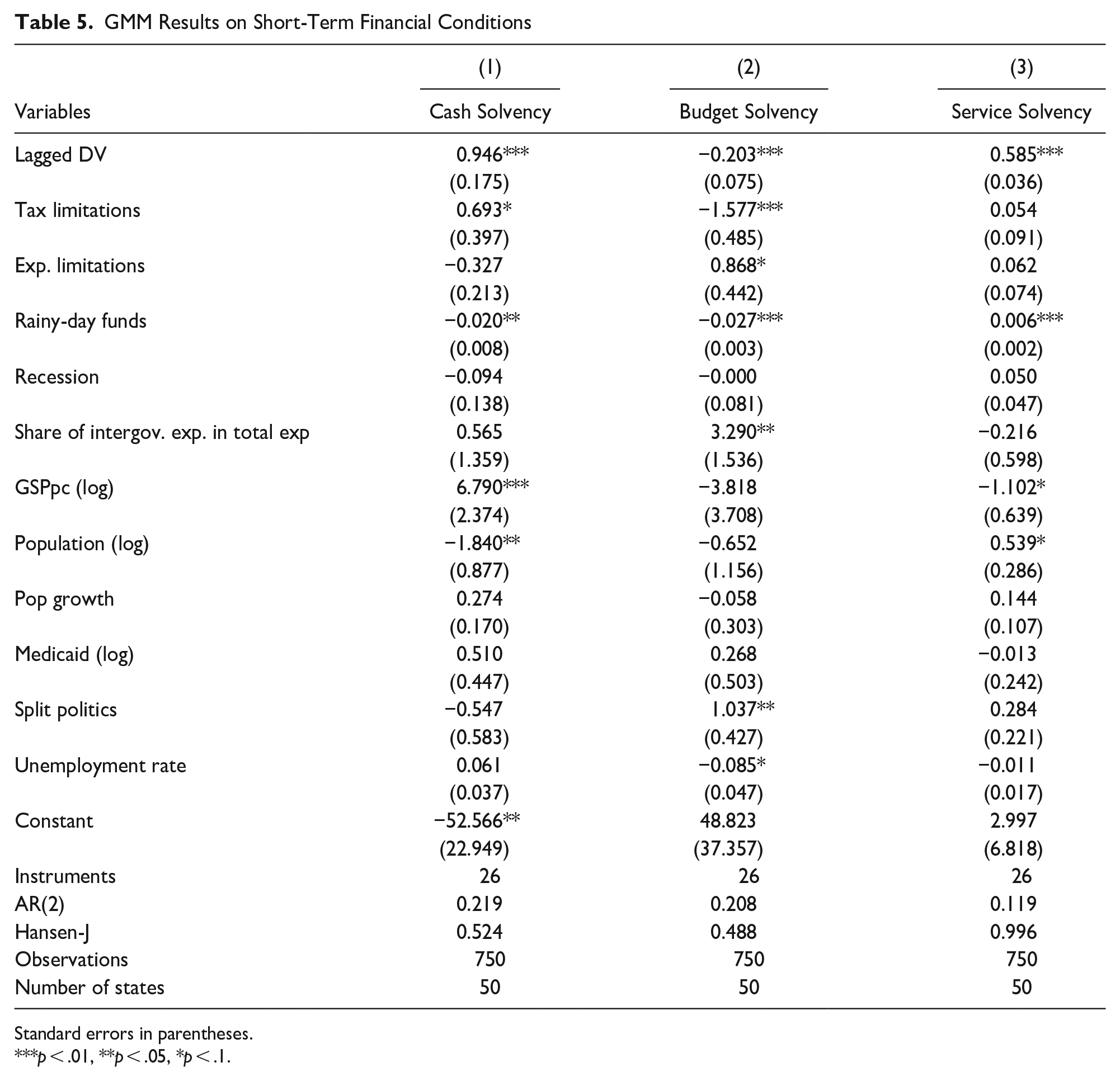
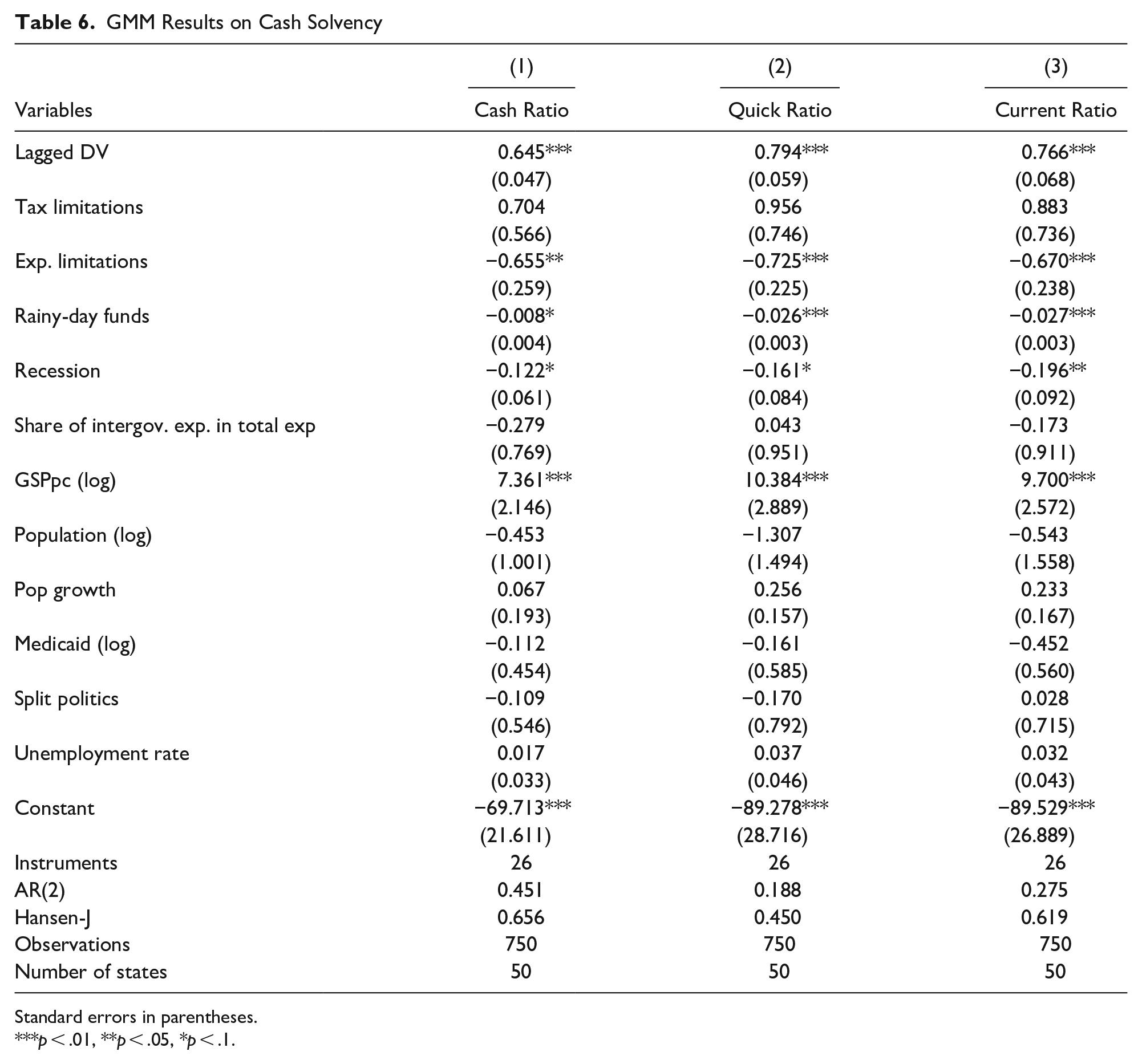
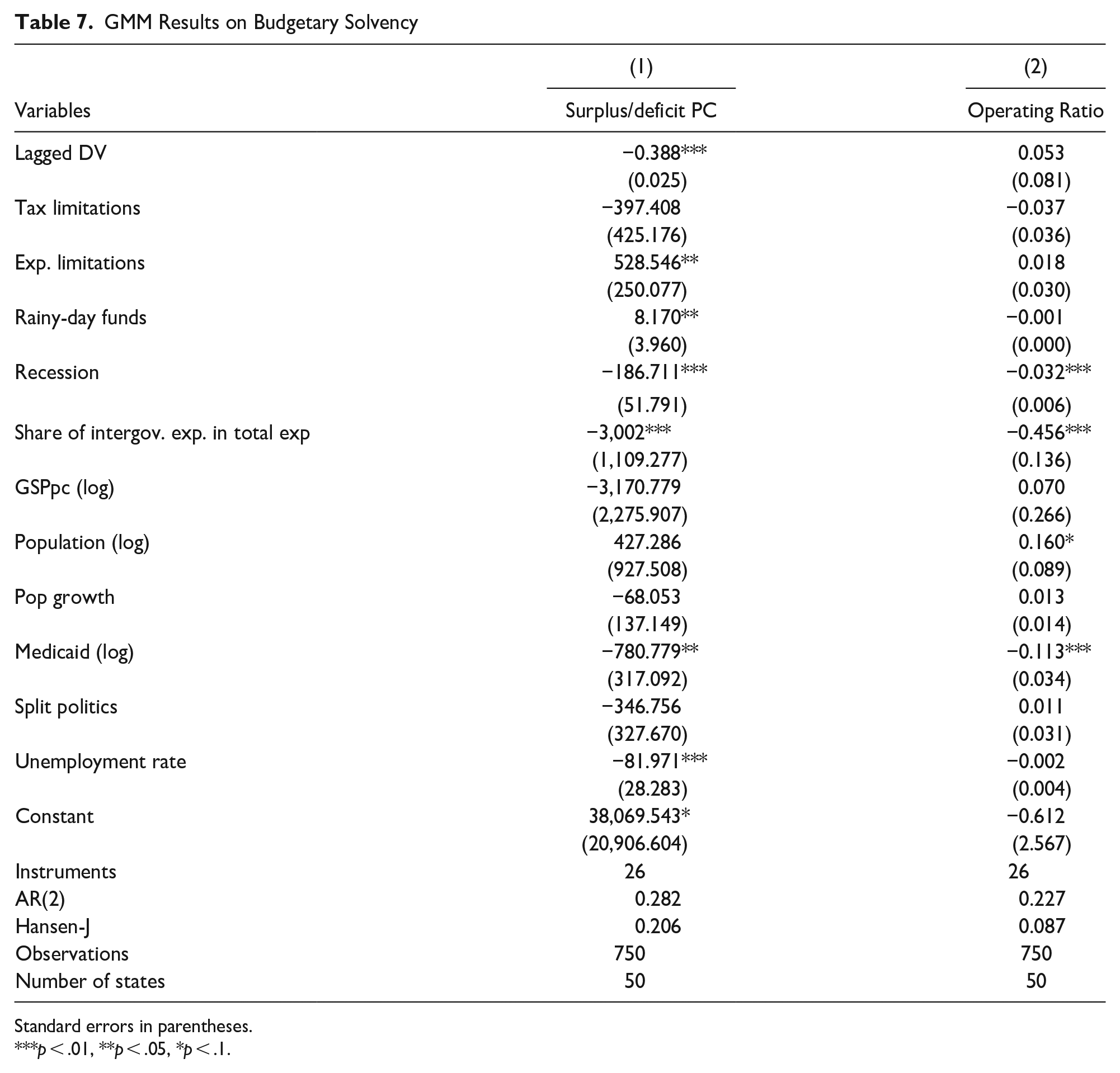
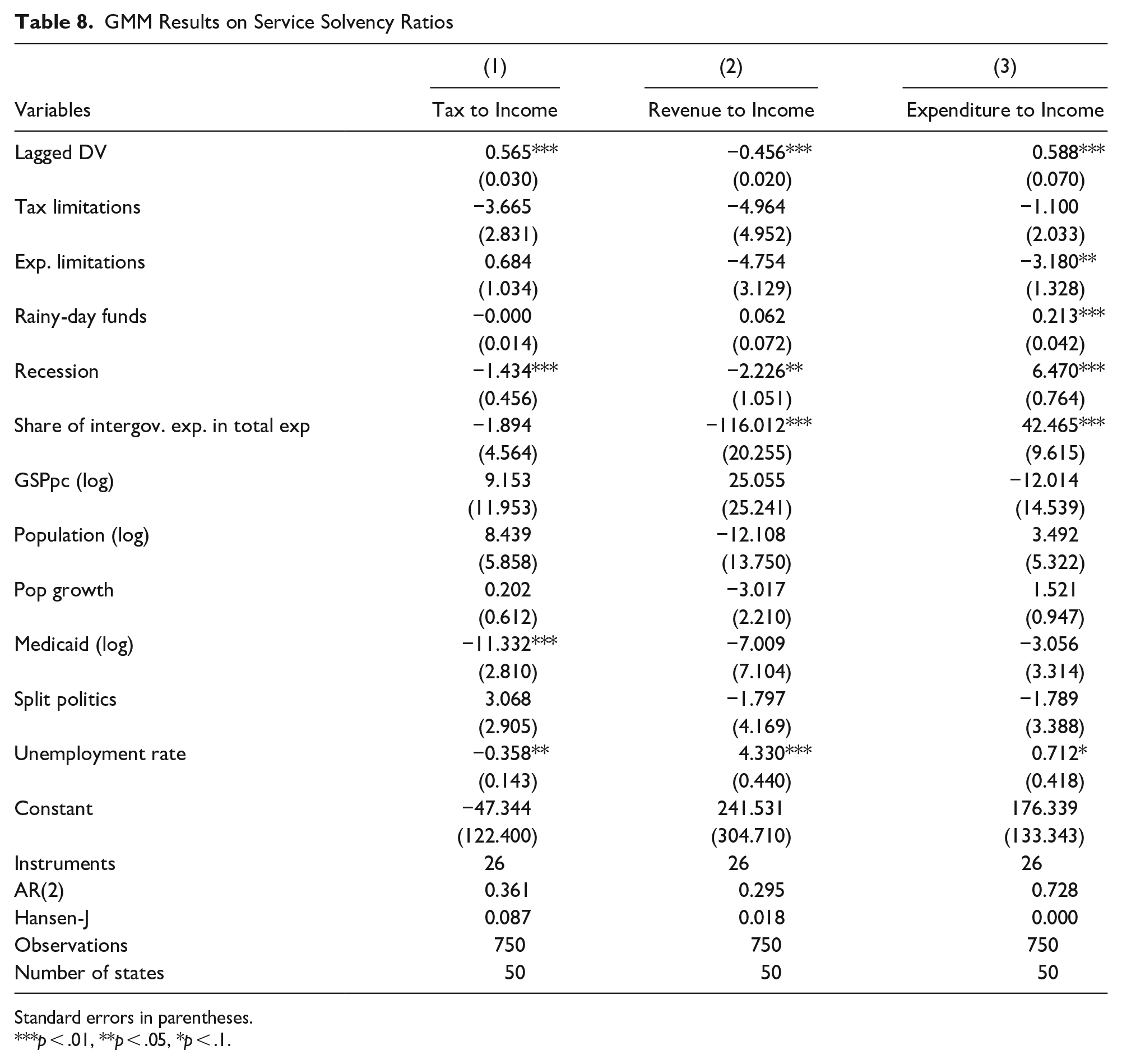
The results of our analysis (reported in Tables 5 through 10) indicate that our first hypothesis (1a) on fiscal illusion is largely true in the sense that the coefficients for tax limitations and/or expenditure limitations are statistically significant in most short-term financial condition ratios. Specifically, expenditure limitations are negative and statistically significant for cash, quick, and current ratios (Table 6). While the sign remains for the composite Cash Solvency index (Table 5), the relationship is not statistically significant. However, stringent expenditure limitations improve the surplus and operating ratios (Table 7), showing a positive and statistically significant relation with the budgetary solvency index (Table 5). Concerning service solvency ratios (Table 8), expenditure limitations are statistically significant only in the expenditure-to-income ratio, showing an adverse relation.

Table 5.

GMM Results on Short-Term Financial Conditions

	(1)	(2)	(3)
Variables	Cash Solvency	Budget Solvency	Service Solvency
Lagged DV	0.946***	−0.203***	0.585***
	(0.175)	(0.075)	(0.036)
Tax limitations	0.693*	−1.577***	0.054
	(0.397)	(0.485)	(0.091)
Exp. limitations	−0.327	0.868*	0.062
	(0.213)	(0.442)	(0.074)
Rainy-day funds	−0.020**	−0.027***	0.006***
	(0.008)	(0.003)	(0.002)
Recession	−0.094	−0.000	0.050
	(0.138)	(0.081)	(0.047)
Share of intergov. exp. in total exp	0.565	3.290**	−0.216
	(1.359)	(1.536)	(0.598)
GSPpc (log)	6.790***	−3.818	−1.102*
	(2.374)	(3.708)	(0.639)
Population (log)	−1.840**	−0.652	0.539*
	(0.877)	(1.156)	(0.286)
Pop growth	0.274	−0.058	0.144
	(0.170)	(0.303)	(0.107)
Medicaid (log)	0.510	0.268	−0.013
	(0.447)	(0.503)	(0.242)
Split politics	−0.547	1.037**	0.284
	(0.583)	(0.427)	(0.221)
Unemployment rate	0.061	−0.085*	−0.011
	(0.037)	(0.047)	(0.017)
Constant	−52.566**	48.823	2.997
	(22.949)	(37.357)	(6.818)
Instruments	26	26	26
AR(2)	0.219	0.208	0.119
Hansen-J	0.524	0.488	0.996
Observations	750	750	750
Number of states	50	50	50

Standard errors in parentheses.

***

p < .01, **p < .05, *p < .1.

Table 6.

GMM Results on Cash Solvency

	(1)	(2)	(3)
Variables	Cash Ratio	Quick Ratio	Current Ratio
Lagged DV	0.645***	0.794***	0.766***
	(0.047)	(0.059)	(0.068)
Tax limitations	0.704	0.956	0.883
	(0.566)	(0.746)	(0.736)
Exp. limitations	−0.655**	−0.725***	−0.670***
	(0.259)	(0.225)	(0.238)
Rainy-day funds	−0.008*	−0.026***	−0.027***
	(0.004)	(0.003)	(0.003)
Recession	−0.122*	−0.161*	−0.196**
	(0.061)	(0.084)	(0.092)
Share of intergov. exp. in total exp	−0.279	0.043	−0.173
	(0.769)	(0.951)	(0.911)
GSPpc (log)	7.361***	10.384***	9.700***
	(2.146)	(2.889)	(2.572)
Population (log)	−0.453	−1.307	−0.543
	(1.001)	(1.494)	(1.558)
Pop growth	0.067	0.256	0.233
	(0.193)	(0.157)	(0.167)
Medicaid (log)	−0.112	−0.161	−0.452
	(0.454)	(0.585)	(0.560)
Split politics	−0.109	−0.170	0.028
	(0.546)	(0.792)	(0.715)
Unemployment rate	0.017	0.037	0.032
	(0.033)	(0.046)	(0.043)
Constant	−69.713***	−89.278***	−89.529***
	(21.611)	(28.716)	(26.889)
Instruments	26	26	26
AR(2)	0.451	0.188	0.275
Hansen-J	0.656	0.450	0.619
Observations	750	750	750
Number of states	50	50	50

Standard errors in parentheses.

***

p < .01, **p < .05, *p < .1.

Table 7.

GMM Results on Budgetary Solvency

	(1)	(2)
Variables	Surplus/deficit PC	Operating Ratio
Lagged DV	−0.388***	0.053
	(0.025)	(0.081)
Tax limitations	−397.408	−0.037
	(425.176)	(0.036)
Exp. limitations	528.546**	0.018
	(250.077)	(0.030)
Rainy-day funds	8.170**	−0.001
	(3.960)	(0.000)
Recession	−186.711***	−0.032***
	(51.791)	(0.006)
Share of intergov. exp. in total exp	−3,002***	−0.456***
	(1,109.277)	(0.136)
GSPpc (log)	−3,170.779	0.070
	(2,275.907)	(0.266)
Population (log)	427.286	0.160*
	(927.508)	(0.089)
Pop growth	−68.053	0.013
	(137.149)	(0.014)
Medicaid (log)	−780.779**	−0.113***
	(317.092)	(0.034)
Split politics	−346.756	0.011
	(327.670)	(0.031)
Unemployment rate	−81.971***	−0.002
	(28.283)	(0.004)
Constant	38,069.543*	−0.612
	(20,906.604)	(2.567)
Instruments	26	26
AR(2)	0.282	0.227
Hansen-J	0.206	0.087
Observations	750	750
Number of states	50	50

Standard errors in parentheses.

***

p < .01, **p < .05, *p < .1.

Table 8.

GMM Results on Service Solvency Ratios

	(1)	(2)	(3)
Variables	Tax to Income	Revenue to Income	Expenditure to Income
Lagged DV	0.565***	−0.456***	0.588***
	(0.030)	(0.020)	(0.070)
Tax limitations	−3.665	−4.964	−1.100
	(2.831)	(4.952)	(2.033)
Exp. limitations	0.684	−4.754	−3.180**
	(1.034)	(3.129)	(1.328)
Rainy-day funds	−0.000	0.062	0.213***
	(0.014)	(0.072)	(0.042)
Recession	−1.434***	−2.226**	6.470***
	(0.456)	(1.051)	(0.764)
Share of intergov. exp. in total exp	−1.894	−116.012***	42.465***
	(4.564)	(20.255)	(9.615)
GSPpc (log)	9.153	25.055	−12.014
	(11.953)	(25.241)	(14.539)
Population (log)	8.439	−12.108	3.492
	(5.858)	(13.750)	(5.322)
Pop growth	0.202	−3.017	1.521
	(0.612)	(2.210)	(0.947)
Medicaid (log)	−11.332***	−7.009	−3.056
	(2.810)	(7.104)	(3.314)
Split politics	3.068	−1.797	−1.789
	(2.905)	(4.169)	(3.388)
Unemployment rate	−0.358**	4.330***	0.712*
	(0.143)	(0.440)	(0.418)
Constant	−47.344	241.531	176.339
	(122.400)	(304.710)	(133.343)
Instruments	26	26	26
AR(2)	0.361	0.295	0.728
Hansen-J	0.087	0.018	0.000
Observations	750	750	750
Number of states	50	50	50

Standard errors in parentheses.

***

p < .01, **p < .05, *p < .1.

Table 9.

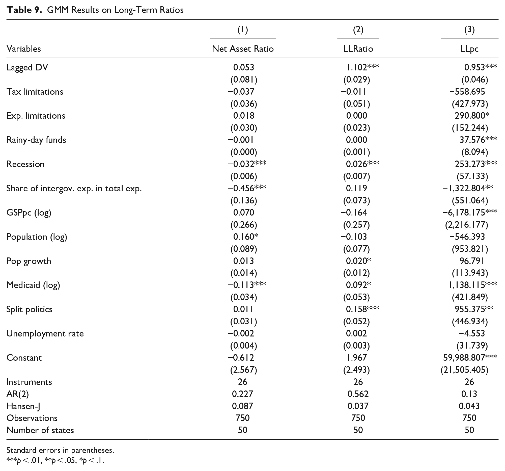
GMM Results on Long-Term Ratios

	(1)	(2)	(3)
Variables	Net Asset Ratio	LLRatio	LLpc
Lagged DV	0.053	1.102***	0.953***
	(0.081)	(0.029)	(0.046)
Tax limitations	−0.037	−0.011	−558.695
	(0.036)	(0.051)	(427.973)
Exp. limitations	0.018	0.000	290.800*
	(0.030)	(0.023)	(152.244)
Rainy-day funds	−0.001	0.000	37.576***
	(0.000)	(0.001)	(8.094)
Recession	−0.032***	0.026***	253.273***
	(0.006)	(0.007)	(57.133)
Share of intergov. exp. in total exp.	−0.456***	0.119	−1,322.804**
	(0.136)	(0.073)	(551.064)
GSPpc (log)	0.070	−0.164	−6,178.175***
	(0.266)	(0.257)	(2,216.177)
Population (log)	0.160*	−0.103	−546.393
	(0.089)	(0.077)	(953.821)
Pop growth	0.013	0.020*	96.791
	(0.014)	(0.012)	(113.943)
Medicaid (log)	−0.113***	0.092*	1,138.115***
	(0.034)	(0.053)	(421.849)
Split politics	0.011	0.158***	955.375**
	(0.031)	(0.052)	(446.934)
Unemployment rate	−0.002	0.002	−4.553
	(0.004)	(0.003)	(31.739)
Constant	−0.612	1.967	59,988.807***
	(2.567)	(2.493)	(21,505.405)
Instruments	26	26	26
AR(2)	0.227	0.562	0.13
Hansen-J	0.087	0.037	0.043
Observations	750	750	750
Number of states	50	50	50

Standard errors in parentheses.

***

p < .01, **p < .05, *p < .1.

Table 10.

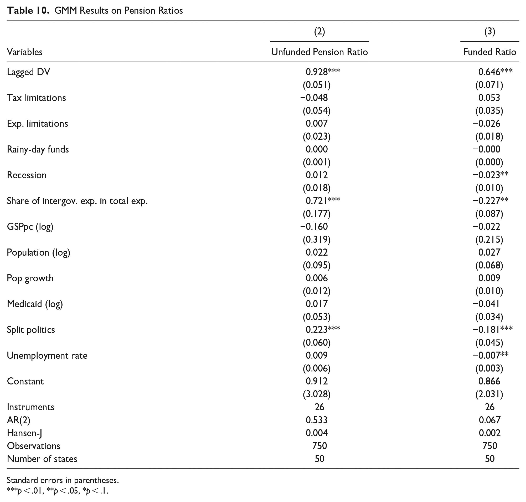
GMM Results on Pension Ratios

	(2)	(3)
Variables	Unfunded Pension Ratio	Funded Ratio
Lagged DV	0.928***	0.646***
	(0.051)	(0.071)
Tax limitations	−0.048	0.053
	(0.054)	(0.035)
Exp. limitations	0.007	−0.026
	(0.023)	(0.018)
Rainy-day funds	0.000	−0.000
	(0.001)	(0.000)
Recession	0.012	−0.023**
	(0.018)	(0.010)
Share of intergov. exp. in total exp.	0.721***	−0.227**
	(0.177)	(0.087)
GSPpc (log)	−0.160	−0.022
	(0.319)	(0.215)
Population (log)	0.022	0.027
	(0.095)	(0.068)
Pop growth	0.006	0.009
	(0.012)	(0.010)
Medicaid (log)	0.017	−0.041
	(0.053)	(0.034)
Split politics	0.223***	−0.181***
	(0.060)	(0.045)
Unemployment rate	0.009	−0.007**
	(0.006)	(0.003)
Constant	0.912	0.866
	(3.028)	(2.031)
Instruments	26	26
AR(2)	0.533	0.067
Hansen-J	0.004	0.002
Observations	750	750
Number of states	50	50

Standard errors in parentheses.

***

p < .01, **p < .05, *p < .1.

While very few studies concern various fiscal condition indicators in relation to TELs and RDFs, multiple studies confirmed that government officials tend to follow the rules associated with different fiscal institutions by resorting to categories that are not directly regulated by the fiscal institution. For instance, Jimenez (2018), in his analysis of local institutional constraints finds that a government circumvents increases in property taxes but does not hesitate to increase fees and other categories not included in the tax limitations. We argue that this could be the case with state administrators as well. We extend our arguments and suggest that state administrators circumvent increases in revenues and direct spending that are directly visible to the voters.

In relation to long-run fiscal health indicators (Tables 9 and 10), expenditure limitations also confirm our hypothesis (1b). Namely, the coefficient is insignificant in two of the long-term debt ratios and both pension ratios. Our finding is not surprising. Maher et al. (2016), for example, in their work on local government, do not find evidence of the impact of TELs on pension funding. The coefficient is positive and statistically significant only in the case of the most transparent long-term ratio, the per capita long-term liabilities. The positive sign for the per capita long-term ratio indicates that more stringent expenditure limits tend to improve the per capita long-term liability.

Unlike expenditure limits, tax limitations have no statistical significance across all individual ratios. They have a positive and statistically significant impact on the cash solvency index and a negative and statistically significant effect on the budget solvency index, but when broken down to the individual ratios, the signs remain for both groups but with no evidence of statistical significance. We also do not find that there is any statistical significance for any of the five ratios that indicate long-term and pension solvencies.

The coefficients for the RDFs are consistently negative and statistically significant in relation to cash and budget solvency indexes and individual ratios, attesting to the tradeoffs between the required RDFs and short-term fiscal health. While RDFs are used to alleviate fiscal shocks, at other times, states tend to increase RDFs for highly obvious reasons, namely, to improve credit rating (Grizzle, 2010). However, the estimates for RDFs are positive and significant for the expenditure-over-income ratios and positive and marginally significant for the overall service solvency index, indicating that RDFs positively influence service delivery.

Similar to the findings on TELs, RDFs do not have a statistically significant impact on all long-term (Table 9) and pension ratios (Table 10), except in the case of the most visible per capita long-term liability ratio. This relation has a positive sign, indicating that RDFs tend to increase per capita long-term liability.

As for control variables, there are several interesting observations. First, regarding short-term solvencies, divided government turned out to be significant only for budgetary solvency, indicating a shared governance is beneficial for budgetary solvency. However, split governance tends to increase both the long-term liability ratio and the per capita long-term liability. It also reduces the unfunded pension ratio, while improving the funded pension ratio. Some of the economic and demographic factors are significant, but they had different impacts on different short-term financial conditions. For instance, population size is negatively related to cash solvency but positively related to budgetary solvency. In contrast, per capita gross state product positively affects both cash solvency and service solvency. Regarding the control variables in the regressions on individual financial ratios, we found that per capita gross state product is consistently positively associated with cash solvency. Expectedly, higher per capita GSP reduces per capita long-term liabilities. Recession and the share of intergovernmental expenditure are consistently significant across various budgetary and service solvency ratios. So are the coefficient estimates for Medicaid beneficiaries and the unemployment rate. In the regression on individual long-term financial condition ratios, the control variables that stand out are recession, share of intergovernmental expenditure, Medicaid beneficiaries, and split government which are statistically significant.

Conclusion

Using the panel data from the states’ annual comprehensive financial reports for the period 2003 to 2018, we analyzed how the disaggregated TELs and RDFs affect state fiscal condition by using the GMM. After controlling for a number of political and socioeconomic factors, our analysis suggests that TELs affected the state government’s short-term but not long-term financial conditions, except when the information regarding long-term debt is publicly available, such as in the case of per capita long-term debt. The fiscal illusion lens provides us with a theoretical framework to understand this interesting pattern. Conversely, our empirical results provide evidence for such a hypothesis regarding the preference of state government in debt financing and the preference to shift financial obligations to the future. In addition, we found a similar effect of the RDFs on the state government’s financial condition.

Our study provides a more nuanced understanding of the implications of TELs and RDFs on short-term fiscal conditions. That is, we provide empirical evidence that there are tradeoffs when it comes to the level of stringency in limiting government taxes and expenditures. While the level of RDFs could improve all short-term solvency indicators, it seems that they compete with both cash and budget ratios.

The findings from this study have important implications for a better understanding of the state-level strategies and the long-term and pension funding behaviors. While the fiscal illusion theory has been studied in the government finance setting since its inception, scholars have been mostly concerned with the tax structure concerning distorted citizen perceptions due to imperfect information flow from the government to the citizen. The empirical evidence in our study suggests that neither TELs nor RDFs are impacting pension and long-term debt, confirming the underlying fiscal illusion assumption that governments tend to manipulate spending and revenue categories that are less visible to the regular citizen. Moreover, the findings from our study provide convincing evidence that institutional constraints such as tax limits and expenditure limits matter for short-term and highly visible categories such as cash and budget solvencies. Our analysis allows a state-level comparison over an extended period, thus providing insights into the implications of these major fiscal institutions in the long run.

There are also practical implications for policymakers and administrators. For state policymakers, it is important to be aware of the practical implications of passing new fiscal policies that are intended to address some priority goals, as there may be some unintended consequences for short-run and long-run financial conditions. For administrators in state finances, this study explains how different fiscal policies influence various aspects of solvency for fiscal planning and management. The findings concerning the relations of financial condition will help state budget makers and financial managers understand the potential impact of fiscal policies, i.e. tax and expenditure limits, RDFs, as well as politics and budgetary and demographic factors on financial condition. However, our research comes with limitations. First, future research may extend the research by including data from more recent years, especially during the COVID-19 pandemic. Second, the analysis can be more thorough with more data on state fiscal policies. For instance, if data on deposit and withdrawal rules of RDFs are available, future research can examine the compound effect of RDFs on a state’s financial condition.

Footnotes

Declaration of Conflicting Interest

The author(s) declared no potential conflicts of interest with respect to the research, authorship, and/or publication of this article.

Funding

The author(s) received no financial support for the research, authorship, and/or publication of this article.

Notes

References

Amiel

Deller

Stallmann

(May 2009). The construction of a tax and expenditure limitation index for the U.S. Agricultural & Applied Economics. Staff Paper No. 536.

Amiel

Deller

Stallmann

Maher

(2014). Does the restrictiveness of state tax and expenditure limitations affect state revenues and expenditures? International Journal of Public Administration, 37, 237–248. https://doi.org/10.1080/01900692.2013.812113

Anderson

T. W.

Hsiao

(1982). Formulation and estimation of dynamic models of panel data. Journal of Econometrics, 18(1), 47–82. https://doi.org/10.1016/0304-4076(82)90095-1

Arellano

Bond

(1991). Some tests of specification for panel data: Monte Carlo evidence and an application to employment equations. Review of Economic Studies, 58(2), 277–297. https://doi.org/10.2307/2297968

Arellano

Bover

(1995). Another look at the instrumental variables estimation of error components models. Journal of Econometrics, 68(1), 29–52. https://doi.org/10.1016/0304-4076(94)01642-D

Arnett

(2014, January 2014). State Fiscal Condition Ranking the 50 States. George Mason University Mercatus Center, Working Paper, No. 14-02. https://dx.doi.org/10.2139/ssrn.3211617

Bae

Moon

S.-G.

Jung

(2012). Economic effects of state-level tax and expenditure limitations. Public Administration Review, 72(5), 649–658. https://doi.org/10.1111/j.1540-6210.2012.02571.x

Blundell

Bond

(1998). Initial conditions and moment restrictions in dynamic panel data models. Journal of Econometrics, 87(1), 115–143. https://doi.org/10.1016/S0304-4076(98)00009-8

Boccia

(2022). Fiscal Illusion and Deficit Spending. Retrieved from https://policycommons.net/artifacts/3344873/fiscal-illusion-and-deficit-spending/4143753/

10.

Brown

K. W.

(1989). Ten-point test of financial condition: Toward and easy-to-use assessment tool for small cities. Government Finance Review, 9(6): 21–26.

11.

Buchanan

J. M

Wagner

R. E.

(1977). Democracy in deficit: The political legacy of Lord Keynes. Academic Press.

12.

Cabaleiro

Buch

Vaamonde

(2013). Developing a method to assessing the municipal financial health. The American Review of Public Administration, 43(6), 729–751. https://doi.org/10.1177/0275074012451523

13.

Clark

Y. B.

(2015). Evaluating the validity and reliability of the financial condition index for local governments. Public Budgeting & Finance, 35(2), 66–88. https://doi.org/10.1111/pbaf.12063

14.

Dell’Anno

Dollery

E. B.

(2014). Comparative fiscal illusion: A fiscal illusion index for the European Union. Empirical Economics, 46: 937–960.

15.

Ermasova

Kulik

J.M.

(2018) The Effects of Tax and Expenditure Limitation (TEL) Stringency on the Level of State Expenditures in the United States. Review of Public Administration Management, 6, 1. https://doi.org/10.4172/2315-7844.1000236

16.

Gorina

Maher

Joffe

(2017). Local fiscal distress: Measurement and prediction. Public Budgeting and Finance, 38(1), 72–94. https://doi.org/10.1111/pbaf.12165

17.

Government Accounting Standard Board. (1999). Summary of Statement No. 34. https://gasb.org/page/PageContent?pageId=/standards-guidance/pronouncements/summary–statement-no-34.html&isStaticPage=true

18.

Grizzle

(2010). The impact of budget stabilization funds on state general obligation bond ratings. Public Budgeting & Finance, 30(2), 95–111. https://doi.org/10.1111/j.1540–5850.2010.00958.x

19.

Groves

M.S.

Valente

G. M.

(1986). Evaluating financial conditions: A handbook for local government ICMA.

20.

Hoang

Maher

S. C.

(2022). Fiscal condition, institutional constraints, and public pension contribution: Are pension contribution shortfalls fiscal illusion? Public Budgeting & Finance, 42(4): 93–124. https://doi.org/10.1111/pbaf.12328

21.

Hou

(2003). What stabilizes state general fund expenditures in downturn years—budget stabilization fund or general fund unreserved undesignated balance? Public Budgeting & Finance, 23(3), 64–91. https://doi.org/10.1111/1540-5850.2303004

22.

Hou

(2005). Fiscal reserves and state own-source expenditure in downturn years. Public Finance Review, 33(1): 117–144. https://doi.org/10.1177/1091142104271139

23.

Hou

Brewer

A. G.

(2010). Substitution and Supplementation between Co-Functional Policy Instruments: Evidence from State Budget Stabilization Practices. Public Administration Review, 70(6), 914–24. https://doi.org/10.1111/j.1540-6210.2010.02223.x

24.

Jimenez

S. B.

(2018). Fiscal institutional externalities: The negative effects of local tax expenditure limits on municipal budgetary solvency. Public Budgeting and Finance, 38, 3–31. https://doi.org/10.1111/pbaf.12194

25.

Kallen

(2017, September 2017). State tax expenditure limitation and supermajority requirement: New and updated data. American Enterprise Institute Working paper, 2017–19.

26.

Kioko

N. S.

(2013) Reporting on the financial condition of the states: 2002-2010. Journal of Public Budgeting, Accounting & Financial Management, 25(1), 165–198.

27.

Kloha

Weissert

S. K.

Kleine

(2005) Developing and Testing a composite model to predict local fiscal distress. Public Administration Review, 65(3), 313–323. https://doi.org/10.1111/j.1540-6210.2005.00456.x

28.

Lee

(2014). The effect of supermajority vote requirements for tax increase in California: A synthetic control method approach. State Politics & Policy Quarterly, 14(4), 414–436. https://doi.org/10.1177/1532440014556050

29.

Lee

(2018). Do States circumvent constitutional supermajority voting requirements to raise taxes? State Politics & Policy Quarterly, 18(4), 417–440. https://doi.org/10.1177/1532440018796811.

30.

Maher

(2013). Financial condition: An essential element of management during periods of fiscal stress. The Journal of Government Financial Management, 62(1), 20–25. https://doi.org/10.1108/JPBAFM-23–03-2011-B006

31.

Maher

S. C.

Deller

C. S.

(2010, February 25–27). Measuring the impacts of TELs on municipal financial conditions. In Paper prepared for States as Facilitators or Obstructionists of Local Governments Conference.

32.

Maher

S. C.

Deller

C. S.

(2011). Measuring municipal fiscal condition: Do objective measures of fiscal health relate to subjective measures. Journal of Public Budgeting, Accounting & Financial Management, 25(2), 165–198. https://doi.org/10.1108/JPBAFM-23-03-2011-B006

33.

Maher

S.C.

Park

Harrold

(2016). The effects of tax and expenditure limits on municipal pension and OPEB funding during the Great Recession. Public Finance and Management, 16(2), 121–146. https://doi.org/10.1177/152397211601600203

34.

Maher

S. C.

Nollenberger

(2009). Revisiting Kenneth Brown’s 10-point test. Government Finance Review, 25(5), 61–66.

35.

Maher

S.C.

Park

McDonald

B.D.

Deller

S.C.

(2023). Understanding municipal fiscal health: A model for local governments in the USA. Routledge.

36.

Maher

S. C.

Stallmann

I. J.

Deller

C. S.

Park

(2017). The effects of tax and expenditure limits on state fiscal reserves. Public Policy and Administration, 32(2): 130–151. https://doi.org/10.1177/0952076716660607

37.

Miller

J.M.

Lin

(2005). What can the “price of government” predict? Proceedings of the Annual Conference of the National Tax Association, 98: 507–513.

38.

Mullins

R. D.

Joyce

G. P.

(1996). Tax and expenditure limitations and state and local fiscal structure: An empirical assessment. Public Budgeting & Finance, 16, 75–101. https://doi.org/10.1111/1540-5850.01061

39.

Mullins

R.D.

Wallin

B.A.

(2004). Tax and expenditure limitations. Public Budgeting & Finance, 24(4), 2–15.

40.

NASBO (2023). State Expenditure Report. Fiscal Years 2021-2023. Retrieved from https://higherlogicdownload.s3.amazonaws.com/NASBO/9d2d2db1-c943-4f1b-b750-0fca152d64c2/UploadedImages/SER%20Archive/2023_State_Expenditure_Report-S.pdf

41.

Navarro-Galera

Rodríguez-Bolívar

P. M.

Alcaide-Muñoz

López-Subires

D. M.

(2016). Measuring the financial sustainability and its influential factors in local governments. Applied Economics, 48(41), 3961–3975. https://doi.org/10.1080/00036846.2016.1148260

42.

Niskanen

Jr. (1971). Bureaucracy and representative government. Aldine.

43.

Niskanen

Jr. (1994). Bureaucracy and public economics. Edward Elgar.

44.

Nollenberger

Groves

S. M.

Valente

M. G.

(2003). Evaluating financial condition: A handbook for local government. International City/County Managers Association.

45.

Norcross

Gonzalez

(2018). Ranking the states by fiscal condition. Mercatus Center, George Mason University. Retrieved October 2020, from www.mercatus.org/statefiscalrankings

46.

Poterba

J. M

. (1994). State responses to fiscal crises: The effects of budgetary institutions and politics. Journal of Political Economy, 102(41):, 799–821.

47.

Rivenbark

C. W.

Roenigk

J. D.

Allison

S. G.

(2010). Conceptualizing financial condition in local government. Journal of Public Budgeting, Accounting & Financial Management, 22(1), 149–177.

48.

Roodman

(2009a). A note on the theme of too many instruments. Oxford Bulletin of Economics and Statistics, 71(1), 135–158. https://doi.org/10.1111/j.1468-0084.2008.00542.x

49.

Roodman

(2009b). How to do xtabond2: An introduction to‘difference’and‘system’GMM in Stata. The Stata Journal, 9(1): 86–136. https://doi.org/10.1177/1536867X0900900106

50.

Ryu

Cho

Kim

(2020). Does the stringency of state tax and expenditure limitations discourage political manipulation in fiscal reserves? Public Administration Review, 81(3), 375–388. https://doi.org/10.111/puar.13306

51.

Seljan

E.C.

(2014). The limits of tax and expenditure limits: TEL implementation as a principal-agent problem. Public Choice, 159(3–4), 485–501

52.

Shi

(2020). Using fuzzy logic to evaluate and compare state financial condition during and after the Great Recession of 2008: Fuzzy rule-based systems. Public Administration Quarterly, 44(3), 394–432. https://doi.org/10.37808/paq.44.3.3

53.

Singla

Stone

B. S.

(2018). Fiscal decentralization and financial condition: The effects of revenue and expenditure decentralization on state financial health. State and Local Government Review, 50(2), 119–131. https://doi.org/10.1177/0160323X18794014

54.

Skidmore

(1999) Tax and expenditure limitations and the fiscal relationships between state and local governments. Public Choice, 99(1–2), 77–102.

55.

Sohl

Peddle

T. M.

Thurmaier

Wood

H. C.

Kuhn

(2009). Measuring the financial position of municipalities: Numbers do not speak for themselves. Public Budgeting & Finance, 29, 74–96. https://doi.org/10.1111/j.1540-5850.2009.00937.x

56.

Stallmann

I. J.

Maher

S. C.

Deller

C. S.

Park

(2017). Surveying the effects of limitations on taxes and expenditures: What do/Don’t we know? Journal of Public and Nonprofit Affairs, 3(2), 197–222.

57.

Stone

B. S.

(2015). The effect of fiscal decentralization on the financial condition of municipal government. International Journal of Public Administration, 38, 453–460. https://doi.org/10.1080/01900692.2014.949740

58.

Stone

B. S.

Singla

Comeaux

Kirschner

(2015). A Comparison of fiscal indicators: The Case of Detroit. Public Budgeting and Finance, 35(4), 90–111. https://doi.org/10.1111/pbaf.12079

59.

Tax Policy Center. (2020). Briefing book: The state of state (and local) tax policy. https://www.taxpolicycenter.org/briefing-book/what-are-state-rainy-day-funds-and-how-do-they-work

60.

Tempelman

H. J.

(2007). James M. Buchanan on Public-Debt Finance. The Independent Review, 11(3), 435–449

61.

Turley

Robbins

McNena

(2015). A framework to measure the financial performance of local governments, Local Government Studies, 41(3): 401–420. https://doi.org/10.1080/03003930.2014.991865

62.

Wagner

A. G.

(2003). Are state budget stabilization funds only the illusion of savings? Evidence from stationary panel data. The Quarterly Review of Economics and Finance, 43: 213–238. https://doi.org/10.1016/S1062-9769(01)00132-6

63.

Wang

Dennis

Y, S

. (2007). Measuring Financial Condition: A Study of U.S. States. Public Budgeting & Finance, 27(2), 1–21. https://doi.org/10.1111/j.1540-5850.2007.00872.x

64.

Wei

Denison

V. D.

(2019). State rainy day funds and government general fund expenditures: Revisiting the Stabilization Effect. Public Finance Review, 47(3), 465–492. https://doi.org/10.1177/1091142118819991

65.

Yan

Carr

A. D.

(2019). Impact of revenue diversification and revenue elasticity on state fiscal health. Public Finance and Management, 19(2), 151–174. https://doi.org/10.1177/152397211901900203

State Fiscal Policies and Financial Condition: A Panel Data Analysis of U.S. State Tax and Expenditure Limits and Rainy-Day Funds

Abstract

Keywords

Literature Review

Tax and Expenditure Limits

Rainy-Day Funds

Evaluating Financial Condition

Data and Methodology

Dependent Variables

Measuring Policy and Control Variables

Empirical Model

Results and Discussions

Conclusion

Footnotes

Declaration of Conflicting Interest

Funding

Notes

References