
Abstract
Despite the extensive theoretical connections between defense budget growth and inflation, empirical findings based on traditional time-domain methods have been inconclusive. This study reexamines the issue from a time–frequency perspective. Applying continuous wavelet analysis to the U.S. and Britain, it shows empirical evidence in support of positive bilateral effects in both cases. In the bivariate context, U.S. defense budget growth promoted inflation at 2- to 4-year cycles in the 1840s and at 8- to 24-year cycles between 1825 and 1940. Conversely, inflation accelerated defense spending growth at 5- to 7-year cycles in the 1830s and at 25- to 64-year cycles between 1825 and 1940. Similarly, British defense budget growth spurred inflation at 8- to 48-year cycles between 1890 and 1940 and at 50- to 65-year cycles between 1790 and 1860. Inflation fueled the growth of defense spending at 7- to 20-year cycles between 1840 and 1870, in the 1940s, and in the 1980s. Preliminary results from multivariate analyses are also supportive, though there is a need for further research that is contingent on advancements in the wavelet method in the direction of simulation-based significance tests.
Introduction
The socioeconomic consequences of expansionary defense spending have long been a subject of academic interest. For macroeconomists and central bankers, this field is critical for evaluating how fiscal policy instruments enhance the overall performance of the economy. For political economists, it offers a classic example of how government decisions based on political calculations can distort the self-governance of the market. National security strategists and peace scientists can use new insights in this area to better assess the feasibility of national security policies. Given the significance of the question, it is not surprising to see ever-growing research interest in topics such as the guns–butter trade-off in government budget formation and its implications for socioeconomic development.
As part of the broader inquiry into the socioeconomic consequences of expansionary defense spending, this study empirically tackles the nexus between defense budget growth and inflation. The current research is motivated by a puzzle that becomes immediately apparent upon review of the present literature. On one hand, writings by macroeconomists, political economists, and peace scientists have provided multiple mechanisms by which interplays between defense budget growth and inflation can be theoretically established. On the other hand, empirical findings on the issue have been highly ambiguous and inconclusive. This research argues that the inconsistency between the theoretical expectation and the empirical result is a reflection of the methodological challenges posed by the complicated relationship between defense budget growth and inflation. Specifically, the challenges can be summarized in four aspects. They are cross-national heterogeneity, demand for long time-series data, the nonlinear relationship between defense budget growth and inflation, and the need to separate the variance in the frequency domain from that in the time domain. With due attention paid to the four methodological challenges, this study reexamines the relationship from a time–frequency perspective. By applying continuous wavelet analysis to the U.S. from 1793 to 2019 and Britain from 1751 to 2019, this study shows empirical evidence in support of positive bilateral effects between defense budget growth and inflation in both the cases.
The rest of this study is organized as follows. Part 2 reviews the theoretical and empirical writings on the nexus between defense budget growth and inflation. Part 3 introduces the data and method involved. Part 4 operates bivariate analysis and reports the results. Part 5 provides a preliminary analysis in a multivariate context. Part 6 concludes by summarizing the findings of this study, highlighting their implications, and pointing out valuable research directions for the future.
The Nexus Between Defense Budget Growth and Inflation
The positive effect of expansionary defense spending on inflation can be theoretically established through the following four mechanisms. First, an increase in defense spending might increase inflation from the demand side. According to both the classical and Keynesian models, inflation occurs when the aggregate demand exceeds the aggregate supply (Abel et al., 2014). Because defense spending takes up a considerable portion of the overall government budget, and that budget is in turn an integral part of the aggregate demand, unless expansionary defense spending is offset by higher taxes and/or lower spending in other areas, it can give rise to inflation through the well-known mechanism of demand-pull (Hartman, 1973; Schultze, 1981). Regarding the question of why the government would increase defense spending even during peacetime, the answers can be divided into a Keynesian camp and a political economy camp. The Keynesian version sees defense spending as a crucial fiscal instrument for addressing unemployment and recession (Alptekin and Levine, 2012; Atesoglu, 2002; Nincic and Cusack, 1979). The political economy version, by contrast, emphasizes the role of ambitious politicians, budget-maximizing bureaucrats, defense industry lobbyists, or some combination of the three in pushing for greater defense spending (Calleo, 1981; Kaufman, 1972; Niskanen, 1968, 1996). It is important to note, however, that the division between the two camps of reasoning is not mutually exclusive, because government decisions to reduce unemployment and boost the economy might ultimately be motivated by political concerns such as an incumbent official’s desire to win reelection.
Second, an increase in defense spending can promote inflation from the supply side. The defense industry has long been characterized by oligopoly. The limited number of suppliers means there is likely to be a bottleneck in production when there is a sudden increase in demand (Capra, 1981; Fordham, 2003). At the same time, the lack of competition in the defense market allows suppliers to maintain a cost-maximizing fashion of production while still enjoying high profit margins. Meanwhile, political economists are pessimistic about the government’s desire and ability to correct the prevailing high costs and low productivity in the industry, given the existence of information asymmetry, rent-seeking behavior of government officials, and the pressure politics of defense-related interest groups. All of these naturally contribute, in a cost–push fashion, to sectoral inflation that will transmit itself to other parts of the economy (Vitaliano, 1984).
Third, defense budget growth can increase inflation through monetary policy. Monetarist scholars argue that inflation is ultimately a monetary phenomenon that occurs when the supply of money grows more rapidly than the real output of an economy (Friedman and Schwartz, 1971). Since the defense budget is part of fiscal policy, it does not have an immediate impact on inflation, according to monetarism. An indirect connection, however, can be established if an increase in defense spending gives rise to a fiscal deficit, and the monetary authority decides to finance the deficit by creating and circulating more currency (Friedman, 1989). In line with this reasoning, many political economists have pointed out that governments have a strong incentive to cover defense-related costs through inflation rather than additional taxes or spending cuts in other areas (Hamilton, 1977; Heo and Bohte, 2011; Rockoff, 2015). It is important to note that some macroeconomists question the significance of the monetary authority’s decision to finance the deficit. Instead, they argue that a fiscal deficit ultimately gives rise to inflation if fiscal authority dominates the monetary authority (Ljungqvist and Sargent, 2012; Sargent, 2013; Sargent and Wallace, 1981).
Finally, the impact of a growing defense budget on the balance of payments provides another channel through which expansionary defense spending can positively affect inflation (Starr et al., 1984). When the defense budget is spent heavily abroad for purposes such as overseas operations or importing military equipment, it may amount to a substantial balance-of-payments deficit. If the government generates money to finance the deficit, it can trigger a depreciation of the local currency’s exchange rate. The resulting increase in the price of imported goods combined with the decrease in price of the country’s exports then promotes domestic inflation via the cost–push and demand–pull mechanisms, respectively. Scholars have noted, however, that the situation is more likely to occur in small- and medium-sized economies. Great powers whose currency is widely used in international business transactions are significantly less likely to face this problem (Krugman and Wells, 2015).
The effect of inflation on defense budget growth can be either positive or negative in theory (Capra, 1981; Kaufman, 1972; Starr et al., 1984). On one hand, inflation increases the cost of defense-related products and services by reducing the purchasing power of the local currency. An increase in defense spending is then required to counterbalance that lower purchasing power and maintain the real output of defense-related items. In practice, supporters of expansionary defense spending often use inflation as a reason to advance their argument, and fiscal decision-makers consider inflation a critical factor in their budget planning. In this scenario, inflation increases the defense budget.
On the other hand, inflation can also lead government officials to consider cutting the defense budget for at least two reasons. First, the government might use a defense budget cut as a fiscal instrument to contain inflation. Second, the loss in the purchasing power of the local currency may intensify the budgetary competition between guns and butter. When incumbent politicians are less concerned with security, they are more likely to make a trade-off at the expense of defense spending.
From the analysis above, it is not hard to appreciate the potentially bilateral effects. On one hand, defense budget growth can promote inflation through the mechanisms of demand–pull, cost–push, monetary policy, and the balance of payments in an open economy. On the other hand, higher inflation can influence the growth of defense spending either positively or negatively, depending on the policy priorities of the government in office. If the government prefers to maintain the level of defense output, the effect is positive. When the government prefers to control inflation, and external security is low on the policy agenda, the impact should be negative. Thus, some scholars in the field claim that the relationship between defense budget growth and inflation is actually bilateral (Starr et al., 1984; Xu et al., 2020).
Despite the popular arguments on the theoretical connectivity between defense budget growth and inflation, empirical findings on the topic have been highly ambiguous and inconclusive. Empirical inquiry into the question began with developed economies. Using data from the U.S., Vitaliano (1984) rejects the hypothesis that a rapid growth in defense spending contributes to inflation. Follow-up research by Nourzad (1987) comes to a different conclusion, while that by Sahu et al. (1995) reconfirms Vitaliano’s position that an increase in defense spending is not inflationary. Using data between 1956 and 1979, Starr and colleagues (Starr et al., 1984) report that defense budget growth and inflation are mutually reinforcing in France and the Federal Republic of Germany, but there is no significant relationship between them in the United States and the United Kingdom. Although early research on developing countries suggests that greater defense spending is likely to increase inflation (Chan, 1977; Chowdhury, 1991; Deger and Smith, 1983), other studies have found that the newly industrialized economies of Asia could be notable exceptions (Chan and Davis, 1991; Lin et al., 2016). More recently, the rise of China as a global economic and military power has led scholars to study the defense–inflation nexus in the Middle Kingdom. Findings are again confusing. For instance, Lin et al. (2016) report that expansionary defense spending in China generates domestic inflation in the long run. However, Xu et al. (2020) reject this idea in a study showing that inflation in China slows the growth of defense spending at least in peacetime.
Besides the research on the nexus between defense budget growth and inflation, a related set of literature explores the relationship between major wars involving great powers and price inflation. Although political historians of the literature collected anecdotal evidence from Europe and the U.S. indicating that major wars in the modern age tend to be increasingly inflationary (Hamilton, 1977; Rockoff, 2015), findings from empirical studies are far from conclusive. For instance, Goldstein (1988) claims that in long-run cycles, major wars have consistently had a positive effect on inflation during the post-Napoleonic period. However, the validity of this position has been challenged, to various degrees and on different methodological grounds, by other researchers (Aguiar-Conraria et al., 2012; Beck, 1991; Thompson and Zuk, 1982).
This research argues that the ambiguous empirical results in the present literature are a reflection of the methodological challenges posed by the complicated relationship between defense budget growth and inflation. First of all, the heterogeneity across countries makes it almost impossible to make generalized statements regarding the issue. Thus, scholars in the field generally agree that it is more appropriate to tackle the question on a country-by-country basis. Second, the mixed results might be due to the various time horizons adopted by different researchers. This inconvenient fact is worrisome. Suppose a theory predicts that the effect of defense spending growth on inflation will emerge in the long run, but empirical studies cover only a short span to test the theory. The lack of a significant effect between the relevant variables then does not provide any hard evidence for assessing the theoretical prediction. Unfortunately, the lack of long time-series data is the norm for most of the existing empirical research on the defense–inflation nexus. Due to this concern, it is obviously preferable to have a data set that covers a reasonably extended period of time. Third, the relationship between defense budget growth and inflation might be context specific and hence have nonlinear dynamics. Even for the same country, the connections between defense budget growth and inflation might emerge only during certain periods of history. This is because the occurrence of structural breaks can change the significance, magnitude, and direction of the defense–inflation nexus. Finally, the ambiguous results in the present literature might be the outcome of a mismatch between the theoretical question at stake and the methodological tools in use. Theoretically, the relationship between defense budget growth and inflation might vary across different economic cycles. Thus, it is necessary to separate the variance in the frequency domain from that in the time domain. However, traditional time-domain methods, the powerhouse of the existing literature, are not conducive to this. Therefore, new research methods are needed. In conclusion, researchers must pay due attention to the four methodological challenges mentioned above for a better understanding of the defense–inflation nexus. Following this logic, the next section introduces the data and method of this research with an eye to these challenges.
Data and Method
This study reexamines the relationship between defense spending growth and inflation in the United States and Britain. There are four reasons for this choice of countries. First, scholars in the field generally agree that a case-by-case approach is more fruitful, given the heterogeneity across countries. Second, as the two consecutive global hegemons in modern history, Britain and the U.S. constitute their own category. Findings regarding the hegemons are of both intellectual and practical interest. Third, the theoretical inquiry into the question starts with the U.S., and Britain suggests a likely bilateral relationship. However, it is intellectually puzzling as to why extensive empirical investigations of these countries have failed to provide conclusive evidence in support of the claim. Finally, recent data collection efforts have increased the availability of long time-series data from the two countries.
Defense budget data for the U.S. and Britain come from Chantrill (2019) and Chantrill, (2020), respectively. Following Starr et al. (1984), the growth rate is calculated by using the current value of the two countries’ respective currencies. The data on CPI-based inflation in the U.S. and Britain are collected from Webster (2020a, 2020b), respectively. Combining the data, we end up with observations of the U.S. from 1793 to 2019 and observations of Britain from 1751 to 2019. The time coverage is decided entirely by the availability of data.
The data are analyzed by continuous wavelet transformation (CWT), a time–frequency approach that can separate variance in the frequency domain from that in the time domain. The method was first developed by Morlet et al. (1982a, 1982b); in an effort to give time-localized estimates of frequency content on the basis of research done by Gabor (1946). Although the research originated in the study of geophysics, it soon gained recognition from mathematicians who have continuously contributed to the development of the literature (Woodward et al., 2017). Early statistical theories of the method are nicely summarized in Heil and Walnut (2006), and applications can be found in Vidakovic (1999) and Antoniadis (2007). Today, the method has won popularity in many scientific disciplines, including physics, engineering, environmental science, and life science (Crowley, 2007). Among social scientists, economists pioneered the use of wavelet-based methods in the 1990s (Ramsey et al., 1995; Ramsey and Lampart, 1998). Since then, the application of the technique has grown steadily in analyzing financial and macroeconomic series where periodicity, nonlinearity, and nonstationarity are typically involved (Gallegati and Semmler, 2014; In and Kim, 2013). Take the study of inflation, for instance. The Google Scholar search engine returns more than 10,000 results that applied wavelet-based analysis to inflation, indicating the appropriateness of our choice of model.
The following instruction of CWT works only as a review of the critical concepts and measures included in this study. More comprehensive reviews of the method for social scientists can be found in Aguiar-Conraria et al. (2013). To operate wavelet analysis, we need first to identify a mother wavelet
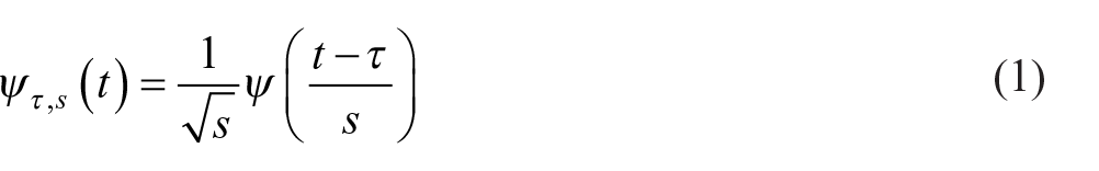
For a single time series
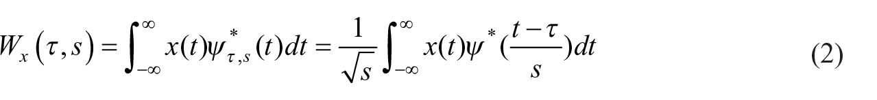
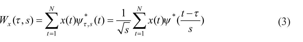
where * denotes the conjugate form. In practice, the time series
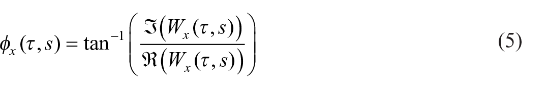
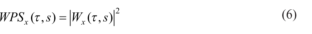
When the mother wavelet is a complex one, the CWT of a time series

where
where
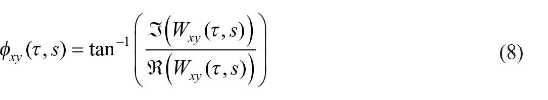
For two time series

The direction of effects between the two series can then be inferred from the cross-wavelet phase angle
If
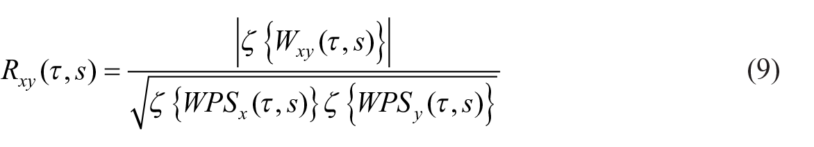
where
This research adopts the Morlet wavelet for CWT. The wavelet is defined as
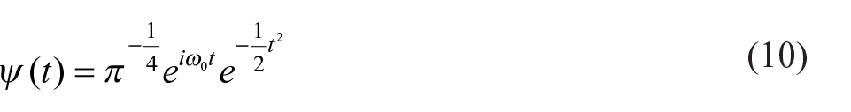
where
Results
The Case of the United States
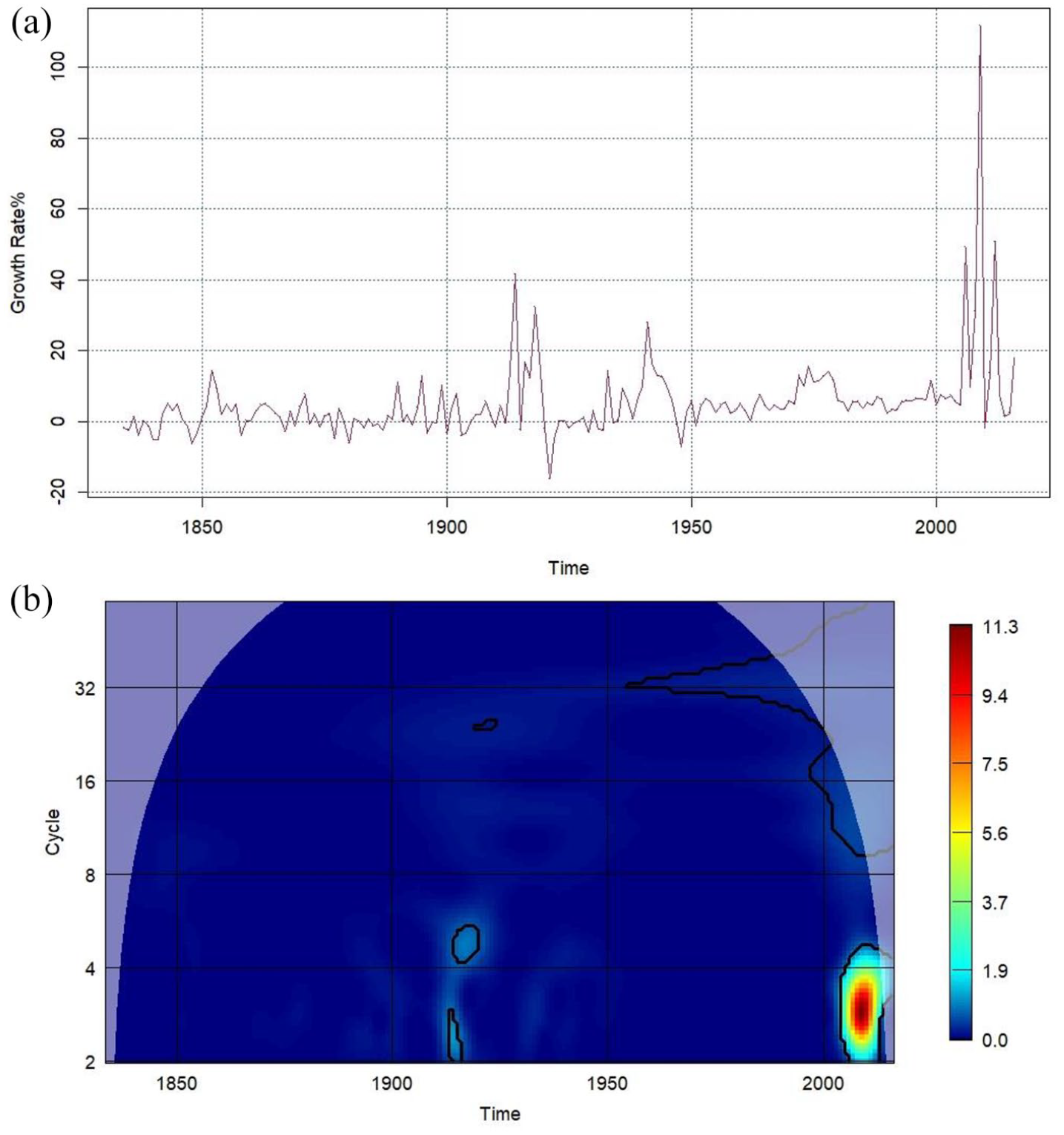
Figure 1(a) and (b) shows U.S. defense budget growth and its power spectrum, respectively. The most noticeable vibrations in the defense budget are associated with war. Throughout the period, the outbreak of the American Civil War and the U.S. entry into World War I are the two most significant events, both of them increasing the defense budget by more than 1100%. The spikes are so striking that they dwarf the defense budget increases that accompanied the War of 1812 and the official U.S. entry into World War II after the attack on Pearl Harbor. The depiction of the power spectrum maps defense budget growth onto a time–frequency plane. For the convenience of interpretation, cycles rather than frequencies are reported throughout the article. The thermal scheme highlights the variance. The contour lines indicate the 5% level of significance. Following Torrence and Compo (1998), the level of significance is assessed against surrogate data generated by 5000-time Monte Carlo simulations of the red-noise process. Results based on other data-generating processes are available upon request, and they do not qualitatively change the conclusions drawn in this article. The translucent area is the cone of influence (COI) that is introduced to deal with the edge effect of CWT. The results shown in the COI are artifacts and should thus be ignored. According to Figure 1(b), the variance of U.S. defense spending growth associated with the American Civil War is significant at the 2- to 20-year cycles, and the variance associated with the U.S. entry into World War I is significant at the 2- to 28-year cycles. However, vibrations in the defense budget owing to other historical events such as the War of 1812 war and the U.S. entry into World War II fail to pass the significance test.
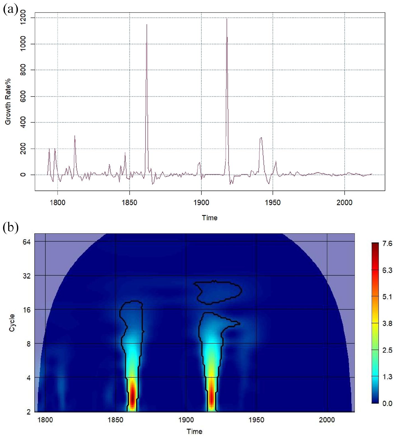
(a) U.S. Defense Spending Growth 1793–2019. (b). The Power Spectrum of U.S. Defense Spending Growth.
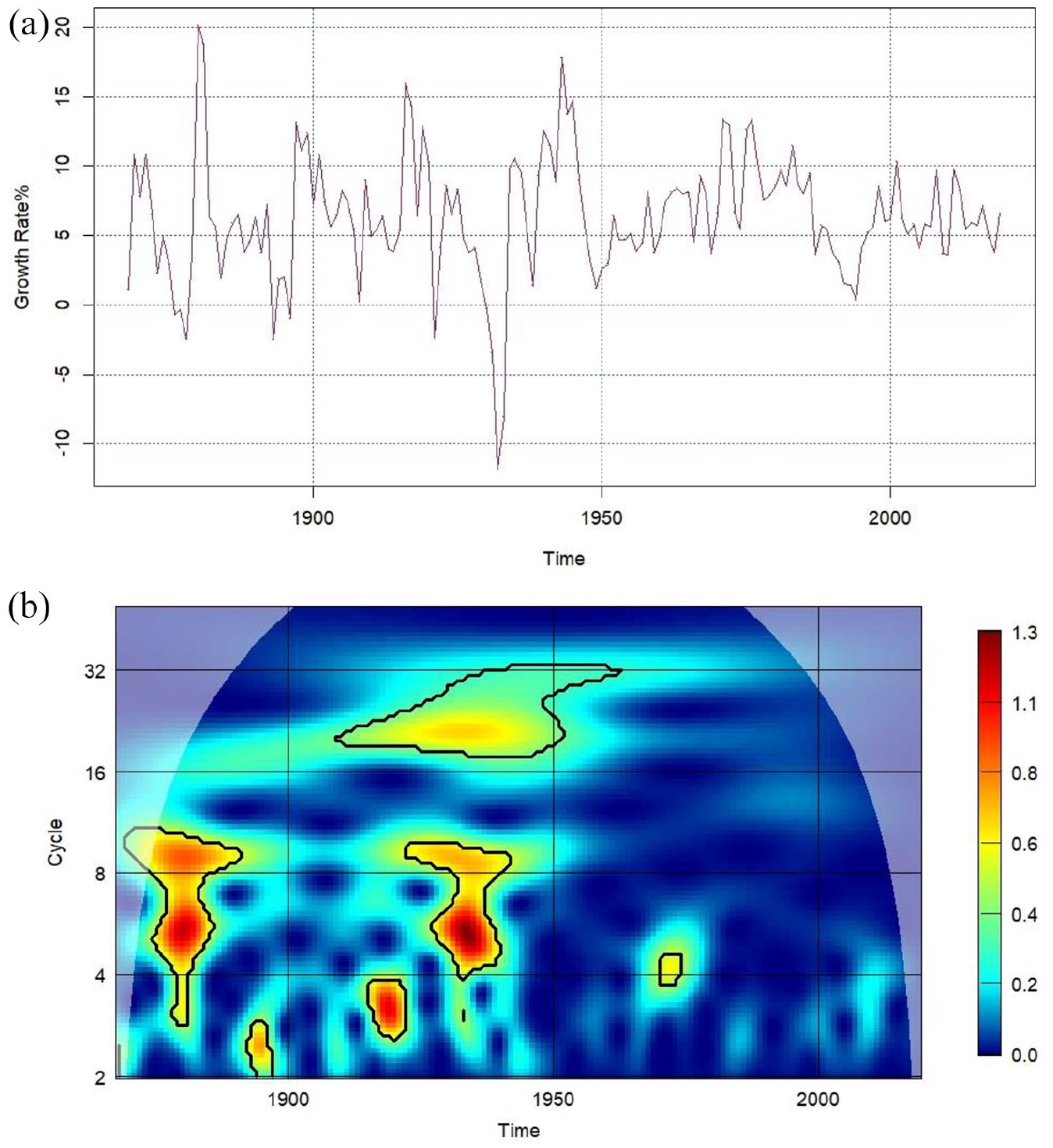
Figure 2(a) and (b) shows U.S. inflation and its power spectrum, respectively. U.S. inflation reveals frequent oscillations associated with boom-and-bust business cycles. The inflation series first amplifies itself from the Copper Panic to the end of the American Civil War. The variance in inflation then becomes stable until the U.S. entry into World War I. The two world wars and the period between them witness another cluster of inflation volatilities. A structural change seems to occur around 1950, after which a modicum of positive inflation with limited variance becomes the new norm. Although the oil crisis and early 1980s recession do spur inflation, the impact is far less compared with earlier episodes. The power spectrum, shown in Figure 2(b), confirms the above observations. From 1792 to 1870, the variance in inflation is significant at the 2- to 16-year cycles. From 1917 to 1953, the volatility of inflation is significant at the 2- to 12-year cycles and the 28- to 32-year cycles. The inflation rate is highly stable and hence insignificant for other timespans.
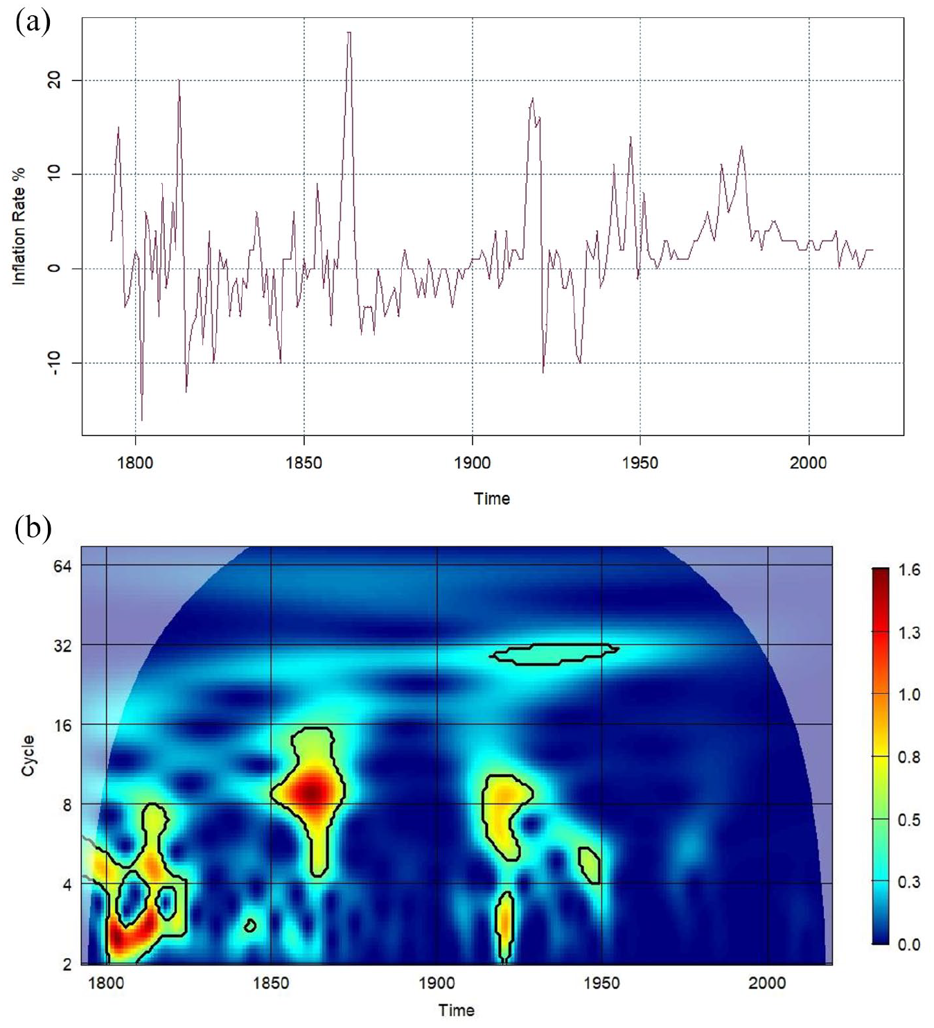
(a) U.S. Inflation Rate 1793–2019. (b) The Power Spectrum of U.S. Inflation Rate.
Figure 3 depicts the average phase angle of defense budget growth as a solid green line, the average phase angle of the inflation rate as a solid blue line, and their difference as a dashed red line, regarding four bands of cycles. The band of short cycles ranges from 2 to 5 years. The band of intermediate cycles ranges from 5 to 25 years. The band of long cycles ranges from 25 to 50 years. The band of super-long cycles includes any cycle longer than 50 years. According to Aguiar-Conraria and Soares (2014), this approach is equivalent to the approach introduced in equation (8). Thus, the method of interpretation mentioned there can be applied. In the band of short cycles, the growth of defense spending and inflation typically move in phase though antiphase movements can also be detected, and the two series frequently take turns leading each other. For the band of intermediate cycles, the two series always move in phase. The growth of defense spending leads between 1850 and 1970, between 1940 and 1960, and after 2010, while inflation leads for the rest of the time. For the long and super-long bands, the two series synchronize in an almost perfect fashion.
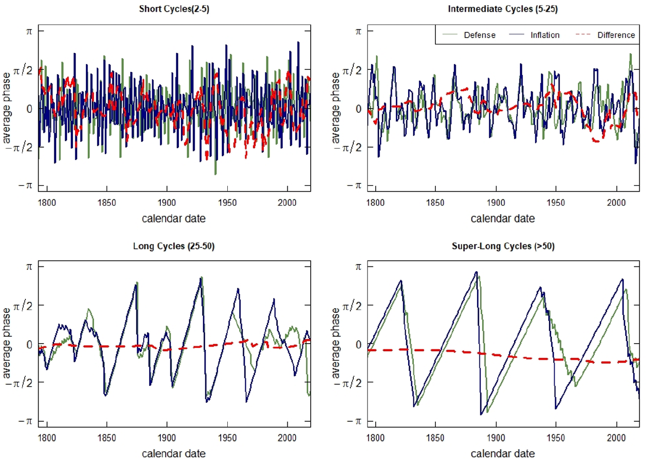
Phase Angle and Difference (U.S.).
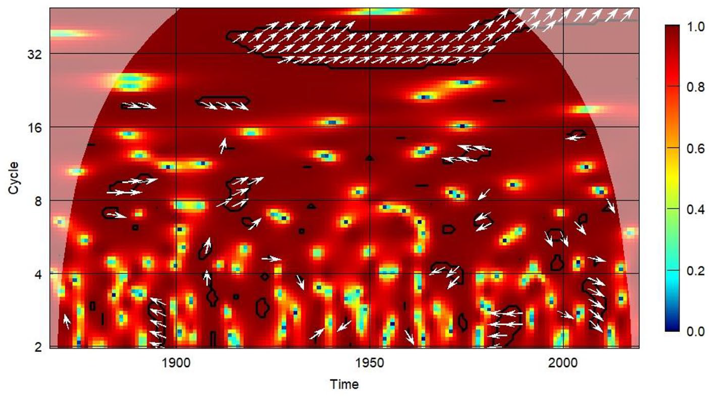
There are two major disadvantages involved in the above interpretation, however. First, we cannot test the statistical significance of the patterns detected. Second, the edge effect has been ignored. To correct for these, Figure 4 shows the wavelet coherency of defense budget growth and inflation. The contour lines again indicate the 5% level of significance, which is, in turn, decided by 5000-time Monte Carlo simulations of the red-noise process. Similar to the analyses of the power spectrum, the translucent area indicates the COI that controls for the edge effect. Arrows indicate the local phase angle of the cross-wavelet transform that is introduced by equation (8) and hence reflect the lead-lag relation between budget growth and inflation.
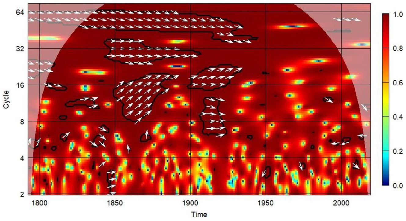
U.S. Defense-Inflation Wavelet Coherency.
According to Figure 4, the two series display a high level of coherency in both the time and frequency dimensions. In the U.S., defense budget growth and inflation can move out of phase, but that occurs only rarely and is short-lived. For cycles longer than 6 years, the two series always move in phase. The growth of defense spending leads inflation at the 2- to 4-year cycles in the 1840s, and at the 8- to 24-year cycles from 1825 to 1940. Conversely, inflation leads the growth of the defense budget at the 5- to 7-year cycles in the 1930s and at the 25- to 64-year cycles from 1925 to 1940. The results thus provide clear evidence in support of bilateral effects between defense budget growth and inflation in the U.S. It is worth noting, however, that the defense–inflation nexus disappears almost entirely after World War II. Since most of the existing empirical studies of the U.S. use data samples that cover only the Cold War era, this result helps to explain why they fail to detect robust connectivity between the two.
The Case of Britain
British defense budget growth and its power spectrum are shown in Figure 5(a) and (b), respectively. According to Figure 5(a), the second half of the eighteenth century is characterized by clustered vibrations in the dynamics of defense spending, mostly because of engagement in imperial wars. Chronologically, the three peaks in the span are associated with the Seven Years’ War, the American War of Independence, and the French Revolutionary Wars. The most pronounced changes for the entire data sample, however, come from World Wars I and II. In both cases, the British defense budget increases by more than 400%. Switching to the power spectrum, Figure 5(b) shows that the two world wars bring about statistically significant changes in the volatility of the defense budget at cycles ranging from 2 to 32 years. Although the second half of the eighteenth century witnesses considerable volatility in the growth rate of defense spending, it is not statistically significant at the 5% level.
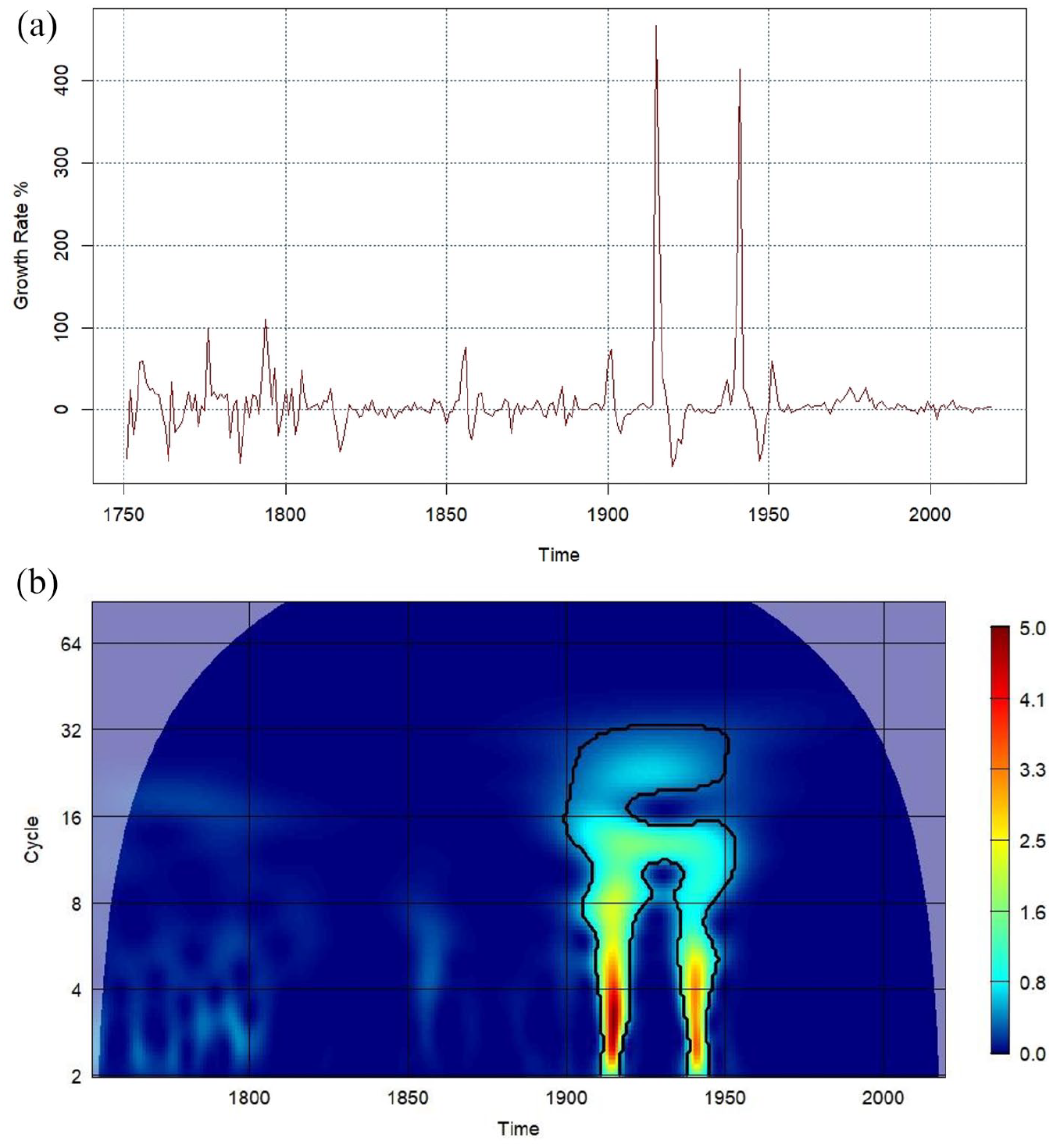
(a) British Defense Spending Growth 1751–2019. (b) The Power Spectrum of British Defense Spending Growth.
The inflation rate and its power spectrum are illustrated in Figure 6(a) and (b), respectively. The time between 1750 and 1860 witnesses frequent oscillations, among which the food shortage of 1800 and its associated riots stand out by pushing inflation up by more than 35%. The series then becomes very stable until the outbreak of World War I, which ushers in another era of clustered vibrations. In this era, the four spikes in inflation are associated chronologically with the two world wars, the oil crisis, and the 1980 recession. Finally, the recovery from that recession takes inflation back to stability until today. The power spectrum basically confirms the above observation with more information regarding the frequency domain. Before 1860, the variance in inflation is significant only for cycles shorter than 10 years. The variance in inflation during World War I is significant mostly for cycles between 7 and 14 years. After World War I, the variance in inflation is significant only for periods ranging from about 30 to 34 years. A comparison of British inflation with American inflation immediately reveals a high level of synchronization since 1870, which is likely the outcome of economic globalization.
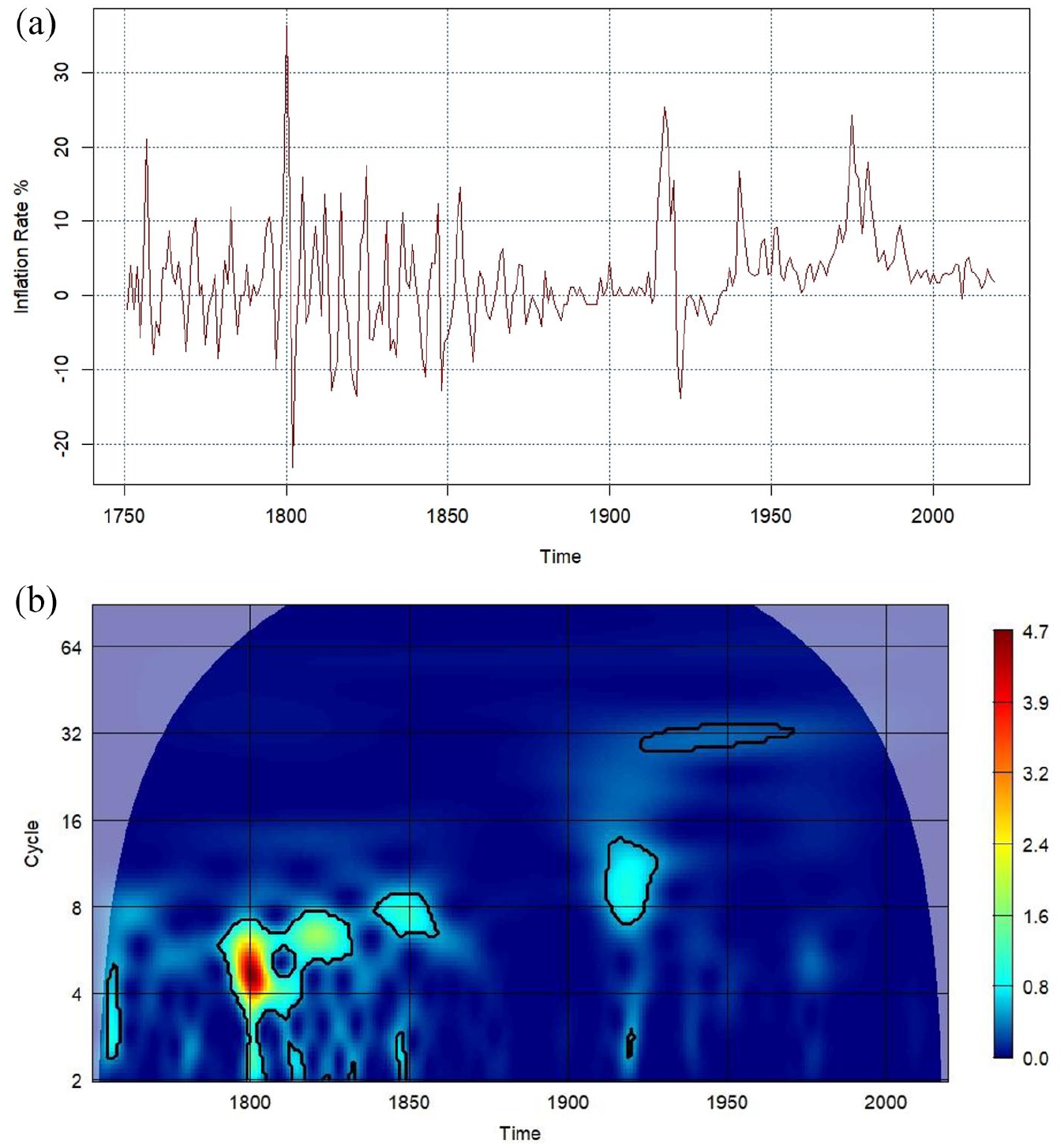
(a) British Inflation Rate 1751–2019. (b) The Power Spectrum of British Inflation Rate.
Figure 7 depicts the average phase angle of British defense budget growth, that of British inflation, and their difference as a solid green line, a solid blue line, and a dashed red line, respectively. As before, they are organized according to four bands of cycles: short (2–5 years), intermediate (5–25 years), long (25–50 years), and super long (50 years or more). Rich information regarding the lead-lag relation between British defense budget growth and inflation can be gathered. In the short term, defense budget growth and inflation are basically moving in phase except for the 1840s. The two series also take the leading role alternately. In the bands of intermediate and long cycles, the two series are always in phase. In the band of intermediate cycles, defense budget growth leads inflation between 1770 and 1800, between 1900 and 1940, in the 1970s, and after 2000. Conversely, inflation leads defense budget growth the rest of the time. In the band of long cycles, inflation leads only before 1800, while defense budget growth leads after that. In the super-long run, the two series are in phase before the 1940s, with defense budget growth leading before 1860, and inflation leading after that. They move out of phase between the 1940s and 2000, during which time defense budget growth leads inflation. After 2000, the two series move in phase again and inflation is back in the lead.
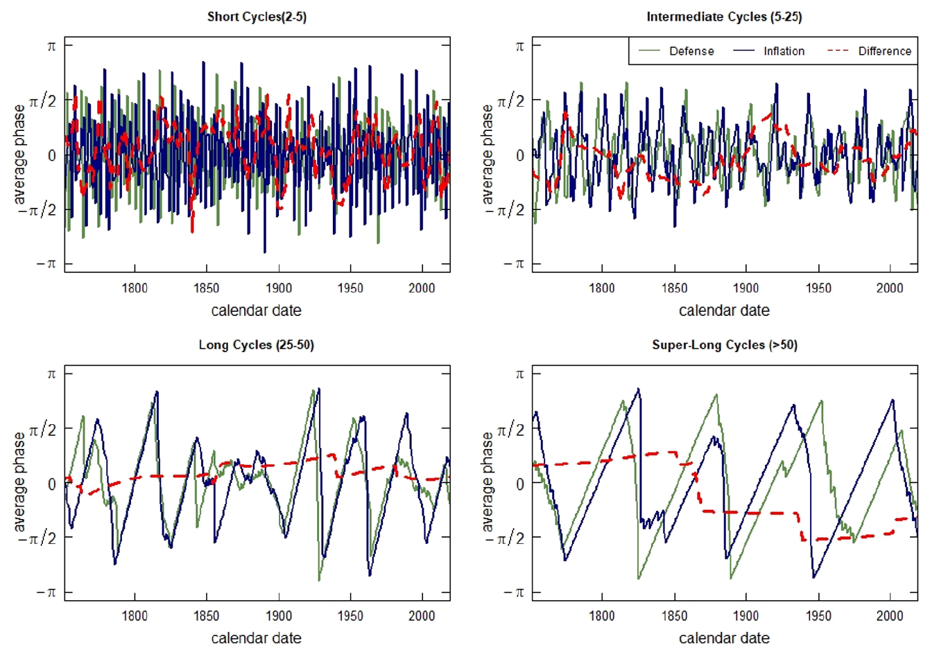
Phase Angle and Difference (Britain).
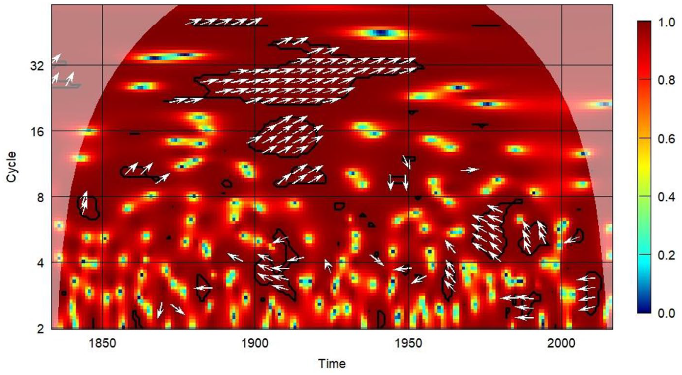
Figure 8 illustrates the wavelet coherency of defense budget growth and inflation in Britain. As mentioned before, this method of interpretation enables us to test the significance and account for the edge effect. According to the figure, defense budget growth and inflation can move out of phase. However, this occurs only in cycles shorter than 6 years. For instance, there are out-of-phase movements between 1830 and 1870. For cycles longer than 7 years, considerable evidence emerges in support of defense-driven inflation. Most noticeably, the growth of defense budgets leads inflation between 1890 and 1940 for 8- to 48-year cycles, and between 1790 and 1860 for 50- to 65-year cycles. Situations of inflation-enhanced defense budget growth can also be observed, for example, between 1840 and 1860, in the 1940s, and in the 1980s for the 7- to 20-year cycles. Note that the results are consistent with Aguiar-Conraria et al. (2012), which uses the connections between the severity of major wars and British inflation to illustrate the usefulness of bivariate wavelet analysis in dealing with periodicity, nonlinearity, and nonstationarity involved in political science data. As in the case of the U.S., there is no strong evidence for connectivity between defense budget growth and inflation in Britain from the 1950s to the 1970s for cycles of 6 or more years. As mentioned before, this result helps explain the lack of empirical evidence in support of the defense–inflation nexus. For instance, Starr et al. (1984) report no significant evidence regarding the link in the U.S. and Britain using a data sample between 1956 and 1979.
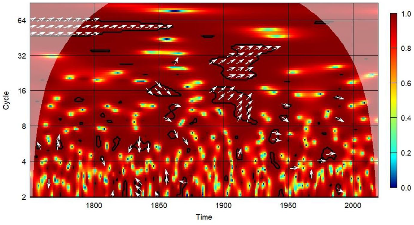
British Defense-Inflation Wavelet Coherency.
Multivariate Analysis
It is important to note that the findings reported so far are within the context of bivariate analysis. Curious readers might be interested in extending the exploration of the defense–inflation nexus to a multivariate context. For instance, monetarists believe that money supply is the fundamental driving force of inflation. For them, examining the defense–inflation nexus without considering the impact of money supply can lead to a biased estimate of the influence of the defense sector. Therefore, a relevant question is whether the established empirical patterns persist after controlling for money supply.
In the following parts of this section, we try to entertain this idea. Unfortunately, methods extending CWT in a multivariate context are still underdeveloped and face unsolved methodological hurdles. The purpose of this practice then is simply to make our discussion on the topic more complete. The preliminary results we provide do not constitute a full-fledged robustness check for the findings established in the bivariate context—an inconvenient fact for all similar research applying CWT in a multivariate context.
Pairwise Bivariate Analysis
The inclusion of money supply in our analysis brings about practical difficulties in two regards. First, the period of data availability for money supply is significantly shorter than that for defense spending or inflation. Second, money supply can be measured in several different ways and thus a choice must be made. After searching, I used the American M2 data for the period of 1868–2019 (Longtermtrends.net, 2020) and the British M0 data for 1834–2016 (The Bank of England, 2016) as the corresponding measures of the money supply. These decisions were based solely on the availability of data.
Our first strategy to examine the influence of money supply is to operate bivariate CWT analyses on the connection between money supply and inflation. Then we compare the results with those from our analyses on the nexus between defense budget growth and inflation. If the two sets of results do not overlap in the time–frequency domain, we should have more confidence in our findings on the defense–inflation nexus established in the previous section. When they do overlap, our findings become less conclusive, and additional research is needed.
Figure 9(a) and (b) shows the growth rate of U.S. M2 and its power spectrum, respectively. Both indicate a systematic change around the 1950s. Before that period, the volatility of the money supply was significant across a broad area of the time–frequency domain. From the 1950s onward, however, it was significant only at the 25- to 34-year cycles during the 1950s and 1960s and at the 4- to 5-year cycles during the 1970s.
(a) U.S. M2 Growth Rate 1868-2019. (b) The Power Spectrum of U.S. M2 Growth Rate.
Figure 10 provides the wavelet coherency between money supply and inflation in the U.S. According to the figure, the positive impact of money supply on inflation can be confirmed most conclusively in the long-run cycles above 25 years. In short and intermediate cycles, however, we can see the negative effect of inflation on the money supply since the 1950s due to the Federal Reserve’s intentional effort to curb inflation via monetary instruments. The 2008 global financial crisis clearly reversed this practice. All these observations are consistent with established economic wisdom and policy practices. A comparison of Figures 10 and 4 immediately reveals that their significant regions in the time–frequency domain do not overlap. Thus, the money supply is unlikely to influence our findings on the nexus between defense and inflation established in section “Results.” As a result, we have more confidence in the qualitative conclusion about a bilateral relationship between defense budget growth and inflation in the United States.
U.S. M2-Inflation Wavelet Coherency.
Figure 11(a) and (b) delineate the growth rate of British M0 and its power spectrum in tandem. They show that before the 1950s, the volatility of the money supply was significant only during and immediately after World War I. From the 1950s onward, it was continuously significant in long-run cycles. The most pronounced dynamics of money supply, however, came with the 2008 global financial crisis.
(a) British M0 Growth 1834–2016. (b) The Power Spectrum of British M0 Growth Rate.
Figure 12 represents the wavelet coherency between the growth rate of M0 and the inflation rate in Britain. It reconfirms what we have seen from the U.S.: the money supply does give rise to inflation, which is especially true in the long run. In shorter cycles, such as those less than 8 years, it is more often the case that the central banks use stringent monetary policy to curb inflation. However, a comparison with Figure 8 shows that there is considerable overlap between the two coherency maps for the period of 1900–1950. Thus, both defense and money supply are shown to have a positive impact on inflation. Although this finding does not necessarily disprove the defense–inflation nexus in Britain, it makes our results less conclusive and calls for further investigation.
British M0-Inflation Wavelet Coherency.
Partial Wavelet Coherency and Phase Difference
Partial wavelet coherency and partial phase difference are special tools developed to deal with analysis involving more than two series (Aguiar-Conraria and Soares, 2014). In the case of three series, we can define the partial wavelet coherency between series x and y after controlling for the impact of series z as
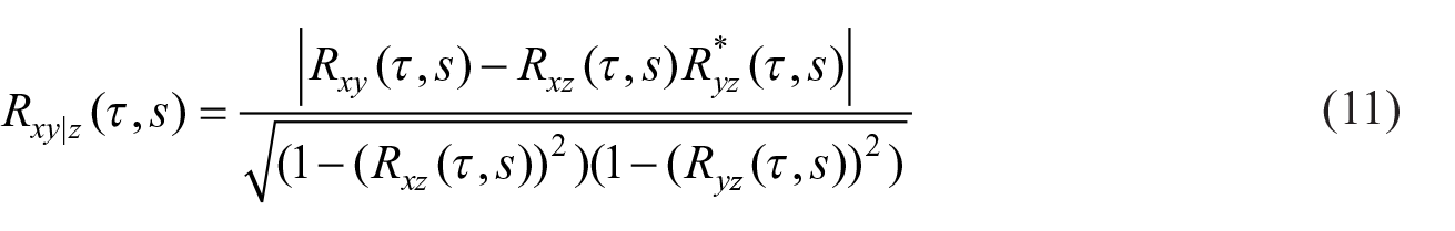
In this case, x is the growth rate of the defense budget, y is the inflation rate, and z is the growth rate of the money supply. Similarly, we can define partial phase difference as
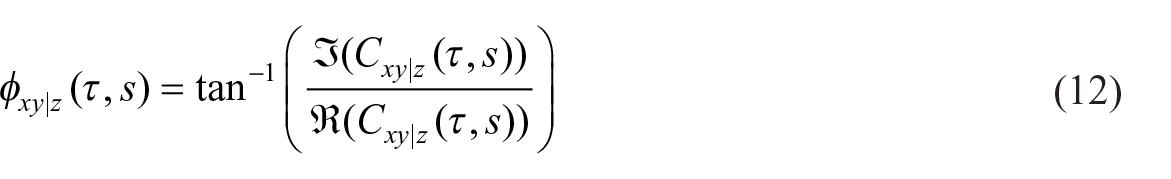
where
Figure 13 presents the partial phase difference and partial wavelet coherency for the U.S., while Figure 14 shows them for Britain. The results are obtained using the R version of the GWPackage (Aguiar-Conraria and Soares, 2014). As in bivariate analysis, we again divide cycles into four categories in the study of partial phase difference. They are short cycles (2–5 years), intermediate cycles (5–25 years), long cycles (25–50 years), and super-long cycles (50 years and above). With a few exceptions in the short cycles, both cases show that defense budget growth and inflation are always in phase after controlling for the influence of money supply. Although the growth of defense always leads to inflation in the super-long run, they alternate the leading position in intermediate and long cycles. Thus, the results support the qualitative conclusion that there is a positive bilateral effect between defense budget growth and inflation in cycles beyond the short run.
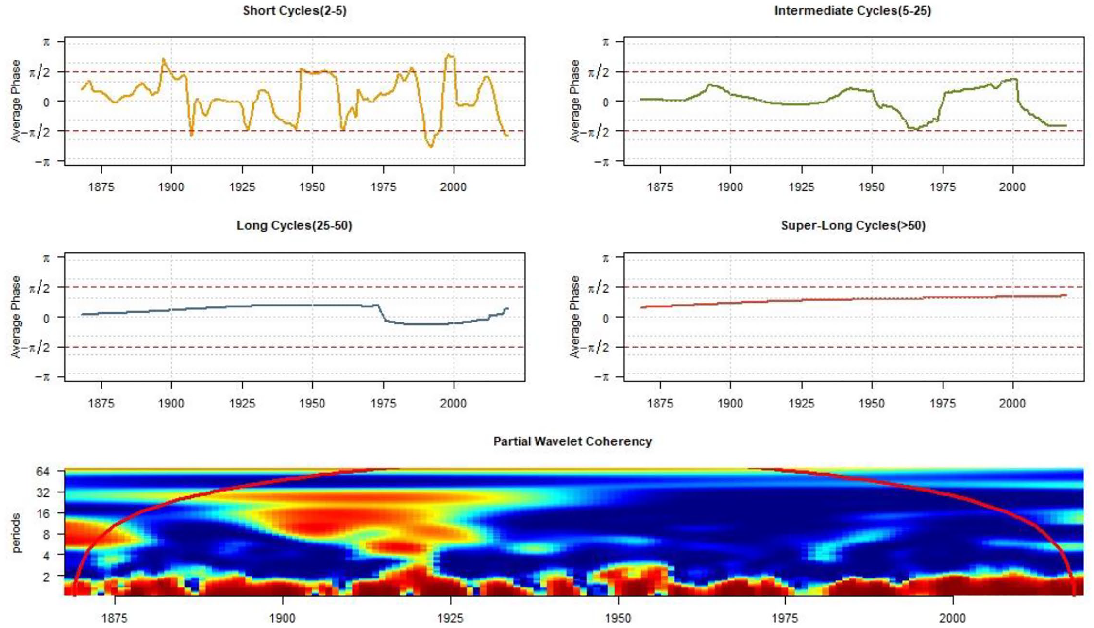
Partial Phase Difference and Partial Coherency (U.S.).
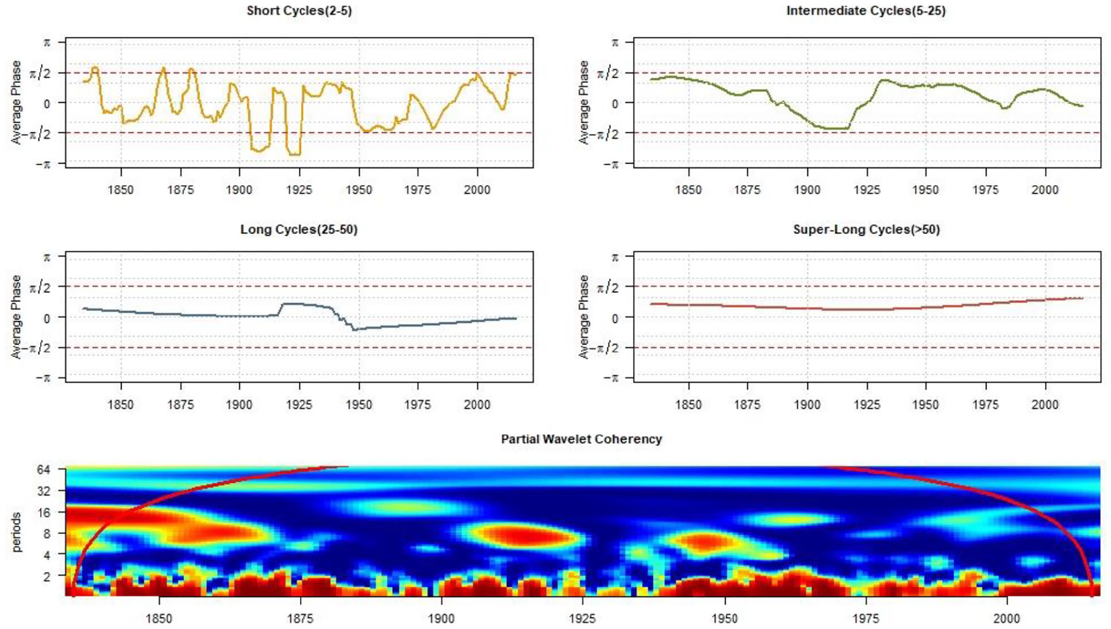
Partial Phase Difference and Partial Coherency (Britain).
Some caution, however, is needed when interpreting partial phase difference results because there is no test for statistical significance. In the bivariate context, we can rely on the significance test of wavelet coherency. Unfortunately, this strategy does not work here. Aguiar-Conraria and Soares (2014) aptly point out that no method has been developed for the significance test of partial wavelet coherency and that more research needs to be done in that direction. As a result, we cannot draw the contour lines indicating the level of significance for the graphs of partial wavelet coherency in Figures 13 and 14. In other words, although we can get estimates for the partial effects between defense budget growth and inflation after controlling for the impact of money supply, we have no clue whether such estimates are statistically significant. Obviously, this inconvenient fact considerably limits the usefulness of partial wavelet analysis in assessing the validity of our results obtained in the bivariate context.
Conclusion
This research applies continuous wavelet analysis to examine the relationship between defense budget growth and inflation in the U.S. and Britain. The results show empirical evidence in support of positive bilateral connectivity in both the cases. In the bivariate context, U.S. defense budget growth promoted inflation at 2- to 4-year cycles in the 1840s and at 8- to 24-year cycles between 1825 and 1940. Conversely, inflation accelerated defense spending growth at 5- to 7-year cycles in the 1830s and at 25- to 64-year cycles between 1825 and 1940. Similarly, British defense budget growth spurred inflation at 8- to 48-year cycles between 1890 and 1940 and at 50- to 65-year cycles between 1790 and 1860. Inflation fueled the growth of defense spending at 7- to 20-year cycles between 1840 and 1870, in the 1940s, and in the 1980s. Preliminary results from multivariate analyses are also supportive, though there is a need for further research that is contingent on advancements in the wavelet method in the direction of simulation-based significance tests.
The implications of this research are threefold. First, the current study provides supportive evidence of positive bilateral connectivity between defense spending growth and inflation in the U.S. and Britain before 1950. Since previous studies on the defense–inflation nexus in the U.S. and Britain have focused exclusively on the post–World War II period (Sahu et al., 1995; Vitaliano, 1984 Starr et al., 1984), it is unsurprising that they detected no feedback between defense budget growth and inflation. Thus, a long-term puzzle, namely, the lack of evidence from the U.S. and Britain confirming the defense–inflation nexus despite extensive theoretical writings on it, has been solved. The observation of the structural change in the 1950s, however, raises new theoretical questions. For instance, why did it happen at that moment, and what factors account for such a change? Theoretical efforts on such questions would thus be a valuable direction to pursue. One candidate variable for the disconnection is the rise of the welfare state in developed economies. A rapid rise in social spending on healthcare, education, and retirement can reduce the proportion of the government budget allocated to the defense sector (Bove et al., 2017). Another likely contributor is the establishment of the Bretton Woods financial system. As the principal promoters of the system, the U.S. and, to a lesser degree, Britain are empowered with global seigniorage that helps lessen their domestic inflation pressures (Krugman and Wells, 2015).
Second, the findings of this research have implications for the broader literature on the socioeconomic consequences of defense spending. For instance, Neoclassical and Keynesian economists have long debated the impact of expansionary military expenditure on economic growth. Keynesian economists view expansionary military spending as a way to promote overall demand and positive externalities in terms of technology, infrastructure, and human resources. Therefore, they emphasize the growth-prone effect of the defense budget. However, neoclassical economists believe that military spending easily crowds out more growth-prone investment in non-consumption sectors and, as a result, slows economic growth ceteris paribus (Deger and Sen, 1995; Ram, 1995). Because a certain level of inflation always accompanies economic growth, the lack of defense-inflation connections from the 1950s onward seems to square with empirical findings in the literature (Heo, 2010; Mintz and Huang, 1991) that question military Keynesianism and instead support the neoclassical position in today’s policymaking. Of course, applying wavelet-based methods directly to test the nexus between defense budget growth and economic growth can be a valuable direction to pursue.
The third implication of this study is methodological. Many political and economic series involve variance in both the time and frequency domains. However, traditional time-domain approaches, the powerhouse of the existing social science research on time series, focus exclusively on the former. Thus, a mismatch between the research question and the utility of methodological tools becomes inevitable. Wavelet analysis provides a powerful instrument to distill the information involved in a time-series signal into messages on the time and frequency dimensions and allows us to analyze them simultaneously. This research, along with other studies, illustrates the method’s usefulness for social scientists who treat cycles as an integral part of their research.
On this methodological front, there are three apparent extensions of the current research in the future. First, given that the strength of the defense–inflation nexus might vary from country to country, it is reasonable to consider applying the wavelet approach to explore the connectivity in states other than the U.S. and Britain. Second, given that the time–frequency perspective is a relatively new approach for social scientists, it is worth seeing whether this recent methodological stride can shed new light on critical theoretical questions. This is particularly true for topics on which social scientific theories have provided logically convincing explanations, but previous empirical research based on traditional time-domain methods has failed to provide conclusive evidence. Finally, as a relatively new research method, CWT is underdeveloped and thus limited in its current form. For instance, state-of-the-art techniques cannot operate significance tests in the multivariate context. Thus, the present results should be revisited as there are advancements in the wavelet method in the field of simulation-based significance tests.
Footnotes
Declaration of conflicting interests
The author(s) declared no potential conflicts of interest with respect to the research, authorship, and/or publication of this article.
Funding
The author(s) disclosed receipt of the following financial support for the research, authorship, and/or publication of this article: Xi’an Jiaotong-Liverpool University provides the financial support for the open-access publication of this article.