Sage Journals: Discover world-class research

Abstract

Building performance evaluation is generally carried out through a non-automated process, where computational models are iteratively built and simulated, and their energy demand is calculated. This study presents a computational tool that automates the generation of optimal building designs in respect of their Life Cycle Carbon Footprint (LCCF) and Life Cycle Costs (LCC). This is achieved by an integration of three computational concepts: (a) A designated space-allocation generative-design application, (b) Using building geometry as a parameter in NSGA-II optimization and (c) Life Cycle performance (embodied carbon and operational carbon, through the use of thermal simulations for LCCF and LCC calculation). Examining the generation of a two-storey terrace house building, located in London, UK, the study shows that a set of building parameters combinations that resulted with a pareto front of near-optimal buildings, in terms of LCCF and LCC, could be identified by using the tool. The study shows that 80% of the optimal building’s LCCF are related to the building operational stage (σ = 2), while 77% of the building’s LCC is related to the initial capital investment (σ = 2). Analysis further suggests that space heating is the largest contributor to the building’s emissions, while it has a relatively low impact on costs. Examining the optimal building in terms compliance requirements (the building with the best operational performance), the study demonstrated how this building performs poorly in terms of Life Cycle performance. The paper further presents an analysis of various life-cycle aspects, for example, a year-by-year performance breakdown, and an investigation into operational and embodied carbon emissions.

Keywords

Generative design genetic algorithms thermal simulation life cycle carbon LCA NSGA-II building performance

Introduction

The environmental efficiency of buildings has gained increasing global importance, especially since its introduction as a compliance requirement for the construction of new buildings in major economies around the world.^1,2 The improvement of the environmental efficiency of buildings is the result of a complex design process which involves passive and active design techniques and requires the consideration of various building properties, such as the building geometry (e.g. aspect ratio, orientation, spatial arrangement), envelope characteristics (e.g. build-up, window-to-wall ratio) or building systems (e.g. radiators, HVAC). While in the UK, the government policy is mainly focused on targeting operational CO₂ emissions (emissions that occur as a result of heating/cooling and electricity use), a Life Cycle Performance approach (that accounts for emissions throughout the building’s life) may be more suitable in examining the full impact of buildings on their environment.^3,4

Frameworks for evaluating the environmental efficiency of buildings have been in use across the built environment discipline since the 1990’s, and have been widely discussed in literature.^5–7 Improving buildings environmental efficiency is still regarded as a challenging task that often involves an iterative process of modelling and simulation. Currently, this iterative process is mostly carried out in a non-automated manner, where a single computational model is built and simulated, its performance assessed and changes are made to the design as required.⁸

Computer-based design is a research domain that has gained increasing interest in recent years. It relies on computational capability to automate repetitive complex processes.⁹ Advanced computational techniques (Generative design, Artificial Intelligence, optimisation, etc.) can greatly affect the architectural design process and its outcome.¹⁰ As computers become both more powerful and cheaper, and as advanced computational techniques (algorithms/software) become more commonly used, the impact of automated computational design is only expected to increase.

While advanced algorithms have been used in Architecture in the past, these were traditionally carried out mainly for formalistic purposes – achieving unique architectural forms.^11–13

Building performance optimisation frameworks have been primarily used for minimising energy consumption or optimising lighting performance, and are run mostly by programming tools such as Grasshopper, and optimisation and simulation plug-ins such as Ladybug and Honeybee.^14–16 Recently, a number of tools have been developed for optimising other performance metrics, one of which is life cycle performance. While most tools (e.g. Grasshopper’s Bombyx¹⁷ or Tortuga¹⁸), focus on the Embodied Carbon performance of buildings rather than on their entire life cycle – this is an important boost for the research of optimsiation in terms of life cycle performance. Furthermore, given that the economic value of building construction and operation is an important factor in decision-making processes in the Architecture, Engineering and Construction (AEC) sector, optimising buildings designs not only by their life cycle environmental performance, but also by their economic life cycle performance (Multi Criteria Optimisation), is of a great importance. Optimising buildings’ life cycle environmental and economic performance is still challenging, partly due to the technical difficulties in coupling various tools into a single optimsiation framework.

This paper introduces an early-stage design tool that integrates several techniques and computational frameworks (Generative design, mathematical optimisataion methods, thermal simulation and Life Cycle Performance) to optimise the design of a case study building, in terms of Life Cycle Carbon Footprint (LCCF) and Life Cycle Cost (LCC). Some of the principles that are presented in this study were tested, in a limited scope, in Schwartz,¹⁹ Schwartz et al.²⁰ and Eleftheriadis et al.,²¹ however this paper further extends those principles to:

a. Describe the complete and full framework and its sub-components in detail, and

b. Test the tool on a full-scope case study, followed by a detailed analysis of the optimal buildings’ outputs, their life cycle performance and properties.

Background: Generating optimal buildings – life-cycle performance

Attempts to use computers to automate the design of environmentally efficient buildings have been explored intensively in the last few decades. While successful frameworks have been developed and used extensively for optimising buildings in terms of daylight performance or energy consumption,¹⁶ generating optimal buildings to improve their Life Cycle Performance (carbon and cost) is still challenging. This is partly due to the need to integrate a range of analysis tools and techniques, namely: generative design, optimisation, thermal simulation and life cycle performance (environmental and economic), which are typically explored independently from one another. Integrating generative design in full life cycle performance analysis has been shown to be particularly challenging.

Despite the technological challenges, some studies presented innovative and interesting approaches for integrating some of the abovementioned techniques together. In a cornerstone study in building optimisation in terms of LCC and energy consumption, Wang et al.²² integrated optimisation methods and Life Cycle Analysis (LCA) to examine an office case study building. The study used an ASHRAE (American Society of Heating, Refrigerating and Air-Conditioning Engineers) load calculation tool to calculate operational loads, and the Athena database for calculating embodied carbon processes. While the study found optimal combination of materials and build-ups, it fell short in exploring the optimal building geometry: only the rectangular building’s orientation and its aspect ratio were manipulated. This only gave a limited scope for an automated generation of a realistic building. Furthermore, the life cycle performance in the study was measured in energy units (MJ) rather than carbon emissions (CO_2e) – a more appropriate proxy for measuring environmental impact. Ahuja et al.²³ presented a slightly different approach, using parametric building optimisers in Rhinoceros, Grasshopper and MATLAB to perform an optimisation analysis on an office case-study building. The proposed framework, however, was limited in exploring built forms, as it only examined ‘building mass’ rather than spatial arrangement and zone allocation. Furthermore, while the study analysed the buildings’ LCC, it only evaluated operational energy demand (kWh/m²/year) rather than their CO_2e. Wiberg et al.²⁴ introduced a Grasshopper/Rhino dashboard using parametric LCA models for decision-support purposes, and integrated Environmental Product Declaration (EPD) databases for embodied carbon calculation. The study, however, used an excel-based tool for calculating operational performance, and the geometric design component, again, did not consider space allocation. Grasshopper and Rhino were also used by Otovic et al.²⁵ in conjunction with EnergyPlus, to develop a real-time LCA simulation tool. The tool enabled designers to parametrically control their designs and get instant feedback about their LCCF performance, however, it only used building layouts that had been created by the users rather than created automatically. This means that not all spatial arrangements are explored, and that some optimal solutions may be missed out.

To enable a complete exploration of design variables, a LCCF and LCC optimisation framework should consist of generative design, optimisation and LCA components. The application of these in the built environment is covered below.

Mathematical optimisation

The term ‘Optimisation’ refers to the task of searching for the best solution (or solutions) out of an entire solution-set of a given problem, where a change to an input parameter can cause a change in the result.²⁶ In the built environment, where building performance is affected by various design properties (also denoted as ‘parameters’), optimisation is implemented by setting out a search mechanism that efficiently searches through multiple combinations of design properties and finds the optimal one/ones.

Computational optimisation techniques have been developed and used for various purposes since the 1960’s,²⁷ while in the built environment they have gained increasing interest since the late 2000’s.²⁸ Optimisation algorithms are used in complex parametric problems, where the search space (the entire set of possible solutions) requires significant computer resources. Most optimisation algorithms (e.g. genetic algorithms, ant colony, simulated annealing) use advanced stochastic search mechanisms – mechanisms in which some level of randomness is used to efficiently cover large search spaces in the search for desirable models. This enables the search mechanism to depict the distribution of the search space, while trying to avoid ‘local optimum’ solutions (confined areas, where no better solutions exist in the immediate proximity, while better solutions might exist further away). This is done by occasionally ‘pushing’ the search mechanism outside ‘local traps’.²⁹ Optimisation frameworks have been used in the research of the built environment in various domains:²⁸

Structural optimisation: Using optimisation algorithms to minimise the overall cost of structural elements (e.g. building slabs,^12,13 concrete bridge³⁰).

HVAC systems optimisation: Applying optimisation algorithms on the control and operation of HVAC systems to minimise their overall energy consumption, minimise their life cycle costs or maximise indoor comfort levels.^31–34

Building envelope optimisation: Using optimisation for finding the optimal wall build-ups for difference case study buildings, to reduce their environmental impacts or cost.^35–37

Life Cycle Performance optimisation: using otimisation algorithms to minimise the life cycle costs and environmental impact of new or refurbishment projects.^8,38,39

Design optimisation: Using optimisation framework to optimise simple layouts to minimise cost or energy and lighting performance,^40–42 or the appearance and structural properties of a supporting system.⁴³

Lighting: Using optimisation frameworks for optimising light levels.^44,45

A wide range of optimisation algorithms have been used in the Architecture, Engineering and Construction (AEC) sector. These include Direct Search,⁴⁶ Ant Colony,^31,32 Simulated Annealing,⁴⁷ Genetic Algorithms³⁴ and others. Covering more than 200 building optimisation studies, Nguyen et al.²⁸ show that Genetic Algorithms (GA) is the most widely used optimisation algorithm across the AEC discipline. The review also shows that among the different GA procedures, Non-Sorting Genetic Algorithms II (NSGA-II) achieved more accurate solutions, faster and more efficiently than other optimisation methods.

NSGA-II is based on the principle of Pareto Dominancy: it finds a set of solutions which are not dominated by any others: Given a series of optimsiation objectives, a solution ‘dominates’ another if it has as good results as the other solution for all objectives, and at least one result where it is better.⁴⁸ The procedure starts with the generation of an initial set (also denoted as ‘population’) of models (‘individuals’), which are the result of a random combination of design parameters. The algorithm calculates the models’ performance and identifies the non-dominated pareto solutions. It then selects some of the best-performing individuals and, based on a series of procedures inspired by the evolution theory (breeding, mutation), it mixes design parameters and creates a new set (generation) of individuals. On average, this new set is expected to perform better than the previous generation.⁴⁸ This iterative process of mixing models’ parameters and evaluation of their performance is repeated until a stopping criterion is reached (e.g. maximum number of generations).

The application of parametric design and optimisation methods is gaining increasing interest much thanks to easy-to-use platforms such as Grasshopper (a visual programming language that is a plugin for Rhinoceros 3D), Ladybug (a Grasshopper plugin for connecting models to a simulation engine) or Julia (a programming language that is used in AutoCad environments).^14–16 Other methods may include programming languages, such as Python or C#, to allow more flexibility in designing the optimisation procedures. Still, however, studies that deal with optimising spatial arrangement or building layouts for LCCF and LCC are limited.

While there is a surge in optimisation studies and application in the built environment, many of the examined tools and techniques are tailored to solve specific design problems. This is largely due to the complex and multi-layered nature of the design of the build environment, where multiple processes, stakeholders and design goals are involved. As the potential benefits of using optimisation in the design process are becoming clearer, it is expected that major software providers in the AEC will incorporate generic, flexible and easy-to-use optimisation tools within their core products.

Generative design: Within an environmental efficiency context

‘Generative design’ is a term used to describe the automation of the design process that is typically attributed to human beings only. Unlike traditional design – which focuses on the output – the focus in generative design is on procedural rules, constrains and flows that define the design process rather than the end product itself.⁴⁹

Generative design in the built environment is gaining an increasing and revived interest.⁵⁰ In its early years, though, the focus of generative design revolved mainly around innovative figurative outputs, that is, generating shapes (canopies, facades or roofs). Most notable are works by Gerber and Pantazis,¹¹ Gerber and Lin¹³ and Subhajit et al.⁵¹ However, the challenge to automatically generate building layouts that satisfy certain spatial criteria, such as minimal distances, maximum compactness, following adjacencies, etc. (also referred to as ‘the Space Allocation Problem’⁴⁹) given a set of spaces or activities still exists. Various approaches and techniques for solving the space allocation problem have been developed as early as the 1970’s.⁵² Other important work was published by Hasan et al.,³⁶ Garber³⁷ and Hillier et al.,⁵³ who presented a unique design approach using ‘shape grammars’ – a sequence of rules and conditions for space division. While various generative design techniques have been developed in recent years,⁵⁴ the automated generation of buildings with improved environmental performance is still not common.

The state-of-the-art buildings generative design techniques can be roughly divided into the following three categories:

A ‘top-down’ approach

Where space allocation is addressed from building level down to room level. A simplified generative design approach was used in various studies,^26,55–57 where simple geometric manipulations are applied on buildings’ footprint (e.g. Figure 1). In these cases, entire floors are considered as empty ‘shells’ (having no internal partitions), where the building perimeters proportions are modified. While this approach can generate a range of building designs quickly – it does not address the allocation of rooms across a building.

Figure 1.

Contour manipulation – based on.⁵⁵

Other studies^34,47,58 used the tree-map tiling algorithm diagram for dividing spaces. Tree map is a hierarchical, tree-structured procedure for sub-dividing rectangular polygons (as shown in Figure 2). Later studies introduce corridors to the designs and attempted to divide more complex spaces,^49,52 however, tree-map diagrams are only useful for specific given shapes.

Figure 2.

Shape grammar and sub-division of pre-defines spaces, based on.⁵⁸

A ‘bottom-up’ approach

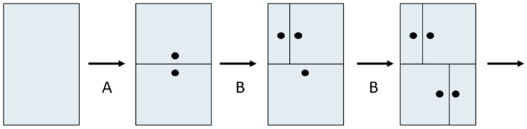
The more flexible ‘bottom-up’ techniques present a different approach by addressing the space allocation problem from the room level going up to the building level.^41,59,60 Figure 3⁴¹ shows how simple geometric manipulations are applied on an initial basic model, to generate a variety of spatial design alternatives. This approach defines a basic initial layout of four fixed and equally sized adjacent rectangular spaces and reaches a variety of building shapes by manipulating the rooms’ width and length parameters. The main weakness of this method is that the layouts are restricted to their initial fixed spatial and proximity arrangement.

Figure 3.

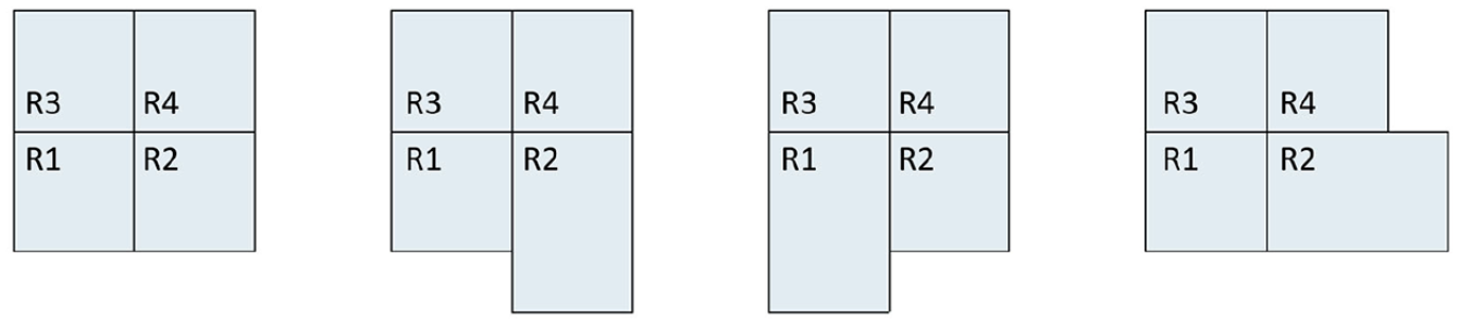
The basic starting-point layout, and some of its parametric variations, based on.⁴¹

Other ‘bottom-up’ approaches include the ‘additive space allocation’ procedure⁴⁹ – where spaces are placed based on their level of connectivity to other spaces, or the original use of a Voxel model for generating massing-layouts in a given site.⁶¹

Advanced computational frameworks

With the introduction of advanced computational techniques (Evolutionary Algorithms and Artificial Intelligence) to the built environment, advanced computational frameworks have shown increasingly promising results in generative design. Techniques for utilising advanced computational tools for generative design purposes include a heuristic distribution of spaces across a plot,⁶² the coupling of optimisation algorithms with agent-based spring-system-like frameworks,⁶³ an adaptation of a k-d tree data – a data storage method – to space planning⁵¹ or using artificial intelligence by training a Bayesian Network to generate residential buildings.¹⁰

While these approaches show increasingly promising results, some still achieved un-realistic building designs, and others suffered from the inherent limitations in machine learning algorithms, which may suggest that it is not an appropriate method for such a task: as the outcome is based on an initial man-made training set, ‘new’ or ‘innovative’ designs cannot be generated, as all designs are based on the initial batch of buildings on which the algorithm was trained.

Building performance: The Life Cycle approach

Building performance is a generic term that describes various evaluation approaches. The term aims to measure the level of efficiency of buildings, when considering various performance criteria. These might include domains such as structural stability, usability, energy efficiency, user comfort and others.

Life Cycle performance assessment captures not only the impacts of buildings operation, but also those of their construction, maintenance and processes that are related to their end of life. It is a more comprehensive approach for performance evaluation, compared to the more commonly-used energy intensity (kWh/m²/year).³

The life cycle approach has been used extensively in the research of the built environment.^64–69 It is often applied by using a comparative case study approach – where a number of design cases are evaluated, their life cycle performance is calculated, and the performance values are compared. Due to the technical complexities that are involved in a life cycle performance assessment, these studies often make a comparison between a limited number of designs. Furthermore, many of the cornerstone studies^65,68 focused on Life Cycle Energy consumption as a performance proxy. Energy-based LCA, however, may mis-represent actual emission-related impacts, as it does not identify the source of the energy that is being analysed, and energy production technologies vary significantly in their associated emissions and environmental impacts. For this reason, Life Cycle Carbon Footprint (LCCF) is regarded as a more appropriate method for evaluating the life cycle impact of buildings.

Buildings’ LCCF has been examined by several studies, looking at range of buildings types – residential, commercial, offices and others. A systematic literature review, examining the LCCF of 251 buildings from all over the world,⁷⁰ has found that the majority of buildings achieved a carbon footprint that was below 8000 kgCO₂/m²/year. Buildings with high operational-related emissions (commercial spaces, hospitals and hotels) had an average of nearly 5000 kgCO₂/m²/year, compared to 2290 kgCO₂/m²/year on average in residential buildings. Looking at the LCCF values of residential buildings in the UK and Ireland, the review found that on average, life cycle emissions were 2290 kgCO₂/m²/year and a ranged between 1020 kgCO₂/m²/year and 6200 kgCO₂/m²/year). In a recent work by the Mayor of London, the LCCF benchmark for residential buildings has been defined to be between 1050 and 1250 kgCO₂/m²/year, and the target LCCF of future buildings is planned to be set to 630–740 kgCO₂/m²/year.⁷¹

To enable a life-cycle analysis of both environmental impacts (LCCF) and economical ones (LCC), this study uses the EN 15978:2011 – Sustainability of construction works – Assessment of environmental performance of buildings – Calculation method⁴ and the BS ISO 15686-5: Building and constructed assets – Service Life Planning⁷² protocols.

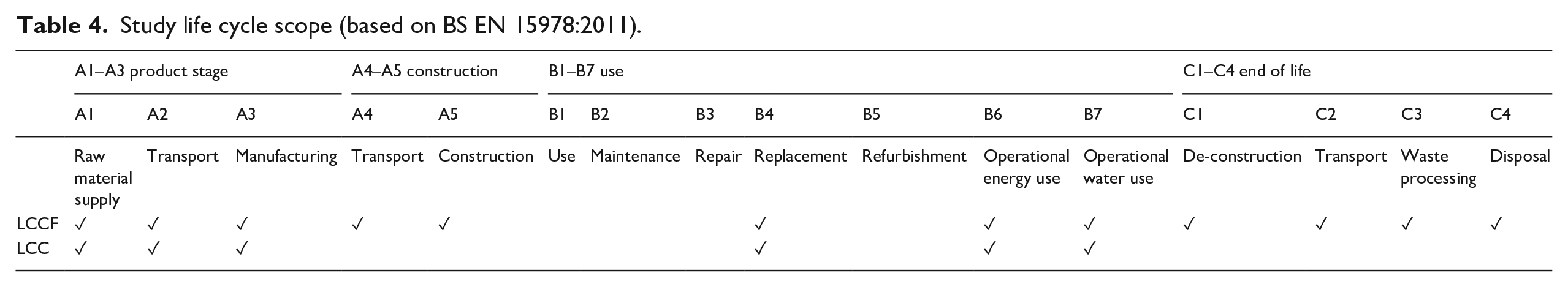
EN 15978 is one of the first standardised building life cycle calculation protocols in the world. Developed and approved by the EU, it is based on ISO standard 14040 – Environmental Management – Life Cycle Assessment and is increasingly used across the construction industry to assess life cycle impacts. In 2017, EN 15978 was officially adopted by RICS (Royal Institution of Charted Surveyors), as it may also contribute to BREEAM credits in BREEAM 2018.^73,74 The protocol defines five main stages in the life cycle of buildings, shown on Figure 4. It further uses a number of environmental categories for measuring environmental performance, based on the IPCC guidelines. However, CO_2e (CO₂ Equivalent) is often used as a proxy for translating various environmental impacts into a single comparable unit.^75,76

Figure 4.

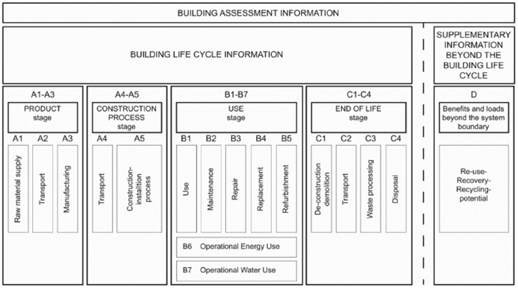
Building life cycle, according to EN 15978:2011.⁴

BS ISO 15686-5 is the protocol used by professional organisations around the world for evaluating Whole Life Costing (WLC) in the built environment, and is considered to be an industry standard.^64,65 LCC is one of the components that comprises the WLC analysis framework (as shown in Figure 5). It is often used for budgeting, cashflow forecasting and option appraisal at the project end point or at a specific point in time.^3,66,67

Figure 5.

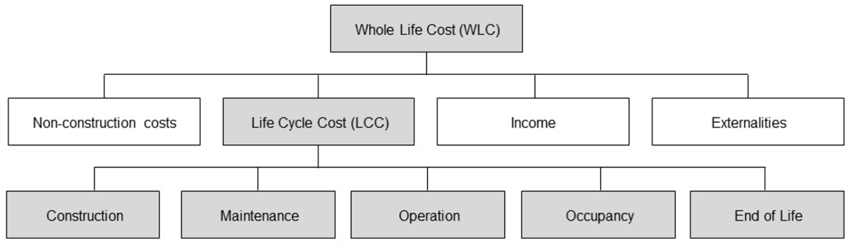
Life cycle cost (LCC) as part of whole life costing (WLC).

When cost projections are carried out, they often consider values at the time of analysis, excluding the impact of inflation on future costs. However, when future costs in different design scenarios are not of similar proportions, or when they are made in different point in time (e.g. when the cost of a future small-scale repair in the 5 years is compared against a major refurbishment in 20 years), inflation might have a more significant impact.⁷⁷ While environmental impacts are not assumed to degrade over time, the value of money might inflate or deflate as function of time. When the time factor of costs is involved, it should be expressed within the analysis. For this reason, BS ISO 15686-5 recommends calculating the ‘real value’ of money – bringing future costs to a present-day value. This should be carried out by using discounting – the process of bringing all future cost values into the current value of money.

Discounting is carried out by comparing the theoretical future return of the initial investment, assuming the money had been invested rather than spent. The difference between this prospective return and an average prospective inflation rate, expressed as percentage, is called the ‘real discount rate’.⁷⁸ The real discount rate in this study is set in accordance with the Green Book⁷⁹ and the BSRIA guide for LCC,⁷⁸ that is, 3.0%. The real discount rate is then used when calculating the overall profitability of an investment, or its Net Present Value (NPV). This is done by discounting value of future costs, minus future potential incomes (e.g. potential interest).

The Net Present Value (NPV) of a commodity is expresses by the following equation:

N P V = \sum_{i = 0}^{n} \frac{V_{i}}{{(1 + r)}^{n}}

(1)

Where:

NPV = Net Present Value

n = period of analysis in years

i = Present year

V_i = Cost in year i

r = Real discount rate

Summary: The technological challenge

The attempt to generate both life-cycle environmentally and economically optimal buildings is highly challenging as it requires the simultaneous integration of multiple processes. These are described below:

A. Computational frameworks

A.1. Generative design – the control and modification of buildings geometry-related properties (spatial arrangements, room proximities, room dimensions, etc.).

A.2. Optimisation – The search after the optimal combination of building properties to achieve the optimisation goal

B. Performance evaluation frameworks

B.1. Embodied performance evaluation – assessment of the embodied performance of each assessed design (environmental and economic).

B.2. Operational performance evaluation – assessment of the operational performance of each assessed design (environmental and economic).

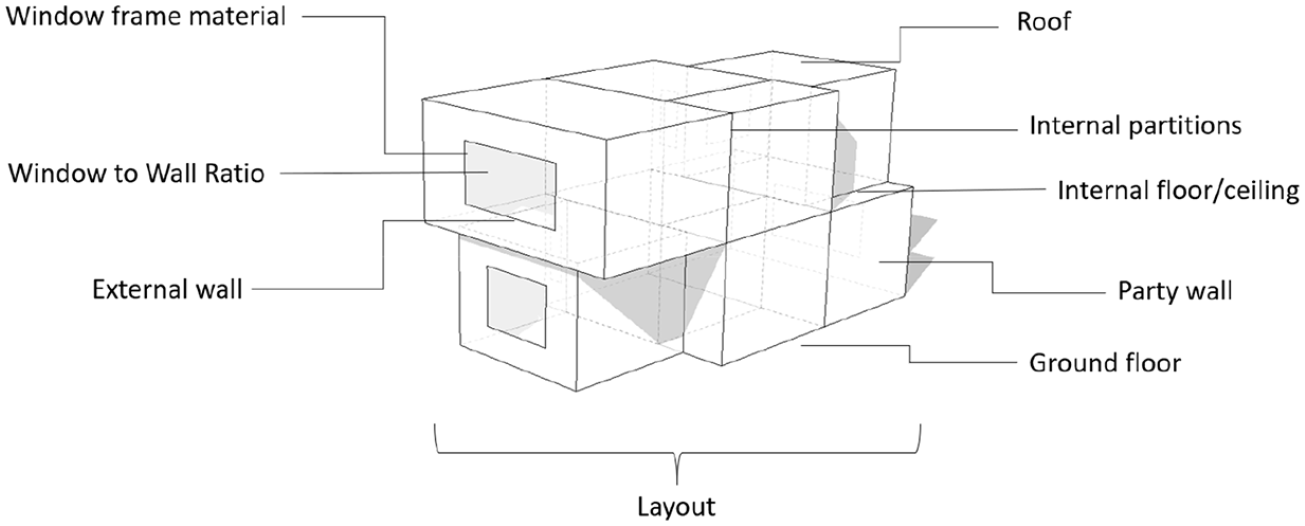
While this may suggest that two aspects of the design could be optimised separately (the buildings’ form – to minimise heat loss and material use and the building’s fabric – to minimise its life cycle impact), it was concluded that the optimisation procedure should be implemented in a single framework rather than being de-coupled into two parts, as the performance criteria in this study are cross-dependent. Separating the optimisation procedure would, therefore, not necessarily guarantee an overall optimal system (e.g. a fabric with less material and low embodied carbon will often have higher U-Value – and higher heat loss. Also, capital cost and embodied carbon are not always positively corelated – this is the case, for example, with windows frames where timber-framed windows have the lower embodied carbon, compared to uPVC and Aluminium frames, but they are also the most expensive alternative).

The proposed computational tool

To overcome these technological challenges, PLOOTO-LC (Parametric Lay-Out Organisation generaTOr – Life Cycle), a designated computational tool that integrates the above-mentioned tools and techniques was developed. PLOOTO-LC’s framework is based on existing buildings evolutionary-algorithm optimisation procedures, where models are simulated and evaluated, and building parameters are modified in a recurrent manner. This study introduces the processes that helped in the development of the tool: Firstly, while buildings forms are typically excluded from optimisation studies, this study shows how spatial arrangement, or building layout, were incorporated as a design parameter. Secondly, the study presents the development and use of an automated process for generating those buildings layouts.^19–21

To enable the full integration between generative design, thermal simulations, life cycle performance (environmental and economic) and mathematical optimisation, a designated computer programme was created. Figure 6 describes PLOOTO-LC’s components and the tools that were used to create them.

Figure 6.

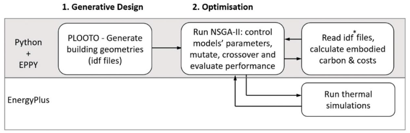
The tools and computational techniques used in PLOOTO-LC’s development.

Python 3 was used as the programming language to automate the generation of buildings layouts and models in the form of an .idf file.⁸⁰ The output of this first process was a set of EnergyPlus models, each included schedules, usage profiles and construction build-ups. EPPY (EnergyPlus Python)⁸¹ – a Python/EnergyPlus scripting language – was used in this module, as it enables easier handling of EnergyPlus files within a Python environment. Python was also used to build the NSGA-II application that controlled the evolutionary algorithm. As the optimisation criteria in this study were both embodied and operational performance, the optimisation procedure was designed to both read the idf files to get buildings’ Embodied Carbon, and run thermal simulations using EnergyPlus to get their operational-related emissions. While PLOOTO-LC’s original aim is optimising the life cycle performance of residential buildings, it can be adapted and modified to enable the optimisation of other building types.

The tool is consisted of two main components and six sub-components, as described in Figure 7. The following section describes those in detail.

Figure 7.

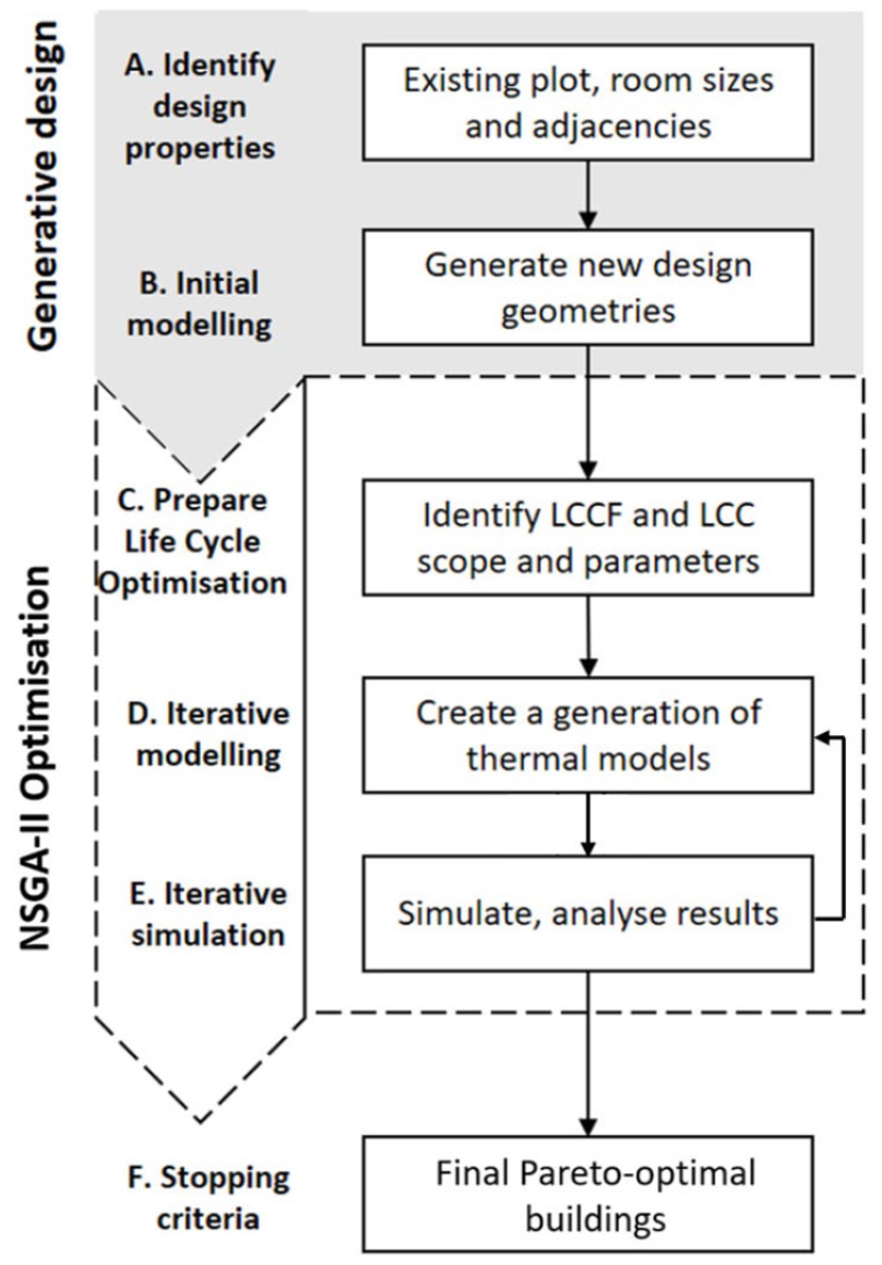
PLOOTO-LC’s computational framework.

Model generation

To enable an analysis of different building layouts’ Life cycle performance, PLOOTO-LC’s first module is responsible for the automated generation of spatial arrangements. This space allocation engine automatically generates building designs, based on heuristic principles and an initial set of user requirements (as outlined in Schwartz et al.²⁰). To enable a life cycle performance assessment, the module generates models in a suitable file format (IDF in this case) file format – which can be simulated using a thermal simulation tool (EnergyPlus).

The generation of models is the output of the following sub-processes:

A. The identification of design parameters: where various spatial design requirements are specified (e.g. plot dimensions, maximum building height, number of storeys, number of rooms at each floor, room proximities, etc.). These parameters should be chosen by the user, based on their knowledge, design intent, site limitations and building use.

B. Initial modelling: This step begins with the preparation of a ‘template’ .idf that holds pre-defined materials, build-ups, loads and schedules data. These elements follow a strict naming convention that helps allocating the appropriate properties to the different zones in the model generation process (e.g. Bedroom Occupancy Schedules begins with ‘BrOcS’. Living room Equipment Loads starts with ‘LrEqL’ etc.). No geometries nor zones are defined on these initial files, as these are generated at the next steps.

Based on the desired design properties, and on inputs from step A, models (.idf files) are then generated and saved at a designated folder. Through the model-generation process, PLOOTO-LC allocates the relevant thermal properties to each zone – based on its name and the naming convention, as described above. The names of the buildings’ different surfaces follow a similar naming strategy (e.g. the names of external exposed wall surfaces start with the initials EW, followed by a serial number. Names of internal wall surfaces start with IW followed by a serial number, etc.). This systematic naming convention assists in calculating the buildings’ embodied Carbon in the following steps.

At the end of this stage, each model holds a geometric description of a building (coordinates of the thermal zones, surface and windows) and the rooms thermal loads, usage profiles and thermal properties. Surface build-ups and materials are still not applied at this stage, as these would be assigned at the optimisation stage, ahead of the simulations.

This marks the end of the ‘model generation’ step. The .idf files are ready for the next stage: optimisation. From this stage onwards, the models’ zone geometries will not change.

Optimisation

Once the models are generated, an optimisation exercise is carried out using the spatial arrangements outputs, as well as the other user-defined building properties (thermal properties, building materials, window-to-wall-ratio, etc.) as parameters for optimisation. To implement the optimisation procedure, a designated NSGA-II (Non-Sorting Genetic Algorithms – II) application was created.

The optimisation stage is the output of the following sub-processes:

C. Preparation for Life Cycle optimisation: At this stage the scope of the study is defined, as well as the objective functions and the building parameters that are to be considered in the optimisation process.

D. Iterative modelling: Using the initial models that had been generated in sub-process B, a first generation of fully-functional models is created by assigning build-ups to the different surfaces and manipulate window-to-wall ratios.

E. Iterative simulations: At this stage the thermal simulation is carried out and the LCC/LCCF performance are calculated. Both criteria are a combination of two components: embodied and operational.

To get the embodied carbon and costs figures, models are read, and their carbon and costs values are summed: Each model (.idf) is read by the designated Python NSGA-II optimisation script. The algorithm loops through each building surface and sums the overall area of the difference building elements, based on filtering using the naming strategy as described above. The overall embodied carbon and costs of each building element is then calculated by multiplying the overall element surface area with its build-ups’ embodied carbon and costs values.

For the operational-related emissions, a thermal simulation is carried out using EnergyPlus – one of the most widely-used thermal simulation tools.²⁸ The simulated energy consumption is then translated into carbon and costs, based on energy-carbon and costs conversion factors as provided by the UK government’s National Calculation Method (NCM)⁸² and cost data⁸³ (for further details about this process, please refer to Tables 5 and 6 and section 4.2.3 – Calculating the Objective Functions). Specific modelling and calculation assumptions, including analysis boundaries, material and construction data, NPV and others are described in Tables 4 to 8.

The modelling and simulation procedures are then followed by the other optimisation processes – selection, mutation and cross-over of design properties for the next generation of models. These model characteristics are finally sent back to step D, where a new generation of models is created.

F. Once the optimisation converges – the optimisation is halted, and the pareto-optimal models are identified.

As illustrated in Figure 7, stage D of the optimisation process – iterative modelling – introduces a process without which the optimisation of the buildings in this study could not have been achieved. Here, thermal models are assembled, not only by using ‘conventional’ optimisation parameters (e.g. U-Values or Window to Wall Ratio), but also by the automatically generated geometries. This enables the optimisation procedure to evaluate the combination of different Window-to-Wall Ratio (WWR), materials and build ups ‘layered on’ various design geometries.

As NSGA-II is a heuristic-based method, to validate the application outputs and increase the confidence in the optimal or near-optimal results, three independent optimisation runs were carried out – all having the same input parameters – and their results were compared.

Implementation

Generative design

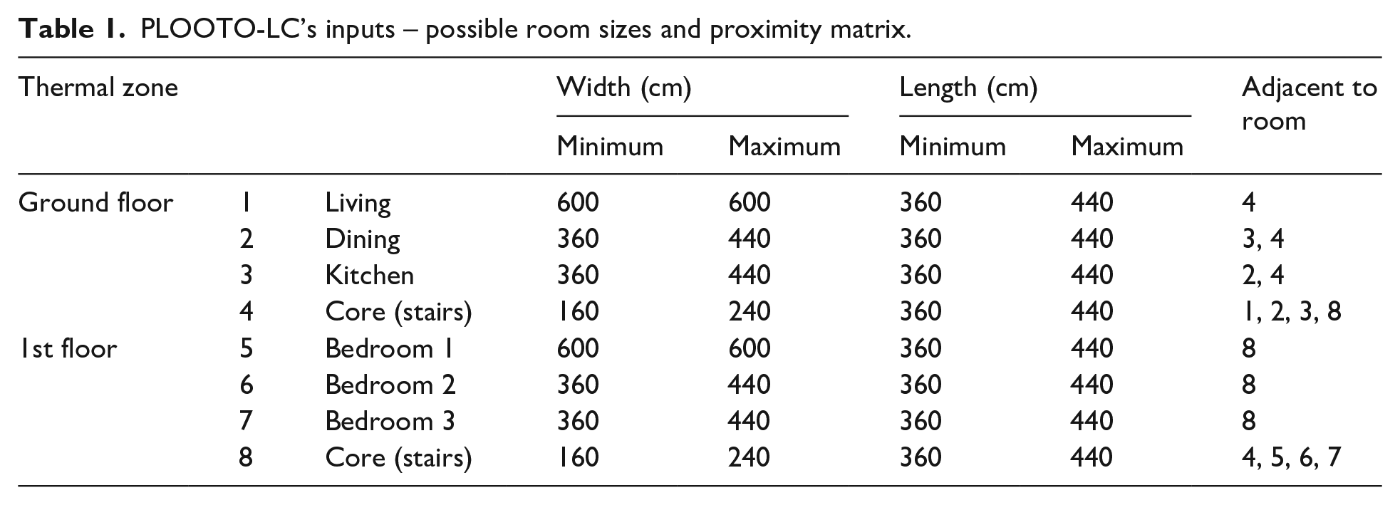
PLOOTO-LC was tested on the generation and optimisation of a two-storey terrace house building, located in London, UK. To ensure that all design outputs are similar in programme, size and volume, an initial set of design requirements was identified. Based on the classification of ‘typical’ London-based residential buildings,⁸⁴ the dimensions of the plot for the two-story generated building were set to be 6.0 × 14.6 m. A list of rooms was defined, and a room adjacency matrix was laid out (Table 1). The generative design procedure aimed to fit all rooms within the plot, as long as rooms did not exceed a re-designed range of allowed widths and lengths. Storey height was set at 3.0 m, windows could be placed on external walls only, and only when external walls were at least 0.8 m away from the edge of the plot. External walls that shared a border with adjacent plots were considered as adiabatic surfaces.

Table 1.

PLOOTO-LC’s inputs – possible room sizes and proximity matrix.

Thermal zone			Width (cm)		Length (cm)		Adjacent to room
Thermal zone			Minimum	Maximum	Minimum	Maximum	Adjacent to room
Ground floor	1	Living	600	600	360	440	4
	2	Dining	360	440	360	440	3, 4
	3	Kitchen	360	440	360	440	2, 4
	4	Core (stairs)	160	240	360	440	1, 2, 3, 8
1st floor	5	Bedroom 1	600	600	360	440	8
	6	Bedroom 2	360	440	360	440	8
	7	Bedroom 3	360	440	360	440	8
	8	Core (stairs)	160	240	360	440	4, 5, 6, 7

In the optimisation procedure, the size of each window could be examined independently of any other window (e.g. the size of a living room window could be modified and its impact on performance could be evaluated independently of the kitchen window).

To avoid model duplication or a situation in which buildings have marginals differences, a selection criteria was defined (e.g. rooms in different placements, or rooms with similar placements but at least 50 cm difference in a room’s size), and only buildings with significant difference were included in the next optimisation step. Based on the selection criteria, the tool managed to generate 32 different building forms (Figure 8).

Figure 8.

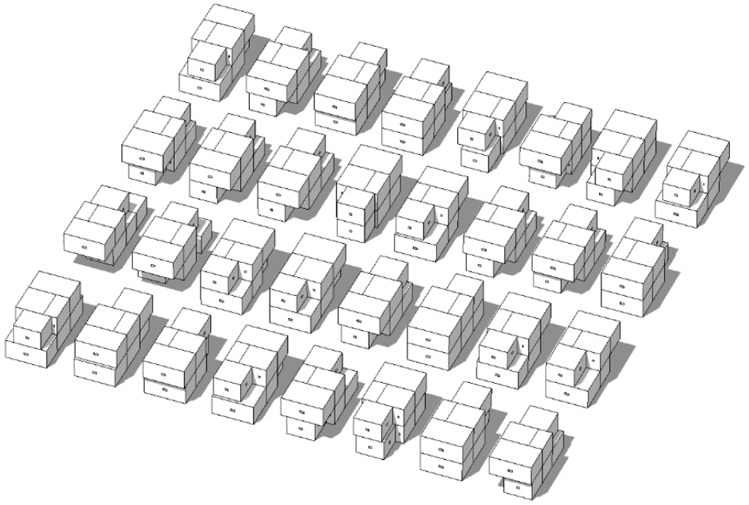
Models outputs – the 32 terrace house designs.

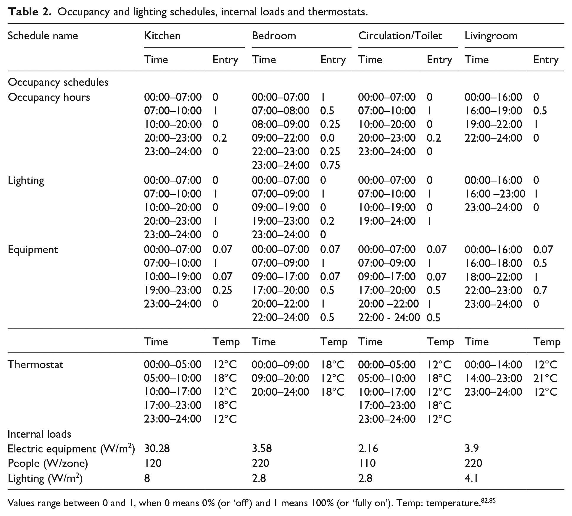
Room schedules for occupancy, internal loads and thermostats were defined per room and are shown in Table 2, based on inputs from the UK’s National Calculation Method (NCM) and CIBSE Guide A.^82,85

Table 2.

Occupancy and lighting schedules, internal loads and thermostats.

Schedule name	Kitchen		Bedroom		Circulation/Toilet		Livingroom
Schedule name	Time	Entry	Time	Entry	Time	Entry	Time	Entry
Occupancy schedules
Occupancy hours	00:00–07:00 07:00–10:00 10:00–20:00 20:00–23:00 23:00–24:00	0 1 0 0.2 0	00:00–07:00 07:00–08:00 08:00–09:00 09:00–22:00 22:00–23:00 23:00–24:00	1 0.5 0.25 0.0 0.25 0.75	00:00–07:00 07:00–10:00 10:00–20:00 20:00–23:00 23:00–24:00	0 1 0 0.2 0	00:00–16:00 16:00–19:00 19:00–22:00 22:00–24:00	0 0.5 1 0
Lighting	00:00–07:00 07:00–10:00 10:00–20:00 20:00–23:00 23:00–24:00	0 1 0 1 0	00:00–07:00 07:00–09:00 09:00–19:00 19:00–23:00 23:00–24:00	0 1 0 0.2 0	00:00–07:00 07:00–10:00 10:00–19:00 19:00–24:00	0 1 0 1	00:00–16:00 16:00 –23:00 23:00–24:00	0 1 0
Equipment	00:00–07:00 07:00–10:00 10:00–19:00 19:00–23:00 23:00–24:00	0.07 1 0.07 0.25 0	00:00–07:00 07:00–09:00 09:00–17:00 17:00–20:00 20:00–22:00 22:00–24:00	0.07 1 0.07 0.5 1 0.5	00:00–07:00 07:00–09:00 09:00–17:00 17:00–20:00 20:00 –22:00 22:00 - 24:00	0.07 1 0.07 0.5 1 0.5	00:00–16:00 16:00–18:00 18:00–22:00 22:00–23:00 23:00–24:00	0.07 0.5 1 0.7 0
	Time	Temp	Time	Temp	Time	Temp	Time	Temp
Thermostat	00:00–05:00 05:00–10:00 10:00–17:00 17:00–23:00 23:00–24:00	12°C 18°C 12°C 18°C 12°C	00:00–09:00 09:00–20:00 20:00–24:00	18°C 12°C 18°C	00:00–05:00 05:00–10:00 10:00–17:00 17:00–23:00 23:00–24:00	12°C 18°C 12°C 18°C 12°C	00:00–14:00 14:00–23:00 23:00–24:00	12°C 21°C 12°C
Internal loads
Electric equipment (W/m²)	30.28		3.58		2.16		3.9
People (W/zone)	120		220		110		220
Lighting (W/m²)	8		2.8		2.8		4.1

Values range between 0 and 1, when 0 means 0% (or ‘off’) and 1 means 100% (or ‘fully on’). Temp: temperature.^82,85

Optimisation

Optimisation set-up

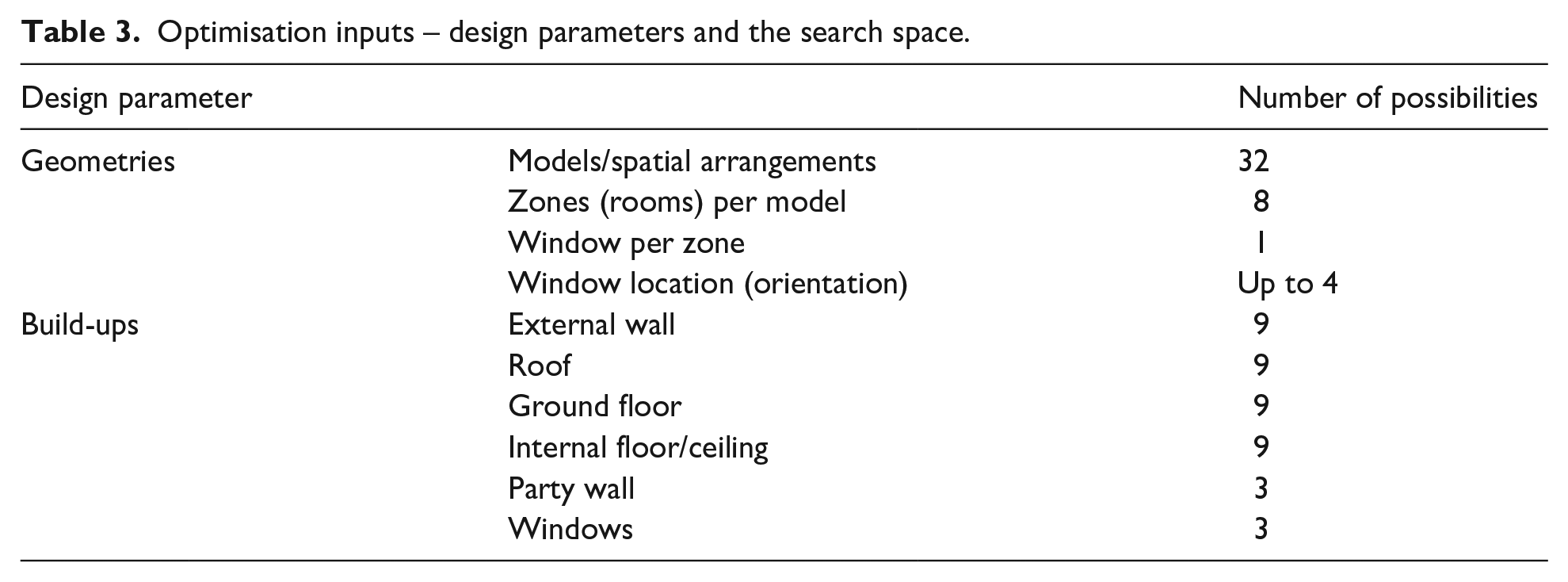
Once the models had been generated – the optimisation scope could be determined. Table 3 shows the design properties that had been chosen for the optimsiation process and the number of possible alternatives each design property had (actual building components and build-ups can be found in Table 7). Given these conditions, the search space for this study had more than 130 million possible combinations. The optimisation was executed with a uniform crossover (exchange of parents’ chromosomes where each parameter is chosen from either parent, with equal probability) of 0.8. This means that such crossover occurred for 80% of the chromosomes in each generation. The study also used a mutation rate of 0.2. This means that mutation occurred for 20% of the chromosomes in each generation: genes from the initial gene pool (as described in Tables 3 and 7) were selected randomly, using a uniformed distribution, and incorporated in the models. This is done so that new model parameters that may have been excluded in previous generations, can be introduced to the GA, as some parameters may lead to better models’ performance.

Table 3.

Optimisation inputs – design parameters and the search space.

Design parameter		Number of possibilities
Geometries	Models/spatial arrangements	32
	Zones (rooms) per model	8
	Window per zone	1
	Window location (orientation)	Up to 4
Build-ups	External wall	9
	Roof	9
	Ground floor	9
	Internal floor/ceiling	9
	Party wall	3
	Windows	3

The GA was stopped manually after 40 generations, as it was noticed that the average results per each generation had achieved similar results for more than 20 consecutive generations. Stopping criteria was manual – the procedure was stopped once convergence stabilised (as seen in section 5 –Results).

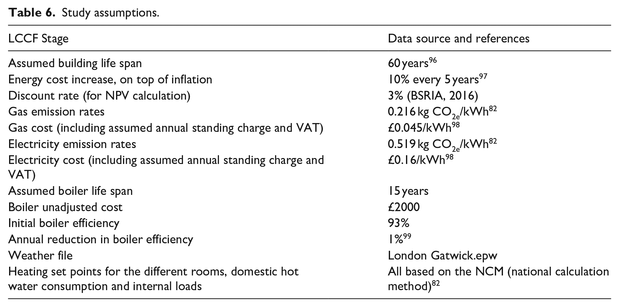
Study assumptions

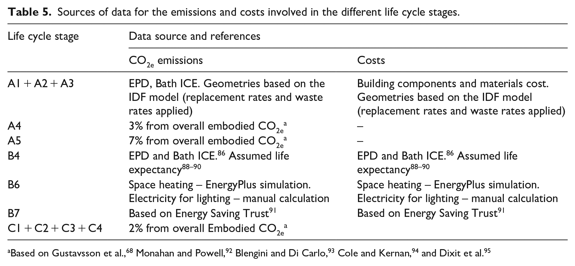
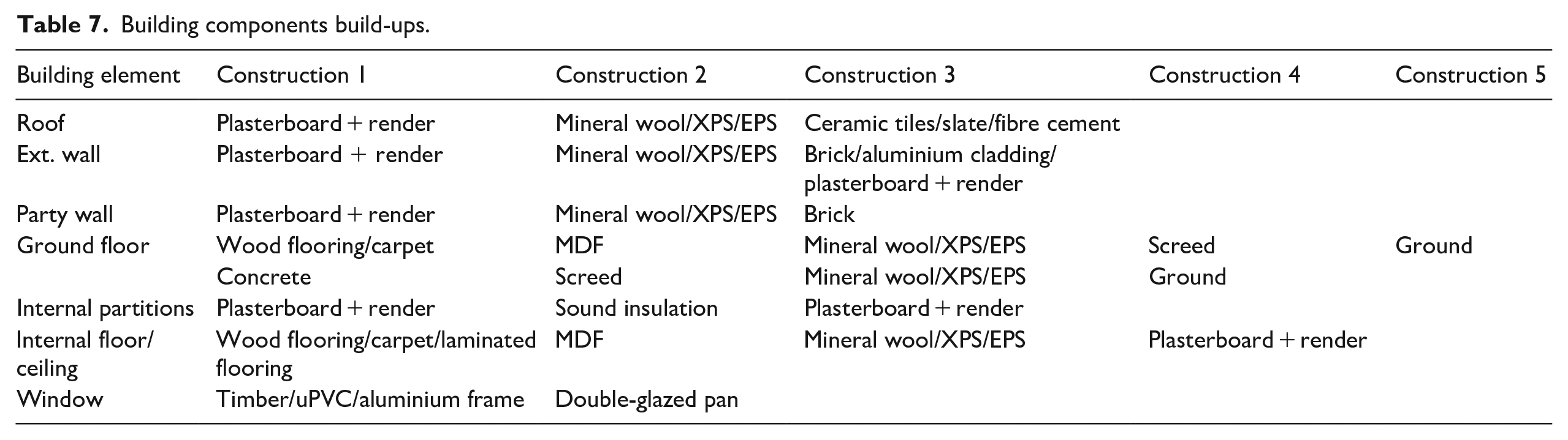
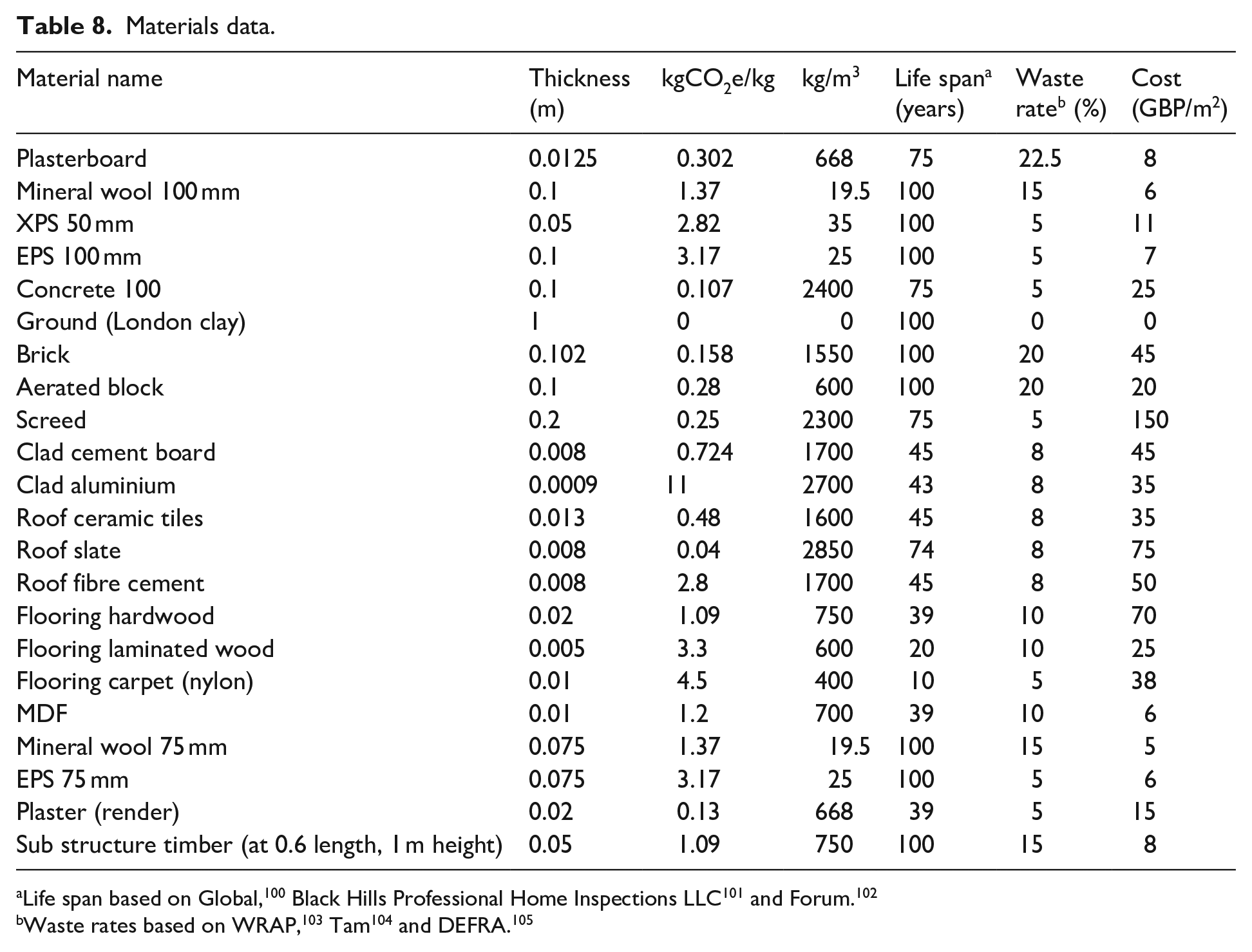
Based on BS EN 15978:2011 and BS ISO 15686-5, the case study buildings life cycle analysis scopes are described in Table 4. The calculation of Embodied CO₂ and costs were based on data from materials EPD’s, and Bath Inventory of Carbon and Energy⁸⁶ for CO₂ emissions, and on manufacturing costs and Spon’s Architects’ and Builders’ price book⁸⁷ for material costs. Sources of CO₂ emissions and cost data for the different building components and materials throughout the buildings life cycle stages are presented Tables 5 to 8 and Figure 9 below.

Table 4.

Study life cycle scope (based on BS EN 15978:2011).

	A1–A3 product stage			A4–A5 construction		B1–B7 use							C1–C4 end of life
	A1	A2	A3	A4	A5	B1	B2	B3	B4	B5	B6	B7	C1	C2	C3	C4
	Raw material supply	Transport	Manufacturing	Transport	Construction	Use	Maintenance	Repair	Replacement	Refurbishment	Operational energy use	Operational water use	De-construction	Transport	Waste processing	Disposal
LCCF	✓	✓	✓	✓	✓				✓		✓	✓	✓	✓	✓	✓
LCC	✓	✓	✓						✓		✓	✓

Table 5.

Sources of data for the emissions and costs involved in the different life cycle stages.

Life cycle stage	Data source and references
	CO_2e emissions	Costs
A1 + A2 + A3	EPD, Bath ICE. Geometries based on the IDF model (replacement rates and waste rates applied)	Building components and materials cost. Geometries based on the IDF model (replacement rates and waste rates applied)
A4	3% from overall embodied CO_2e^a	–
A5	7% from overall embodied CO_2e^a	–
B4	EPD and Bath ICE.⁸⁶ Assumed life expectancy^88–90	EPD and Bath ICE.⁸⁶ Assumed life expectancy^88–90
B6	Space heating – EnergyPlus simulation. Electricity for lighting – manual calculation	Space heating – EnergyPlus simulation. Electricity for lighting – manual calculation
B7	Based on Energy Saving Trust⁹¹	Based on Energy Saving Trust⁹¹
C1 + C2 + C3 + C4	2% from overall Embodied CO_2e^a

Based on Gustavsson et al.,⁶⁸ Monahan and Powell,⁹² Blengini and Di Carlo,⁹³ Cole and Kernan,⁹⁴ and Dixit et al.⁹⁵

Table 6.

Study assumptions.

LCCF Stage	Data source and references
Assumed building life span	60 years⁹⁶
Energy cost increase, on top of inflation	10% every 5 years⁹⁷
Discount rate (for NPV calculation)	3% (BSRIA, 2016)
Gas emission rates	0.216 kg CO_2e/kWh⁸²
Gas cost (including assumed annual standing charge and VAT)	£0.045/kWh⁹⁸
Electricity emission rates	0.519 kg CO_2e/kWh⁸²
Electricity cost (including assumed annual standing charge and VAT)	£0.16/kWh⁹⁸
Assumed boiler life span	15 years
Boiler unadjusted cost	£2000
Initial boiler efficiency	93%
Annual reduction in boiler efficiency	1%⁹⁹
Weather file	London Gatwick.epw
Heating set points for the different rooms, domestic hot water consumption and internal loads	All based on the NCM (national calculation method)⁸²

Table 7.

Building components build-ups.

Building element	Construction 1	Construction 2	Construction 3	Construction 4	Construction 5
Roof	Plasterboard + render	Mineral wool/XPS/EPS	Ceramic tiles/slate/fibre cement
Ext. wall	Plasterboard + render	Mineral wool/XPS/EPS	Brick/aluminium cladding/plasterboard + render
Party wall	Plasterboard + render	Mineral wool/XPS/EPS	Brick
Ground floor	Wood flooring/carpet	MDF	Mineral wool/XPS/EPS	Screed	Ground
Ground floor	Concrete	Screed	Mineral wool/XPS/EPS	Ground	Ground
Internal partitions	Plasterboard + render	Sound insulation	Plasterboard + render
Internal floor/ceiling	Wood flooring/carpet/laminated flooring	MDF	Mineral wool/XPS/EPS	Plasterboard + render
Window	Timber/uPVC/aluminium frame	Double-glazed pan

Table 8.

Materials data.

Material name	Thickness (m)	kgCO₂e/kg	kg/m³	Life span^a (years)	Waste rate^b (%)	Cost (GBP/m²)
Plasterboard	0.0125	0.302	668	75	22.5	8
Mineral wool 100 mm	0.1	1.37	19.5	100	15	6
XPS 50 mm	0.05	2.82	35	100	5	11
EPS 100 mm	0.1	3.17	25	100	5	7
Concrete 100	0.1	0.107	2400	75	5	25
Ground (London clay)	1	0	0	100	0	0
Brick	0.102	0.158	1550	100	20	45
Aerated block	0.1	0.28	600	100	20	20
Screed	0.2	0.25	2300	75	5	150
Clad cement board	0.008	0.724	1700	45	8	45
Clad aluminium	0.0009	11	2700	43	8	35
Roof ceramic tiles	0.013	0.48	1600	45	8	35
Roof slate	0.008	0.04	2850	74	8	75
Roof fibre cement	0.008	2.8	1700	45	8	50
Flooring hardwood	0.02	1.09	750	39	10	70
Flooring laminated wood	0.005	3.3	600	20	10	25
Flooring carpet (nylon)	0.01	4.5	400	10	5	38
MDF	0.01	1.2	700	39	10	6
Mineral wool 75 mm	0.075	1.37	19.5	100	15	5
EPS 75 mm	0.075	3.17	25	100	5	6
Plaster (render)	0.02	0.13	668	39	5	15
Sub structure timber (at 0.6 length, 1 m height)	0.05	1.09	750	100	15	8

Life span based on Global,¹⁰⁰ Black Hills Professional Home Inspections LLC¹⁰¹ and Forum.¹⁰²

Waste rates based on WRAP,¹⁰³ Tam¹⁰⁴ and DEFRA.¹⁰⁵

Figure 9.

The basic design parameters that were considered in the optimisation process.

Calculating the objective functions

The evaluation of the LCCF and LCC of each model was carried out automatically by the NSGA-II application. The programme identifies the relevant modelled building materials and their quantities, and then adds up their associated embodied CO₂ and costs factors (including CO₂ incurred by replacements, waste, transportation, etc.). Once the model thermal analysis is finished, the programme retrieves the model’s energy consumption, assigns the relevant operational CO₂ and cost values to it and adds these values to those of the embodied CO₂ and cost. Bounded by the study scope, the life cycle impact, for both CO₂ and cost, was calculated using the following formulas:

L C C F i = \sum^{} (E i p + E i t + E i c + E i r + E i o + E i e o l)

(2)

Where:

LCCFi = Life Cycle Carbon Footprint –Emissions per total floor area (kgCO_2e/m²) of the i’th model

Eip = Emissions due to overall building materials production and manufacturing

Eit = Emissions due to transport to site

Eic = Emissions due to construction works on site

Eir = Emissions due to replacements works

Eio = Emissions through the operational stage of the building (lighting, space and water heating)

Eieol = Emissions through the End of Life stage and disposal of the building

L C C i = \sum^{} (C i p + C i r + C i o)

(3)

Where:

LCCi = Life Cycle Cost – Cost per total floor area (£/m²) of the i’th model

Cip = Cost of overall building materials

Cir = Cost related to replacements works

Cio = Overall cost of the operational stage of the building (lighting, space and water heating)

The implementation of this study was carried out using UCL Legion High-Performance Computing Facility (HPC) services – an infrastructure network of a cloud computing system.¹⁰⁶ Legion enables the execution of parallel computational processes using multiple computer cores. The optimisation was executed and stopped manually after 40 generations, each consisted of 60 individuals. Using 30 threads in parallel, it took 2 h for all simulation to complete and for the optimisation to reach a convergence.

Results

Pareto-optimal models

For validation and verification purposes, three sets of optimisation runs were carried out. However, as the results were similar – only one set of outputs is shown.

Figure 10 shows the optimisation and pareto results. Figure 10(a) shows the LCCF and LCC results of the entire GA run, that is, each and every individual in the GA. It shows that overall, LCCF and LCC results ranged between 1050–1800 kgCO_2e/m² and 550–1000£/m² respectively.

Figure 10.

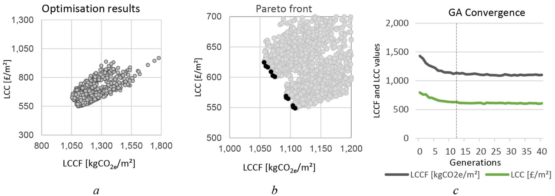
Optimisation (a) Pareto, (b) Convergence, and (c) Results.

Figure 10(b) focuses on the pareto-optimal solutions and shows that the front is consisted of 12 optimal models, with an LCCF that ranges between around 1050 and 1110 kgCO_2e/m², and LCC – between 550 and 620£/m². Compared to literature and previous studies⁷⁰ that found that the LCCF of residential buildings in the UK range between 1020 kgCO_2e/m² and 6200 kgCO_2e/m², these figures are relatively low. Still, however, this is expected as these are the LCCF values of buildings that have been optimised to reduce their LCCF as much as possible.

Figure 10(c) shows the LCCF (black) and LCC (green) average values per each generation. It shows that the first generations started with an average of around 1500 kgCO_2e/m², which, by the 10th generation, went down to around 1100 kgCO_2e/m².

All pareto-optimal models had the same building geometry (geometry number 16, as shown in detail in Figure 11) – which was proven to have the best performance of all examined geometries. This building geometry was the most efficient as it apparently has a combination of minimal volume-to-exposed-surface-area, but also cost-effective windows and construction materials. Minimising surface area both reduced heat loss and reduces construction material and its associated embodied carbon and capital costs.

Figure 11.

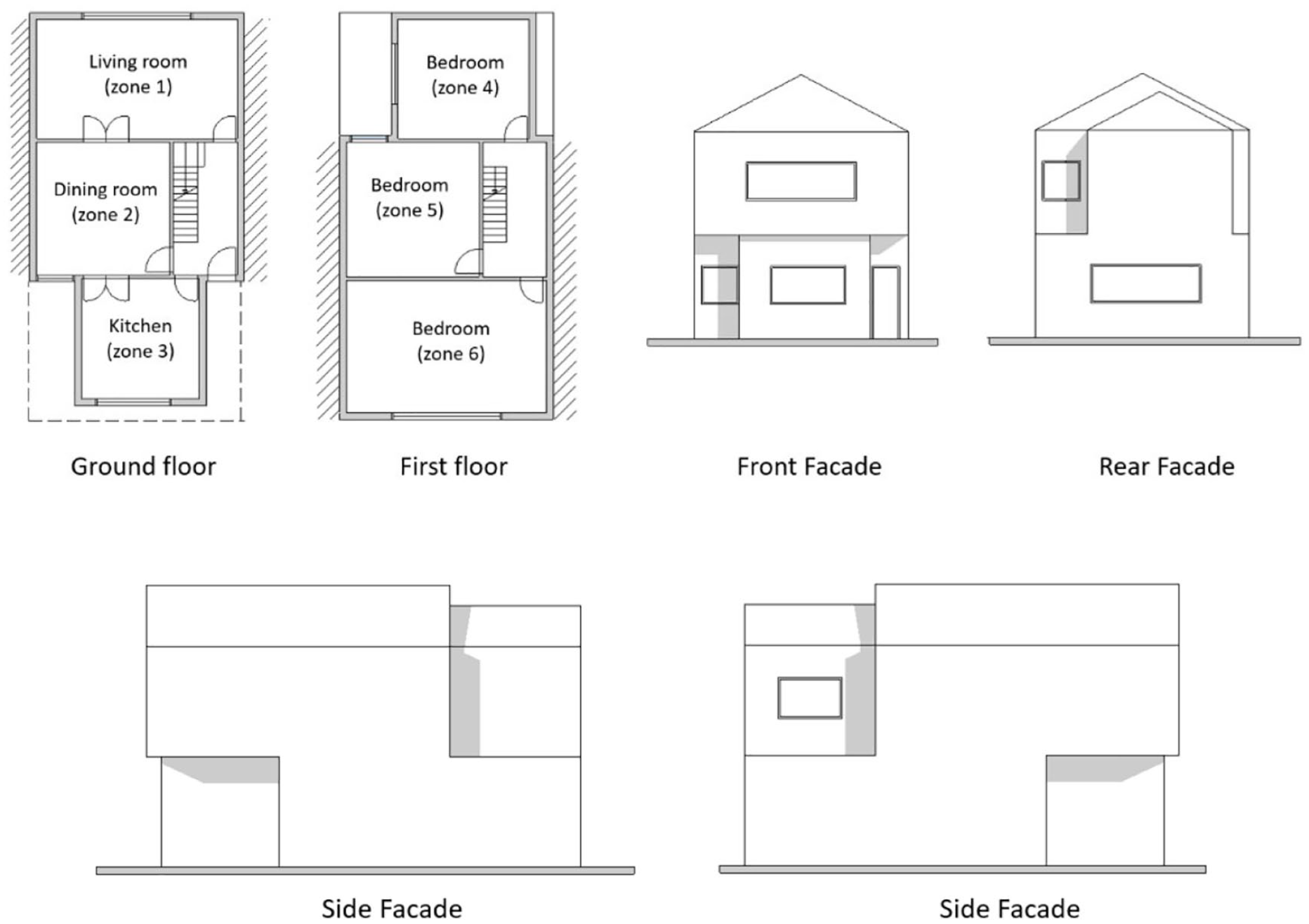
Best spatial arrangement – floor plans, elevations and thermal zones.

Furthermore, all pareto-optimal models had the same external wall, party wall and floor/ceiling build-ups, as well as window orientations (south-facing windows, whenever the layout wall orientation allowed). The pareto-front models differed however, in their roof, ground floor slab and windows constructions, as well as with the kitchen’s south-facing window-to-wall ratio.

Aggregated year-by-year emissions and costs

Next, a comparison between the aggregated annual emissions and costs of the pareto-optimal models was carried. Figure 12 shows that among the pareto-optimal models, those that had the highest LCC values also achieved minimal LCCF values, and models with lower LCC had higher LCCF values. This is because buildings with a better operational-related performance had required a higher initial investment for construction (e.g. more insultation, better windows, etc.). In some cases, more expensive construction elements had lower Embodied Carbon values, compared to the cheaper ones (timber-frame windows, for example, compared to uPVC windows). This could also contribute to the opposite relationship between LCCF and LCC throughout the buildings’ lives. Figure 12 also shows that the embodied element in the LCC (cost at year 0, or the initial investment in the buildings) equals to around 65% of the buildings’ life cycle spending, while the embodied carbon equals only around 20% of the buildings’ LCCF. This is because of the difference between the value of energy (in pounds) and its associated emissions (in CO_2e).

Figure 12.

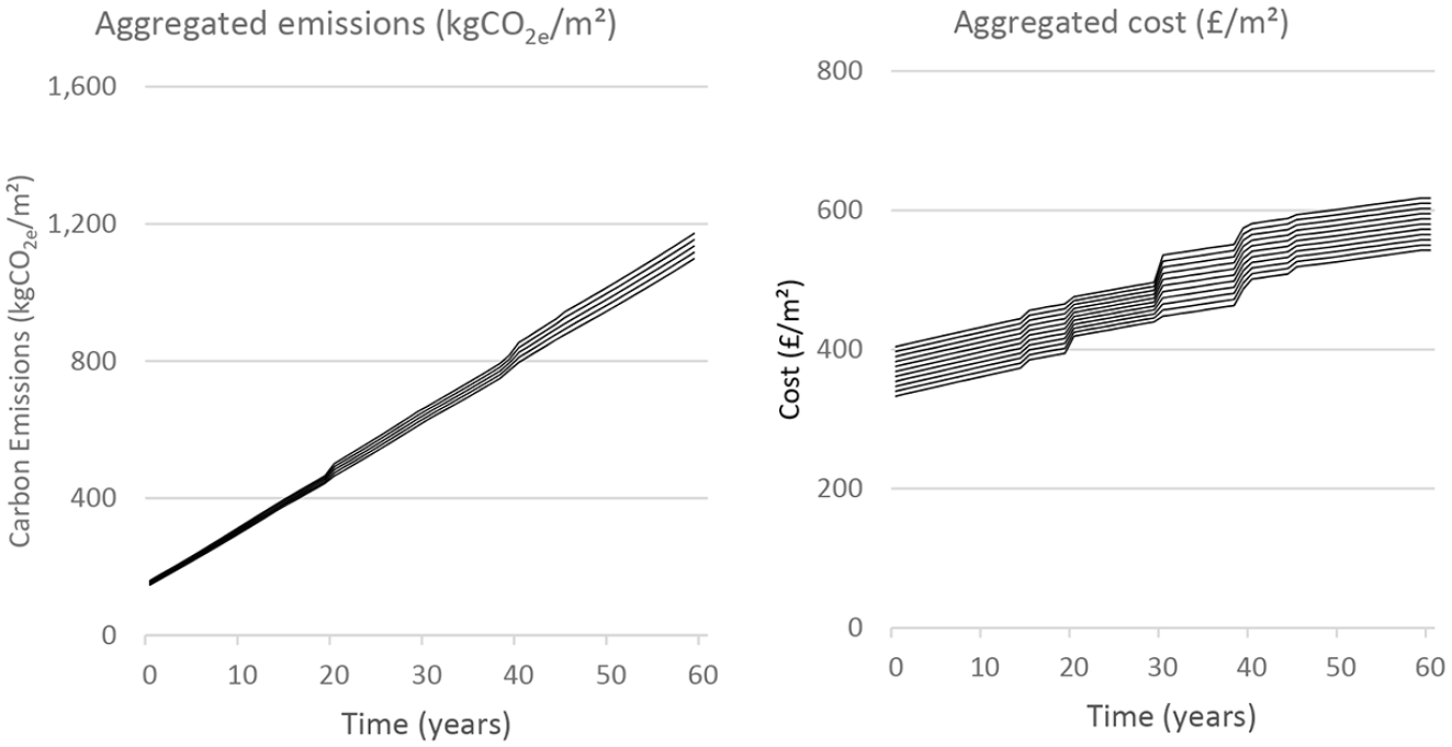
Aggregated year-by-year emissions (left) and costs (right) for the pareto front models.

Life Cycle stages

Figure 13 shows the pareto models life cycle performance, broken down by the life cycle stages (following BS EN 15978:2011). As the CO₂ emissions of a unit of energy is generally high in relation to the building’s overall initial embodied carbon, the analysis shows that the use stage (space heating, lighting and the use of domestic hot water) is the most carbon-intensive stage in the life cycle of the building, and – as expected for the climate and the typical heating fuel in London – space heating is the largest single cause of CO₂ emissions. However, when costs are examined – and since the cost of the same unit of energy in the UK is relatively low in relation to the building’s initial construction costs – results show that the operational stage has a secondary contribution to the building’s life cycle cost and that the initial investment has the highest cost throughout the building’s life. The difference between the sum of the initial capital investment and that of spending on operational purposes is also emphasised by the discounting of future spending to get the NPV of energy costs, followed by the LCC protocol as explained in section 2.3.

Figure 13.

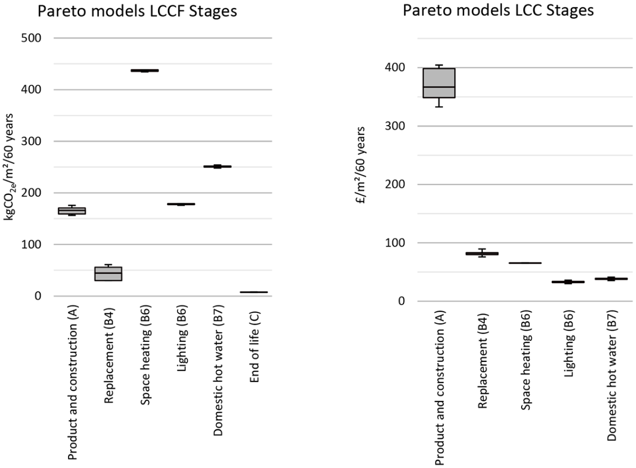
Life cycle stages break-down – LCCF (left) and LCC (right).

Proportional contribution of embodied and operational components

When comparing the ratio of the embodied and operational CO₂ and cost outputs for the optimal buildings, Figure 14 shows that the operational stage of the optimal building designs contributes most to their life cycle carbon footprint (80% on average, σ = 2). This is well aligned with the results of a systematic literature review,⁷⁰ that found that the operational stage contributes to around 75% of the LCCF, while the embodied carbon accounted for only 24%. When examining the LCC – it is the initial capital investment that has the largest part of the optimal buildings cost throughout their lives (77%, σ = 2). It is suggested that the different trend, when comparing the ratio of LCCF and LCC components, is due to the relatively low cost of the operational units (i.e. gas and electricity), compared to the cost of construction materials, whereas those operational units’ emission rates are relatively high, compared to the materials’ embodied carbon.

Figure 14.

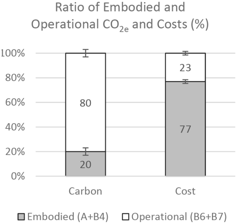
The ratio of embodied and operational emissions and costs over 60 years.

Current legislation’s life cycle performance

The framework further enabled an analysis of the life cycle performance of the optimal buildings that comply with current UK legislation. As legislation is currently focused on reducing operational consumption, an optimisation was carried out to find the optimal combination of design parameters that would lead to the building with the minimal operational energy consumption and spending on energy.

This building had the lowest possible U-Values (that were also highest in Embodied Carbon and capital costs). The LCCF and LCC of that building was then calculated and finally plotted against the Pareto-optimal solutions that were presented previously. Figure 15 shows that the optimal building, in terms of operational consumption does not result in the minimal carbon footprint or minimal life cycle costs. In fact, this building had achieved 1237 kgCO2e/m² and 668£/m², compared to an average 1094 kgCO2e/m² and 586£/m² of the pareto-optimal models. On a 60-years scale, the building that had been optimised for operational performance emits around 13% and costs around 15% more than the average pareto-optimal building (more than a total of £11,000, discounted over 60 years, or £16,500 un-discounts). This is an important finding, as it means that current policy can be improved as it does not achieve what it intends – a reduction in overall carbon emissions.

Figure 15.

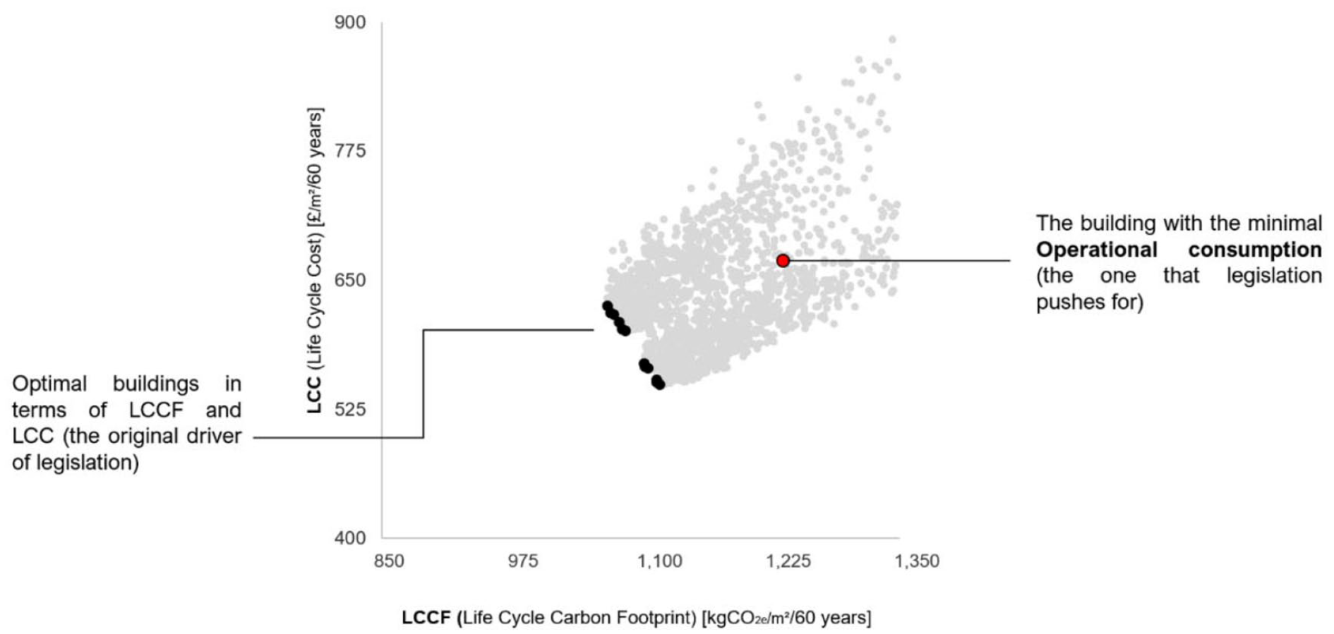
The LCCF and LCC of the optimal compliant building (operational consumption) plotted against the pareto-optimal LCCF and LCC designs, showing that the compliance has room for improvement.

As the UK government had committed to reduce CO₂ emissions in the built environment (rather than energy consumption), it is important to promote the investigation of the more comprehensive approach of ‘performance’ in buildings: exploring the contribution of the emissions that are incurred during the construction and maintenance of buildings, throughout their lives, rather than focusing on their annual energy performance solely.

Discussion and conclusions

This study has tested the implementation of a proposed computational tool for the automated generation and optimisation of building designs, in terms of their life cycle performance. The study presented an integration of generative design programming, optimisation algorithms, thermal simulations and life cycle performance evaluation frameworks (EN 15978:2011 for LCCF and BS ISO 15686-5 for LCC).

The study proposed to integrate multiple analysis methods and design techniques and successfully merged them together. PLOOTO-LC – the designated computer programme for generating buildings layouts – created a series of feasible designs based on an initial set of design criteria. These were then fed into an NSGA-II optimisation application, which automatically calculated the LCCF and LCC of each design by accessing each model, extracting surface areas, build-ups and associated CO₂ and costs, and carrying out a thermal analysis to evaluate operational CO₂ and costs. The study has shown that a set of building geometries, build-up materials and WWR combinations that results with a pareto front of near-optimal designs, in terms of LCCF and LCC, were found by using the tool.

Results show that the optimal buildings have achieved significant reductions in both LCCF and LCC, compared to existing literature. The study presented a year-by-year breakdown and a life cycle stages analysis of CO₂ emissions and cost, and showed that, in the optimal buildings, the operational-stage has the largest life cycle environmental impact, while it had a secondary impact on building life cycle cost.

The study further performed an investigation into the life cycle performance of the optimal ‘compliant’ building – the one that has the minimal operational performance. Compared to the absolute LCCF and LCC optimal buildings, though, that building achieved worse life cycle performance.

The proposed tool could potentially assist design teams, legislators and decision makers early in the design process, particularly when facing life cycle environmental and costing decisions. Though the study focused on LCCF and LCC, the computational framework can be adapted to optimise other objective criteria for example, energy intensity, operational energy consumption and others.

Limitations

Though different components of the tool have been tested and validated before,^8,20 it is acknowledged that two main types of limitations exist:

Computational application limitations: During the optimisation procedure, only the spatial arrangements that had been found by PLOOTO-LC were examined. It is noted that other spatial arrangements might exist that, when coupled with the other examined building properties, might result with better life cycle performance.

Life cycle performance limitations: This study examined buildings performance under certain settings and potential design properties (climate, orientation, construction materials, build-ups, etc.). It is acknowledged that different settings and specifications may lead to different study outcomes.

Furthermore, in calculating the embodied and operational performance of building models, this study used particular set of data (a combination of EPDs and Bath ICE) for embodied CO₂ and costs values. It is noted that when different EPDs or embodied Carbon databases are used (e.g. Bath ICE) – these values may differ.

For operational performance, the study used EnergyPlus for thermal simulation and energy consumption prediction. Although thermal simulation tools are commonly used in the research of the built environment, studies have shown that a gap exists between thermal simulation tools predictions and actual energy use.^84,107–109 Furthermore, as future weather conditions might change significantly – it is acknowledged that the predicted operational emissions figures in reality may differ from the calculated ones.

Other life-cycle-related uncertainties include various study assumptions: for example, 60 years as the assumed building life span, building components replacement rates, assumed inflation rates and others. These are limitations that are embedded within life-cycle protocols. It is also important to point out that these findings are specific for the selected location and cost parameters of the UK.

It should be noted that, however, that the flexibility of the proposed tool allows it to accommodate such future refinements. Thus, at any point, any of the input parameters (e.g. cost, embodied CO₂, life expectancy, etc.) can be modified to reflect a more accurate depiction of the model.

Lastly, while the optimisation ran for 2 h on 30 threads in parallel, this study recognises that this process is resource intensive. This means that the optimisation task could take around 8–12 h to run on a personal computer.

Future work

The development of a generative design application was a key aspect of this research. As discussed in this study, current generative design programming frameworks for architectural spatial arrangements are limited. Though the discipline of architectural generative design is not yet highly developed, it is expected that it will become more common both in academia and in practice in the future.

In that respect, PLOOTO-LC has fulfilled its aim – it resulted in a feasible and realistic set of designs. However, while the tool has shown promising results, further research and technical development of generative design approaches is needed, with a focus on their potential integration with sustainable design and engineering principles. This could lead to a more extensive research of sustainability in the built environment and to the development of a new approach to the design of efficient buildings.

Furthermore, since the scope of this study was limited to evaluating the potential of automated design of a residential building, further development is required to adapt it for application for the generation of other building uses – commercial, educational and others.

Lastly, the focus of the proposed tool is the generation of optimal buildings regarding their LCCF and LCC. Future developments are required to enable the tool to generate optimal buildings when different objectives should be account for, for example, energy use, daylight distribution, user comfort, etc.

Footnotes

Declaration of conflicting interests

The author(s) declared no potential conflicts of interest with respect to the research, authorship and/or publication of this article.

Funding

The author(s) disclosed receipt of the following financial support for the research, authorship, and/or publication of this article: This study was undertaken as part of an Engineering Doctorate (EngD) project, jointly funded by the Engineering and Physical Sciences Council (APSRC) via UCL EngD in Virtual Environments, Imaging and Visualisation (EP/G037159/1).

ORCID iD

Yair Schwartz

References

Petrullo

Jones

Morton

, et al. World green building trends 2018. SmartMarket report, Dodge Data and Analytics, USA 2018.

Lawrence

. Green building practices around the world a comparison of how sustainability and green building standards are being adopted into building construction codes within the United States and the EU. In: International conference on sustainable built environment, Hamburg, Germany, January 2012, 2017, pp. 42–51.

HM Government. Approved document L1A - conservation of fuel and poer in new dwellings. Newcastle Upon Tyne: HM Government, 2016.

BS ISO. BS EN 15978:2011 Sustainability of construction works - Assessment of environmental performance of buildings - Calculation method. BSI, 2011.

Berardi

Sustainability assessment in the construction sector: rating systems and rated buildings. Sustain Dev 2012; 20(6): 411–424.

de Castro

Mateu

Braganca

A critical analysis of building sustainability assessment methods for healthcare buildings. Environ Dev Sustain 2014; 17(6): 1381–1412.

Schwartz

Raslan

Variations in results of building energy simulation tools, and their impact on BREEAM and LEED ratings: a case study. Energy Build 2013; 62: 350–359.

Schwartz

Raslan

Mumovic

Implementing multi objective genetic algorithm for life cycle carbon footprint and life cycle cost minimisation: a building refurbishment case study. Energy 2016; 97: 58–68.

Zhang

. ‘Parallel’ EnergyPlus and the development of a parametric analysis tool. In: IBPSA conference, 2009, pp.1382–1388.

10.

Merrell

Schkufza

Koltun

Computer-generated residential building layouts. ACM Trans Graph 2010; 29(6): 1–12.

11.

Gerber

Pantazis

. A multi-agent system for facade design: a design methodology for design exploration, analysis and simulated robotic fabrication. In: Association for computer aided design in architecture (ACADIA), 2016, pp.12–23.

12.

Pantazis

Gerber

A framework for generating and evaluating façade designs using a multi-agent system approach. Int J Archit Comput 2018; 16(4): 248–270.

13.

Gerber

Lin

SE.

Designing in complexity: simulation, integration, and multidisciplinary design optimization for architecture. 2014; 90(8): 936–959.

14.

Liu

Peng

A review of performance-oriented architectural design and optimization in the context of sustainability: dividends and challenges. Sustainability 2020; 12(4): 1427.

15.

Toutou

Fikry

Mohamed

The parametric based optimization framework daylighting and energy performance in residential buildings in hot arid zone. Alexandria Eng J 2018; 57(4): 3595–3608.

16.

Sadeghipour Roudsari

Pak

Smith

, et al. Ladybug : a parametric environmental plugin for grasshopper to help designers create an environmentally-conscious design mostapha sadeghipour roudsari, Michelle Pak. In: IBPSA conference, 2013.

17.

ETH. BOMBYX. 2020, https://www.food4rhino.com/app/bombyx.

18.

Tortuga. Tortuga-LCA-grasshopper. 2020, https://www.food4rhino.com/app/tortuga-lca-grasshopper.

19.

Schwartz

An integrated thermal simulation & generative design decision support framework for the refurbishment or replacement of buildings: a life cycle performance optimisation approach, 2018.

20.

Schwartz

Raslan

Korolija

, et al. Integrated building performance optimisation: coupling parametric thermal simulation optimisation and generative spatial design programming. In: Proceedings of the 15th international conference of the international building performance simulation association, 2017, pp.1222–1229.

21.

Eleftheriadis

Schwartz

Raslan

, et al. Integrated building life cycle carbon and cost analysis embedding multiple optimisation levels Institute for Environmental Design and Engineering, University College London, London, UK Department of Civil, Environmental and Geomatic Engineering, University College London, London, UK Abstract, 2018, pp.11–12.

22.

Wang

Zmeureanu

Rivard

Applying multi-objective genetic algorithms in green building design optimization. Build Environ 2005; 40(11): 1512–1525.

23.

Ahuja

Chopson

Haymaker

, et al. Practical energy and cost optimization methods for selecting massing, materials, and technologies, 2015, pp.280–287.

24.

Wiberg

Wiik

MRK

Slåke

, et al. Life cycle assessment for zero emission buildings – a chronology of the development of a visual, dynamic and integrated approach life cycle assessment for zero emission buildings – a chronology of the development of a visual, dynamic and integrated appr. In: 1st Nordic conference on zero emission and plus energy buildings IOP, 2019.

25.

Otovic

Negendahl

Jensen

Expansion in number of parameters - simulation of energy and indoor climate in combination with LCA, no. June, 2016.

26.

Holder

The nature of mathematical programming, 2014, https://glossary.informs.org/second.php?page=nature.html.

27.

Yang

X-S.

Metaheuristic optimization, 2011, http://www.scholarpedia.org/article/Metaheuristic_Optimization.

28.

Nguyen

A-T

Reiter

Rigo

A review on simulation-based optimization methods applied to building performance analysis. Appl Energy 2014; 113: 1043–1058.

29.

Erol

Eksin

A new optimization method: Big Bang-Big Crunch. Adv Eng Softw 2006; 37(2): 106–111.

30.

Martí

González-Vidosa

Design of prestressed concrete precast pedestrian bridges by heuristic optimization. Adv Eng Softw 2010; 41(7–8): 916–922.

31.

Congradac

Kulic

HVAC system optimization with CO2 concentration control using genetic algorithms. Energy Build 2009; 41(5): 571–577.

32.

Bichiou

Krarti

Optimization of envelope and HVAC systems selection for residential buildings. Energy Build 2011; 43(12): 3373–3382.

33.

Wright

Loosemore

Farmani

Optimization of building thermal design and control by multi-criterion genetic algorithm. Energy Build 2002; 34(9): 959–972.

34.

Nassif

Kajl

Sabourin

Optimization of HVAC control system strategy using two-objective genetic algorithm. HVAC&R Res 2005; 11(3): 459–486.

35.

Islam

Jollands

Setunge

, et al. Life cycle assessment and life cycle cost implications of wall assemblages designs. Energy Build 2014; 84: 33–45.

36.

Hasan

Vuolle

Sire

Minimisation of life cycle cost of a detached house using combined simulation and optimisation. 2008; 43: 2022–2034.

37.

Garber

Optimisation stories: the impact of building information modelling on contemporary design practice. Archit Des 2009: 79(2): 6–13.

38.

Fesanghary

Asadi

Geem

ZW.

Design of low-emission and energy-efficient residential buildings using a multi-objective optimization algorithm. Build Environ 2012; 49(1): 245–250.

39.

Vasinton

Raslan

. Multi objective optimisation for the minimisation of life cycle carbon footprint and life cycle cost using NSGA II : a refurbished high-rise residential building case study. vol. 2. London: University College London (UCL), 2015.

40.

Gero

JS.

Computer-aided design by optimization in architecture. Des Stud 2006; 1(4): 227–230.

41.

Caldas

LG.

An evolution-based generative design system: using adaptation to shape architectural form. PhD Thesis, Massachusetts Institute of Technology, Cambridge, 2001.

42.

Caldas

Generation of energy-efficient architecture solutions applying GENE_ARCH: an evolution-based generative design system. Adv Eng Informatics 2008; 22(1): 59–70.

43.

Keough

Benjamin

Multi-objective optimization in architectural design. In: SpringSim’10: proceedings of the 2010 spring simulation multiconference, 2010, pp.1–8.

44.

González

Fiorito

Daylight design of office buildings: optimisation of external solar shadings by using combined simulation methods. Buildings 2015; 5: 560–580.

45.

Brown

Mueller

CT.

Design variable analysis and generation for performance-based parametric modeling in architecture. Int J Archit Comput 2019; 17: 36–52.

46.

Assiego

Larriva

Calleja Rodríguez

Cejudo López

, et al. A decision-making LCA for energy refurbishment of buildings: conditions of comfort. Energy Build 2014; 70: 333–342.

47.

Paya

Yepes

González-Vidosa

, et al. Multiobjective optimization of concrete frames by simulated annealing. Comput Civ Infrastruct Eng 2008; 23(8): 596–610.

48.

Poli

Langdon

McPhee

A field guide to genetic programming. London: Lulu Enterprises, 2008.

49.

Kalay

Architecture’s new media: principles, theories, and methods of computer-aided design. Cambridge: The MIT Press, 2004.

50.

Caetano

Santos

Leitao

Computational design in architecture: defining parametric, generative, and algorithmic design. Front Archit Res 2020; 9(2): 287–300.

51.

Subhajit

Hauck

Haymaker

, et al. Space plan generator: rapid generationn & evaluation of floor plan design options to inform decision making. In: Association for computer aided design in architecture (ACADIA), 2016.

52.

Merrell

Schkufza

Vladlen

An algorithm for exhaustive generation of building floor plans. Commun ACM 2010; 24(12): 813–825.

53.

Hillier

Leaman

Stansall

, et al. Space syntax. Environ Plan B Plan Des 1976; 3(2): 147–185.

54.

Nisztuk

Myszkowski

PB.

Usability of contemporary tools for the computational design of architectural objects: review, features evaluation and reflection. Int J Archit Comput 2018; 16(1): 58–84.

55.

Tuhus-Dubrow

Krarti

Genetic-algorithm based approach to optimize building envelope design for residential buildings. Build Environ 2010; 45(7): 1574–1581.

56.

Ali

Belal

. Multiple ant colonies optimization for load balancing in distributed systems. In: Icta’07, Hammamet, Tunisia, 2007.

57.

Ghazavi

Bonab

. Optimization of reinforced concrete retaining walls using ant colony method. In: Symposium on geotechnical safety and risk, 2011, pp.297–305.

58.

Duarte

JP.

Customizing mass housing: a discursive grammar for siza’s malgueira houses, PhD Thesis, MIT, Cambridge, 2001.

59.

Shaviv

Gali

A model for space allocation in complex buildings. Build Int 1974; 7(6): 493–518.

60.

Galle

An algorithm for exhaustive generation of building floor plans. Commun ACM 1981; 24(12): 813–825.

61.

Dillenburger

Braach

. Building design as an individual compromise between qualities and costs: a general approach for automated building generation under permanent cost and quality control. In: Tidafi

Dorta

(eds.) Joining languages, cultures and visions: CAADFutures 2009, Montreal, Canada: PUM, 2009, pp.458–471.

62.

Chatzikonstantinou

. A 3-dimensional architectural layout generation procedure for optimization applications: DC-RVD. In: Proc. 2014 eCAADe conf., vol. 1, 2014, pp.287–296.

63.

Guo

Evolutionary approach for spatial architecture layout design enhanced by an agent-based topology finding system. Front Archit Res 2017; 6(1): 53–62.

64.

van Ooteghem

. The life-cycle assessment of a single-storey retail building in Canada. Build Environ 2012; 49(1): 212–226.

65.

Ramesh

Prakash

Shukla

KK.

Life cycle energy analysis of buildings: an overview. Energy Build 2010; 42(10): 1592–1600.

66.

Tae

Shin

Kim

, et al. Life cycle environmental loads and economic efficiencies of apartment buildings built with plaster board drywall. Renew Sustain Energy Rev 2011; 15(8): 4145–4155.

67.

Ostermeyer

Wallbaum

Reuter

Multidimensional pareto optimization as an approach for site-specific building refurbishment solutions applicable for life cycle sustainability assessment. Int J Life Cycle Assess 2013; 18(9): 1762–1779.

68.

Gustavsson

Joelsson

Sathre

Life cycle primary energy use and carbon emission of an eight-storey wood-framed apartment building. Energy Build 2010; 42(2): 230–242.

69.

Eriksson

Finnveden

Ekvall

, et al. Life cycle assessment of fuels for district heating: a comparison of waste incineration, biomass- and natural gas combustion. Energy Policy 2007; 35(2): 1346–1362.

70.

Schwartz

Raslan

Mumovic

The life cycle carbon footprint of refurbished and new buildings – A systematic review of case studies. Renew Sustain Energy Rev 2018; 81: 231–241.

71.

Greater London Authority. Whole life-cycle carbon assessments guidance, 2020.

72.

BS ISO. BS ISO 15686-5:2017 Buildings and constructed assets. Service life planning. Life-cycle costing. BSI, 2017.

73.

Sturgis

Embodied and whole life carbon assessment for architects - an RBIA report, 2017.

74.

Sturgis

Whole life carbon assessment for the built environment whole life carbon assessment for the built environment - a RICS report, 2017.

75.

Forster

Ramaswamy

Artaxo

, et al. Changes in atmospheric constituents and in radiative forcing. In: Climate change 2007: the physical science basis. Contribution of working group I to the fourth assessment report of the Intergovernmental Panel on Climate Chang, 2007.

76.

Silva

. Environmental life-cycle analysis of solar systems. In: Building integrated solar thermal systems, no. March. COST - European Cooperation in Science and Technology, 2017.

77.

Gluch

Baumann

The life cycle costing (LCC) approach: a conceptual discussion of its usefulness for environmental decision-making. Build Environ 2004; 39(5): 571–580.

78.

Churcher

Tse

Life cycle costing - a BSRIA guide. Bracknell: BSRIA, 2016.

79.

Treasury

HM.

The green book - appraisal and evaluation in central government, 2011.

80.

NREL. EnergyPlus, https://energyplus.net/ (2020, accessed 23 September 2020).

81.

Python

EPPY, 2018, https://pythonhosted.org/eppy/#.

82.

NCM. National Calculation Methodology (NCM) modelling guide (for buildings other than dwellings in England), 2016.

83.

UK Power. UK power (2018) energy costs, 2018, https://www.ukpower.co.uk/home_energy/tariffs-per-unit-kwh.

84.

Oikonomou

Davies

Mavrogianni

, et al. Modelling the relative importance of the urban heat island and the thermal quality of dwellings for overheating in London. Build Environ 2012; 57: 223–238.

85.

CIBSE. Environmental design - CIBSE guide A. London: CIBSE, 2013.

86.

Hammond

Jones

. Bath ICE - Inventrory of carbon & energy V2.0. Sustainable Energy Research Team (SERT) Department of Mechanical Engineering, University of Bath, 2011.

87.

Langdon

Spon’s architects’ and builders’. Abingdon: Spons Press, 2013.

88.

EToolGlobal. Typical life expectancy of building components, 2017, http://etoolglobal.com/wp-content/uploads/2015/10/BuildingComponentLifeExpectancy.pdf.

89.

InterNACHI. Typical ‘Life Expectancy’ table for common building materials & systems, 2017.

90.

BH Home Inspections. Building materials life expectancy chart, 2018, http://www.bhhomeinspections.com/building-materials-life-expectancy-chart/.

91.

Energy Saving Trust. Measurement of domestic hot water consumption in dwellings, 2008, https://assets.publishing.service.gov.uk/government/uploads/system/uploads/attachment_data/file/48188/3147-measure-domestic-hot-water-consump.pdf.

92.

Monahan

Powell

JC.

An embodied carbon and energy analysis of modern methods of construction in housing: a case study using a lifecycle assessment framework. Energy Build 2011; 43(1): 179–188.

93.

Blengini

Di Carlo

The changing role of life cycle phases, subsystems and materials in the LCA of low energy buildings. Energy Build 2010; 42(6): 869–880.

94.

Cole

Kernan

PC.

Life-cycle energy use in office buildings. Build Environ 1996; 31(4): 307–317.

95.

Dixit

Fernández-Solís

Lavy

, et al. Identification of parameters for embodied energy measurement: a literature review. Energy Build 2010; 42(8): 1238–1247.

96.

BRE. The green guide to specification: an environmental profiling system for building materials and components, 2009.

97.

Churcher

Life cycle assessment - a BSRIA guide, 2013, https://www.bsria.co.uk/download/product/?file=zHACoSBB060%3D.

98.

UK Power. Energy costs, 2017, https://www.ukpower.co.uk/home_energy/tariffs-per-unit-kwh.

99.

Pasi

Muller

. Investigating the impact of boiler aging in replacement decision. In: ACEEE summer study on energy efficiency in industry, 2007.

100.

Global

. Typical life expectancy of building components, http://etoolglobal.com/wp-content/uploads/2015/10/BuildingComponentLifeExpectancy.pdf.

101.

Black Hills Professional Home Inspections LLC. Building materials life expectancy chart, https://www.bhhomeinspections.com/building-materials-life-expectancy-chart/.

102.

Forum

CL.

Recommended guidelines for building component lifespans in whole building life cycle assessment, 2018, pp.1–4.

103.

WRAP. Assessing the costs and benefits of reducing waste in construction cross-sector comparison, 2009.

104.

Tam

VWY

. Rate of reusable and recyclable waste in construction. Open Waste Manag J 2011; 4: 28–32.

105.

DEFRA. UK statistics on waste, 2019, https://assets.publishing.service.gov.uk/government/uploads/system/uploads/attachment_data/file/784263/UK_Statistics_on_Waste_statistical_notice_March_2019_rev_FINAL.pdf.

106.

UCL. Legion architecture, 2020, https://github-pages.ucl.ac.uk/RCPSTrainingMaterials/HPCandHTCusingLegion/3_legion_overview.html (accessed 23 September 2020).

107.

Van Dronkelaar

Dowson

Burman

, et al. A review of the energy performance gap and its underlying causes in non-domestic buildings. Front Mech Eng 2016; 1(January): 1–14.

108.

Raslan

Davies

Results variability in accredited building energy performance compliance demonstration software in the UK: an inter-model comparative study. J Build Perform Simul 2010; 3(1): 63–85.

109.

Calleja Rodríguez

Carrillo Andrés

Domínguez Muñoz

, et al. Uncertainties and sensitivity analysis in building energy simulation using macroparameters. Energy Build 2013; 67: 79–87.

A decision support tool for building design: An integrated generative design,optimisation and life cycle performance approach

Abstract

Keywords

Introduction

Background: Generating optimal buildings – life-cycle performance

Mathematical optimisation

Generative design: Within an environmental efficiency context

A ‘top-down’ approach

A ‘bottom-up’ approach

Advanced computational frameworks

Building performance: The Life Cycle approach

Summary: The technological challenge

The proposed computational tool

Model generation

Optimisation

Implementation

Generative design

Optimisation

Optimisation set-up

Study assumptions

Calculating the objective functions

Results

Pareto-optimal models

Aggregated year-by-year emissions and costs

Life Cycle stages

Proportional contribution of embodied and operational components

Current legislation’s life cycle performance

Discussion and conclusions

Limitations

Future work

Footnotes

Declaration of conflicting interests

Funding

ORCID iD

References