Sage Journals: Discover world-class research

Abstract

In this study, we employ a newly developed time series econometric approach to investigate the development in crime rates in various members states of the European Union (EU) between 1968 and 2019. We propose a panel data model with stochastically time-varying factors that also includes country-specific effects. This model enables us to evaluate the existence of a common EU crime trend, including a crime drop, to describe how individual countries depart from this common trend, and to estimate its association with macroeconomic and demographic explanatory variables. To have an equivocal measure of crime over the countries for the period of interest, we use homicide rates based on the Mortality Database from the World Health Organization. Results confirm the presence of a crime drop in the EU, be it stronger in Western EU countries than in Eastern EU countries. We also find that economic conditions explain a small portion of the crime trends in the EU; with macroeconomic activity (economic growth) being more relevant for Eastern EU countries, and macroeconomic performance (welfare growth) for Western EU countries. The young adult ratio (share of 25- to 34-year-olds in the total population) substantially explains the crime trend and drop in Western EU countries only. Our findings illustrate how the new model can be used to analyze the trends in crime, the fit from explanatory variables, and the differences in countries.

Keywords

Age composition crime trends crime drop European Union macroeconomy time series econometrics

Introduction

A major and challenging issue in criminology is the understanding of how and why country-level crime rates change over time. Firstly, finding crime data sets comparable over time and between countries has been difficult (e.g., Aebi and Linde, 2016; Westfelt and Estrada, 2012). Secondly, viewing trends as global and general, or country- and offense-specific has been debated (e.g., Lappi-Seppälä and Lehti, 2014; Liem and Pridemore, 2012; Weiss et al., 2016). Thirdly, formally testing proposed explanations for crime trends has been complex (e.g., Blumstein and Rosenfeld, 1997; Farrell et al., 2014; Rosenfeld and Weisburd, 2016).

These challenges are evident in discussions about the ‘crime drop’, which refers to decreasing trends in crime rates of developed countries since the early 1990s, after decades of increasing crime trends (e.g., Tonry, 2014). Much literature focuses on the United States (e.g., Berg et al., 2016; Blumstein and Wallman, 2006; Farrell et al., 2014; Zimring, 2006), while some studies examine and explain the crime drop in Europe (e.g., Tseloni et al., 2010; Van Dijk et al., 2012).

Studying multiple countries simultaneously is even more complex than analyzing a single country, due to different jurisdictions involved. For example, drug use is not prosecuted in the Netherlands, but it can lead to imprisonment and fines in France¹, making such data incomparable. The availability of historical crime data across European countries poses another challenge.

Furthermore, while the US crime drop is clear in terms of timing and continuity, the crime drop in Europe remains ambiguous. Killias and Aebi (2000), for example, outline notable differences in the level and shape of crime trends between the US and Europe between 1990 and 1996. Aebi and Linde (2010) even dispute a European crime drop, arguing that Western European countries show no general trend, with patterns depending on specific offense categories. Some suggest regional differences; especially Eastern European countries would have developed differently after the fall of the Berlin Wall in 1989 and dissolution of the Soviet Union and subsequent ending of the Cold War in 1991 (Aebi and Linde, 2011; Killias and Aebi, 2000).

Finally, there is discussion about the explanation of the crime drop. Several mechanisms have been proposed (e.g., Farrell et al., 2010; Heitmeyer et al., 2011; Mitra et al., 2023) yet most explanations go untested or have only been tested with US data. It is not evident whether these explanations are valid for Europe, or across all European countries. Aebi and Linde (2010) argue that US macro-level explanations cannot be extrapolated to (Western) Europe, because such explanations should similarly impact all crime types. Instead, they find opposite developments in property offences and homicides (decreasing since the mid-1990s), and violent and drug offences (increasing).

Prior studies on the crime drop employed different methods. Some used descriptive analyses of crime trends in different countries over time (Aebi and Linde, 2010; 2012; 2014; Eisner, 2003; Killias and Aebi, 2000). Others used statistical models, like linear regression or multilevel models, to explain differences in crime levels between countries or the effects of macro-level circumstances on crime rates (Spelman, 2022; Van Dijk et al., 2021). Still others used time series or fixed effect models to analyze the impact of macro-level variables on changes in crime rates (Rosenfeld and Messner, 2012; Rosenfeld and Levin, 2016). Most studies focus either on differences over time or on differences between countries and thus fall short in allowing for both cross-national trends and country-specific differences in a model.

In this study, we propose a modeling approach to analyze crime trends, based on a time series econometrics approach. Our panel data model includes stochastically time-varying factors and country-specific effects. The time-varying factors represent the common crime trend in member states of the European Union (EU). Whether and when a crime drop took place does not have to be defined beforehand, and the model allows each country to experience the common crime trend to its own extent. To estimate the parameters, we use homicide rates, a crime measure that is comparable across countries and largely independent from diverging judicial systems and registration practices in different EU countries (La Free and Drass, 2002). For this study, we collected data for 17 EU countries for the period between 1968 and 2019.

Our analyses serve four goals. Our first and overarching goal is to demonstrate and explore the usefulness of an econometric modeling approach to analyze country-level crime trends in greater detail. Our second goal is to establish whether there indeed has been a crime drop in homicide in the EU. Our third goal is to estimate the extent to which different countries have been following the common crime trend, and subsequently whether there are differences between Western and Eastern EU countries. Our fourth goal is to evaluate the possibilities of the model to estimate potential macroeconomic and demographic explanations, allowing for regional differences.

The remainder of this paper is organized as follows. Section 2 reviews previous studies on crime trends, particularly the crime drop in (parts of) Europe and its explanations. Section 3 describes the methodology, including data collection and model features. Section 4 provides descriptive and model results. Section 5 presents conclusions, limitations of our study, and avenues for future research.

Previous studies

Describing crime trends

Many of the previous empirical studies on crime trends, including those of homicides, have been descriptive, particularly in Europe. Killias and Aebi (2000) note that the crime drop literature had focused solely on the US. To verify whether crime trends are similar in Europe, they use police registration data from the European Sourcebook of Crime and Criminal Justice Statistics, covering 36 European countries from 1990 to 1996. These data were aggregated to European level, so it gives no insight in cross-national differences. They find that the development of drug and assault offences is different than in the US, with these crimes showing an increasing trend in Europe. Moreover, the offense types with similar timing to the US crime drop differ in volume.

Eisner (2003) assembled the History of Homicide Database. This database is mainly based on homicide victim data, police statistics and earlier studies of premodern homicide rates. This database covers homicide data for 10- or 20-year intervals between 1200 and 2000 for five geographical areas: England, the Netherlands and Belgium, Scandinavia, Germany and Switzerland, and Italy, hence Northern and Eastern European countries are not considered. The general trend in homicide is that, despite considerable cross-national and temporal variation, it is decreasing over time since the Middle Ages. He further finds that in the first half of the nineteenth century, cross-national differences become smaller and that homicide rates increased between 1950 and the early 1990s.

In a series of papers, Aebi and Linde (2010, 2011, 2012, 2014) contributed many insights about the development of European crime trends. They employed data from either the European Sourcebook of Crime and Criminal Justice Statistics or the World Health Organization, focussing mainly on Western European countries. Using aggregated data, they find that crime rates are higher in Eastern European countries than in Western European countries. Like Killias and Aebi (2000), they find that property offences and homicides are decreasing from the mid-1990s onward, but opposite patterns exist for some other types of crime, hence, unlike in the US, Western Europe shows no general drop.

Tonry (2014) finds that homicide rates in English-speaking countries and Western Europe moved in parallel since the 1950s, peaking in the early 1990s before falling. He also stresses that while the drop in Western Europe looks like the US one in terms of time and shape, the volume of homicides is different. Suonpää et al. (2024) analyze homicide decline in seven countries from 1990 to 2016 using European Homicide Monitor data. They find a general drop that across countries and most homicide types, driven largely by declining male victimization and offending rates.

Studies on global trends in homicide rates that included European but also other countries (including North and South America, Australia and some in Asia) show that the downward trend since the early 1990s extends globally (LaFree et al., 2015; Weiss et al., 2016). However, the decrease in homicide seems to have not occurred in countries with relatively high levels, in particular Russia and several countries in Middle and South America (LaFree et al., 2015; Weiss et al., 2016).

Explaining crime trends

Tonry (2014) argues that to understand why American crime rates were falling in the 1990s, it is at least as important to understand why they were increasing in the decades before. He distinguished various theoretical perspectives in the existing literature, including macro-sociological theories, economic approaches, and opportunity or rational choice perspectives. Earlier work by Farrell et al. (2010) summarizes 21 hypotheses for the crime drop, also including demographic, technological and environmental factors.

Until now, empirical tests of such explanations have been scarce. Daly et al. (2001) find that trends in income inequality are related to trends in homicide in Canadian provinces and also account for differing trends in the US and Canada. Messner et al. (2001) find that measures for child poverty are positively related to juvenile homicide rates, while increasing unemployment has a surprising negative effect. Farrell et al. (2015) present US age-crime curves for several types of crime between 1980 and 2010. Since they find a decrease in the number of adolescents who start a criminal career and a higher share of older offenders at the end of the period than at the start, they argue for an opportunity explanation, rather than a developmental one. Comparing international crime statistics and data on internet adoption, Farrell and Birks (2018) argue that the crime drop occurred largely independent of the rise in cybercrime caused by the internet, given that the crime drop initiated well before the popularization of the internet. Santos et al. (2019) find that changes in the share of young people (between 15 and 30) is a major predictor of homicide developments between 1960 and 2015 in a sample of 26 countries, but not in a large sample of countries for which data were available from 1990 onwards (comparable effects of age distribution on crime rates in the US were reported by Steffensmeier and Harer (1987) and Wellford (1973)). Finally, the Global Study on Homicide (UNODC, 2023) concluded that changes in the age distribution, levels of inequality and climate change may contribute to current and future trends in homicide, with local variation.

European studies also attempt to explain European crime trends, theoretically or empirically. Killias and Aebi (2000) argue that explanations of the US crime drop might not be generalizable to the rest of the world. Moreover, they find the European crime trends to be crime type specific, suggesting different drives in Europe than in the US. They find routine-activities and situational explanations to be most plausible for explaining the European crime drop, in contrast to demographic, sociological or drug use explanations.

In the historical study by Eisner (2003), several contextual characteristics for the pre-1950 period are explored. Whereas the sex and age distribution remain unchanged, the decline in homicide rates seems to coincide with a decline in male-to-male killings, to be inversely related to a (relative) increase in family homicides, and to be accompanied by a gradual withdrawal of elites form interpersonal violence. Proposed theoretical explanations are based on civilization processes, social control, state control and culture.

Aebi and Linde (2010, 2011, 2012, 2014) find diverging European trends across types of crime around the time of the US crime drop, and therefore argue that general sociological or economical explanations do not hold as they should similarly impact all crime types. They verify this by showing that, for example, homicide rates are not systematically related to gross domestic product (GDP). The authors therefore propose that future research should focus on a multifactor model that is inspired by opportunity theories.

Modeling crime trends

A limited number of studies attempted to model crime trends and the presence of a general crime drop. Parker et al. (2017) use homicide data from US cities between 1990 and 2011, employing a fixed effects model to statistically test for structural breaks in the data. They have found one in 1994, marking the start of the US crime drop, and one in 2007.

Global homicide trends were explored by using fixed effects regression models to test for similarities in changes in homicide victimization rates. LaFree et al. (2015) use data about national homicide victimization rates from 55 countries between 1950 and 2010. The results show that homicide rates in most countries trended downward since the early 1990s, but there were still major differences in the developments between wealthy and non-wealthy countries. Rogers and Pridemore (2018), using data from 94 countries from 1979 to 2023, find major differences in homicide trends between worldwide regions in continents (America, Asia and Europe). Weiss et al. (2016) employ group-based trajectory modeling to investigate whether there were different subgroups in the 53 countries they had data on for homicide rates between 1990 and 2005. Their analysis resulted in four trajectories: countries with high-rate, medium-high rate, medium-low rate, and low-rate homicide rates over the whole period. The modeled trend for the last three groups was decreasing towards the end, but the trend of the high-rate group appeared to be increasing.

There are also studies that aim to provide statistical tests of macroeconomic explanations of crime trends. Rosenfeld and Messner (2012) employ a two-way fixed effects model for burglary growth rates in the US and nine mainly Western European countries from 1993 to 2006, wanting to test whether the same economic and social conditions had similar influences in the US and developed European countries. They find that burglary rates decrease when consumer confidence rises, but no effects from GDP or unemployment rates. Rosenfeld and Levin (2016) argue that if economic conditions are inversely related to crime, then the Great Recession should have led to an increase in crime rates. However, robbery and property crime rates in the US did not rise during that time. Using data from 1960 to 2012 in an error correction model, they find that the absence of inflation helps in explaining the stable crime rate during the Great Recession. Van Dijk et al. (2021) make use of commercially based survey data from victims of theft and violence, covering 166 countries between 2006 and 2019. By using univariate linear regression models per country, they find that crime has been declining in most countries because improved security led to less opportunity. Using fixed effects models, they find that organized crime is inversely related to GDP.

To analyze trends in US homicide rates between 1965 and 2015, O’Brien (2019) employs an age-period-cohort model. Such models distinguish between age effects (related to the typical age-crime curve), period effects (related to current macro-level conditions) and cohort effects (crime propensity is based on birth year). He finds that period effects could explain the crime drop, and Santos et al. (2021) find remarkable similarities in age-specific homicide patterns between the US and Canada. Spelman (2022) extends on these and includes social, economic and criminal justice system variables in the model. The period effects for the US crime drop seem to be explained from changes in social and economic conditions. Social conditions are also investigated by LaFree and Tseloni (2006). Using a hierarchical linear model for democracy duration in 44 countries worldwide in 1950–2000, they find that violent crime rates are highest in transitional democracies.

Data and methodology

Data

Our data set includes three types of variables: a crime measure (the dependent variable), a binary classification for Western and Eastern EU countries (to compare results between these regions), and two macroeconomic indicators plus one demographic indicator (the explanatory variables).

As a crime measure, we collected data on homicide rates as these are seen as an unequivocal measure of crime across countries (La Free and Drass, 2002), in contrast to, for example, police registration data on crime in general because of differences in legal definitions between countries. As the early 1990s are typically thought of as the start of the crime drop, we aimed for a sample period that starts well before 1990. Since homicide rates are not directly available for the time span we are interested in,² we have instead gathered victim data from the Mortality Database of the World Health Organization (WHO). We use violence as cause of death to extract homicide rates per 100,000 inhabitants for a group of 17 EU countries³ for which most data are available for the 52 years from 1968 through 2019.⁴ We refer to the Appendix for the full list of countries.

We focus on EU member states rather than Europe as a whole. Although institutional and legal differences persist within the EU, these countries share a higher degree of economic and demographic integration. We use a binary classification for Western and Eastern EU countries based on the Regional Groups of Member States of the United Nations. We have data from three countries that are grouped as Eastern EU: Bulgaria, Hungary and Poland. All three joined the EU during the period covered by our analysis and are geographically situated on the border between Western Europe and the non-EU countries of Eastern Europe. Other Eastern EU countries could not be included, because of inconsistencies in homicide data (Santos and Testa, 2024) and the lack of macroeconomic data.

To include potential explanations for variation and trends in homicide rates in the model, we incorporated two types of explanatory variables: macroeconomic and demographic indicators. Macroeconomic variables provide indicators of increases or decreases in economic opportunities and stress, and fit within explanations for crime trends based on strain theories (e.g., Agnew, 1992; Merton, 1938) and routine activity theory (Cohen and Felson, 1979). We focus on growth-based macroeconomic indicators, as we expect that crime trends respond more to economic fluctuations than to static levels.

The macroeconomic data are obtained from Penn World Table 10.0 by Feenstra et al. (2015). We have one indicator for macroeconomic activity and one for macroeconomic performance, which reflect distinct but complementary dimensions of the macroeconomic context. We use expenditure-side real gross domestic product (GDP) at chained purchasing-power-parity to capture macroeconomic activity and calculate annual GDP growth by taking first differences of the logarithm of GDP, scaled per 100,000 inhabitants. GDP growth proxies economic opportunity and stress. To capture macroeconomic performance, we use the welfare-relevant total factor productivity levels at current purchasing-power-parity. Although it is not a direct indicator of government welfare spending, this measure reflects economic efficiency in generating output from inputs, which in turn supports higher living standards and the capacity for social support. We compute first differences to proxy annual growth in welfare. Throughout the paper, we refer to log-differences as ‘growth rates’ (for GDP) and to first differences as ‘growth’ (for welfare).

The second type of explanatory variable is a demographic indicator. We consider the young adult ratio (YAR) in a population to evaluate the possibility that homicide trends are largely driven by population age structure, as suggested by Santos et al. (2021). The YAR is calculated as the share of 25- to 34-year-olds in the total population, using data from Eurostat.⁵ While younger groups are more closely associated with the classic peak of violent offending (Hirschi and Gottfredson, 1983), we focus on 25–34 because this group is in a relatively stable stage of adulthood (Sampson and Laub, 1995), and many serious violent offenders remain active into their late 20s and early 30s (Moffitt and Caspi, 2005).⁶ The homicide peak age may also fall later for some countries and change over time (Blumstein, 2017; O'Brien and Stockard, 2002). Together with the macroeconomic indicators discussed above, both types of explanatory variables allow us to account for temporal and structural factors affecting homicide rates.

The proposed model

To analyze the crime trend in the EU, we propose a panel data model that extends the standard two-way fixed effects framework that has been used in previous studies (e.g., LaFree et al., 2015; Rogers and Pridemore, 2018; Rosenfeld and Messner, 2012; Van Dijk et al., 2021). In the standard approach, the time fixed effects would capture the common EU crime trend across all countries over time. A time series graph of the estimated time effects may offer a visual representation of the common crime trend, potentially revealing an EU crime drop. However, this approach assumes that every country experiences the trend identically, because the time effects are either included for all countries or not at all, and time effects are uniform in scale for all countries. Previous studies, however, have demonstrated a certain degree of heterogeneity in crime trends across countries, suggesting that the assumption of an identical trend is unrealistic.

In our model, we maintain the concept of a common EU crime trend but introduce greater flexibility by allowing each country to load on this trend with its own weight (non-uniform scaling). These country-specific weights reflect the extent to which each country aligns with the common EU crime trend: a higher value indicates that the country more closely follows the EU crime trend, while a lower or near-zero weight suggests limited correspondence with the common trend.

The dependent variable $y_{i t}$ , representing the homicide rate of country i in year t, is modeled as

y_{i t} = α + μ_{i} + λ_{i} τ_{t} + \sum_{k = 1}^{K} β_{k} x_{k, i t} + ε_{i t},

(1)

where

α

is the constant term,

μ_{i}

captures country-specific fixed effects,

x_{k, i t}

are the three macroeconomic and demographic explanatory variables,

β_{k}

are their parameters, and

ε_{i t}

is a Normal, independent and identically distributed error term with mean zero and variance

σ_{ε}^{2}

, for all countries i and years t. The underlying EU crime trend is denoted by the time-varying factor

τ_{t}

, and each country is assigned a specific weight

λ_{i}

, such that the resulting country-specific crime trend component is given by

λ_{i} τ_{t}

The EU crime trend $τ_{t}$ evolves stochastically over time and is modeled as an autoregressive process of order one:

τ_{t + 1} = ϕ τ_{t} + η_{t},

(2)

with

| ϕ | < 1

, and

η_{t}

being a Normal, independent and identically distributed error term with mean zero and variance

σ_{η}^{2}

, which is uncorrelated with error term

ε_{i t}

for all countries i and years t. The stationary condition

| ϕ | < 1

can be relaxed to handle non-stationary processes for

τ_{t}

such as the random walk process, that is,

ϕ = 1

, which is also considered in our empirical study.

The advantage of this framework is twofold. First, it allows for country-specific variation in how the EU crime trend is experienced in each country (captured by $λ_{i}$ ), avoiding the unrealistic constraint of identical time trends. Second, it introduces temporal flexibility in modeling the crime trend itself, which is treated as a stochastically time-varying factor (captured by $τ_{t}$ ), rather than a series of deterministic time dummies. This specification captures the idea that social phenomena like crime evolve gradually and with some degree of unpredictability. These advantages together imply that we do not have to impose any assumptions or restrictions on the timing or form of the potential EU crime drop, or on the weights assigned to individual countries.

In our empirical study, we extend the baseline model to account for regional differences across the EU. Such an extension allows for multiple time-varying factors, making it possible to distinguish between potentially different dynamics for Western and Eastern EU countries. In this setting, each region follows its own crime trend, and countries are estimated to load on their respective regional trend through country-specific weights. This extension reflects the idea that crime trends may vary across the EU due to societal differences. We also include explanatory variables to explore the extent to which economic conditions and population measures help explain changes in crime rates. These macroeconomic and demographic effects are also allowed to differ between Western and Eastern EU countries, acknowledging that the underlying mechanisms may not be the same across regions.

In the methodological treatment, we transform our model into a linear Gaussian state space specification, as described by Durbin and Koopman (2012), where the homicide rates are modeled via the observation equation (1), which includes the macroeconomic and demographic explanatory variables, whereas the crime trend evolves through the state update equation (2). The model parameters are estimated by maximum likelihood, with the Kalman filter used to evaluate the likelihood function. Once these parameters are obtained, the underlying crime trend is estimated using the Kalman smoother, which provides smoothed values based on the full sample. These smoothed estimates form the basis for the trend plots presented in our empirical analysis, and we refer to them as the estimated EU crime trend. The pattern will indicate whether there are changes that support a crime drop after, say, the early 1990s. Since state space methods are based on the Kalman filter and smoother, they can accommodate unbalanced panel data, so that countries with incomplete time series can still be included in the estimation process without further modifications. The model is implemented in OxMetrics 9.0 (Doornik, 2021), with the support of the state space routines from SsfPack 3.0 (Koopman et al., 1999).

Results

Descriptive findings

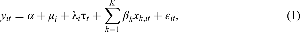
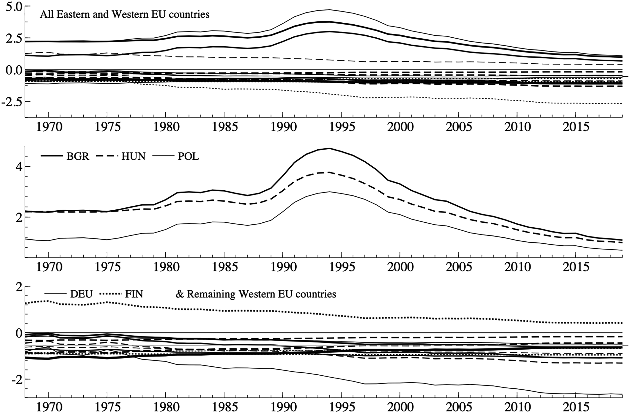
We present time series plots of the homicide rates for each of the 17 investigated countries (listed in the Appendix) from 1968 to 2019 in Figure 1. There are some countries with a few missing observations, but, as discussed in Section 3.2, our estimation methodology can handle such unbalanced panel data sets.

Figure 1.

Time series plots of the homicide rates per 100,000 inhabitants between 1968 and 2019. Top panel for all 17 EU countries, in-between panel for the top five countries (Eastern EU countries Bulgaria, Hungary and Poland plus Western EU countries Finland and Italy), and bottom panel for the remaining 12 Western EU countries. The full list of countries is given in the Appendix.

The top panel of Figure 1 depicts the data for all 17 countries and shows some noteworthy level differences. Three countries show homicide rates that are considerably higher than the other EU countries, namely Bulgaria, Finland and Hungary. In the early 1990s, homicide rates in Italy and Poland come close to these three countries. Therefore, the in-between panel of Figure 1 only plots these ‘top 5’ countries, whereas the bottom panel plots the homicide rates for the remaining 12 countries. We note that the top five countries are formed by all three Eastern EU countries in our sample (Bulgaria, Hungary and Poland) and two Western EU countries (Finland and Italy). Several authors attribute the higher number of homicides in Finland to alcohol consumption (Lehti and Sirén, 2020; Liem et al., 2013; Rossow, 2001) and the increase in number of homicides in Italy in 1992 to the mafia (Preti and Macciò, 2011; Vichi et al., 2020).

For the top five countries, the homicide rates fluctuate excessively from 1968 until the 1990s, with the homicide rate between one and three homicides per 100,000 inhabitants. Thereafter, the homicide rate first steeply increases to four to five homicides per 100,000 inhabitants (for Bulgaria the rate even doubles between 1987 and 1993), followed by a rapid decrease commencing between 1995 and 2000, which continues until the end of the sample period in 2019. In the final years of the sample period, all five countries are on their lowest point and show a rate of around one homicide per 100,000 inhabitants.

For the remaining twelve Western EU countries, the development in the homicide rate over time is more subtle (besides the initial peak for Germany): for these countries the rate increases slightly until 1990, after which it slightly decreases. The homicide rates of those Western EU countries in 2019 are on similar levels as those in 1968. For most countries, the homicide rate varies between one-half and just above one homicide per 100,000 inhabitants throughout the entire sample period.

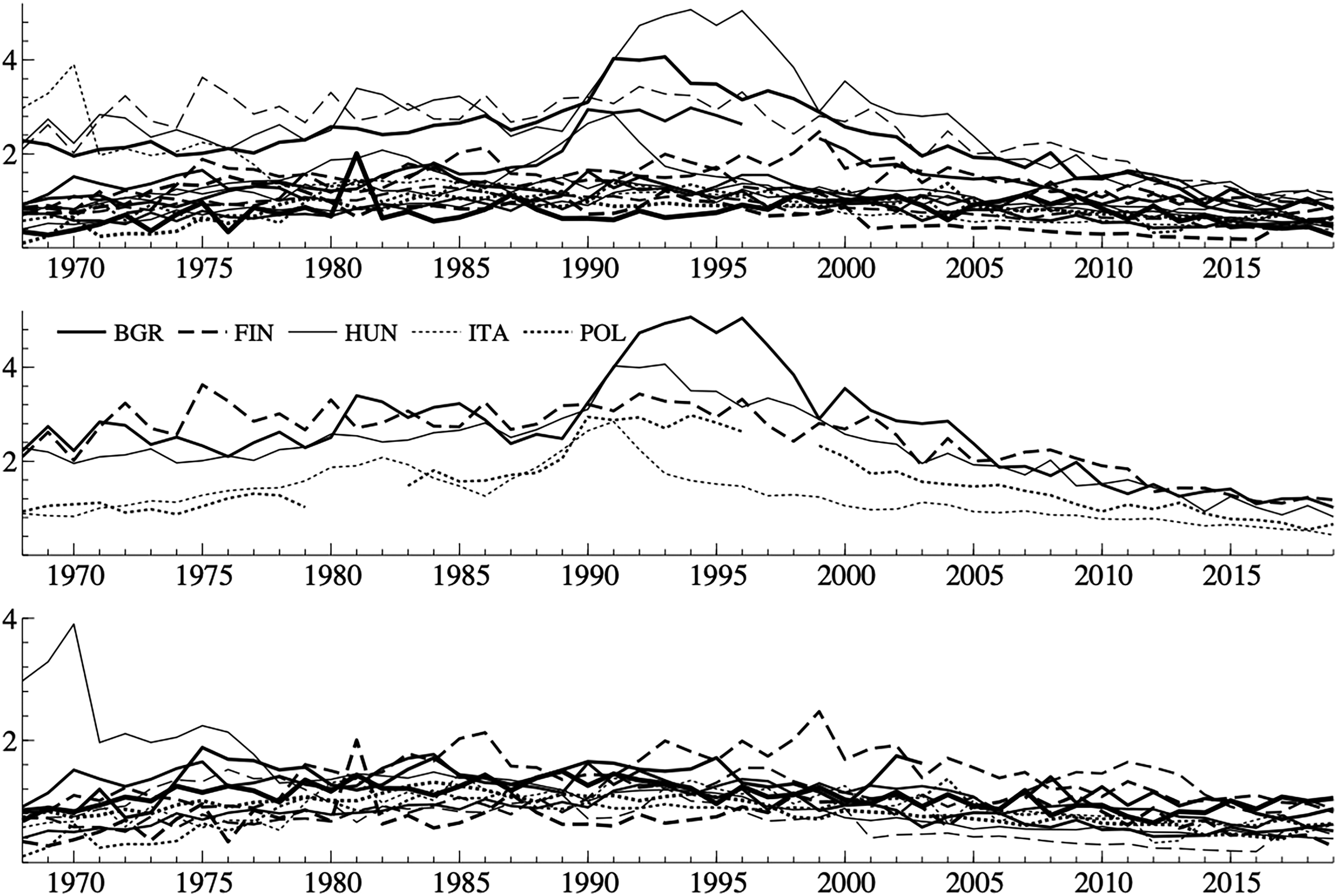
The time series plots of gross domestic product (GDP) growth rates and welfare growth for all 17 countries between 1968 and 2019 are provided in Figure 2. We clearly see that for both macroeconomic series, expansions are followed by contractions and vice versa. On the outset it might seem that the two are almost perfectly co-moving with each other, however, it is regularly not the case that as GDP increases/decreases that welfare also increases/decreases as, for example, is evidenced by the on-average 5.7 countries per year for which GDP increased while welfare decreased. In these cases, the signs of GDP growth rates and welfare growth do not align; it is this variation in the data that can be exploited for estimation purposes. Hence, this variation allows us to differentiate between the effects of macroeconomic activity (GDP growth rate) and macroeconomic performance (welfare growth).

Figure 2.

Time series plots of GDP growth rates (top panel) and welfare growth (bottom panel) for all 17 EU countries between 1968 and 2019. The full list of countries is given in the Appendix.

Finally, the young adult ratio (YAR) for all countries is presented in Figure 3. The top panel shows data for all 17 countries, while the in-between and bottom panels separate the Eastern and Western EU countries, respectively. Although the share of 25- to 34-year-olds in the total population remains fairly consistent across countries and over time, there is a notable difference between the regions around 1990. The YAR peaks for all three Eastern EU countries in the first half of the 1980s, then declines until the mid-1990s, after which it rises again. In contrast, the YAR remains relatively stable for the Western EU countries during this period. Thus, this population measure also highlights important regional and temporal differences.

Figure 3.

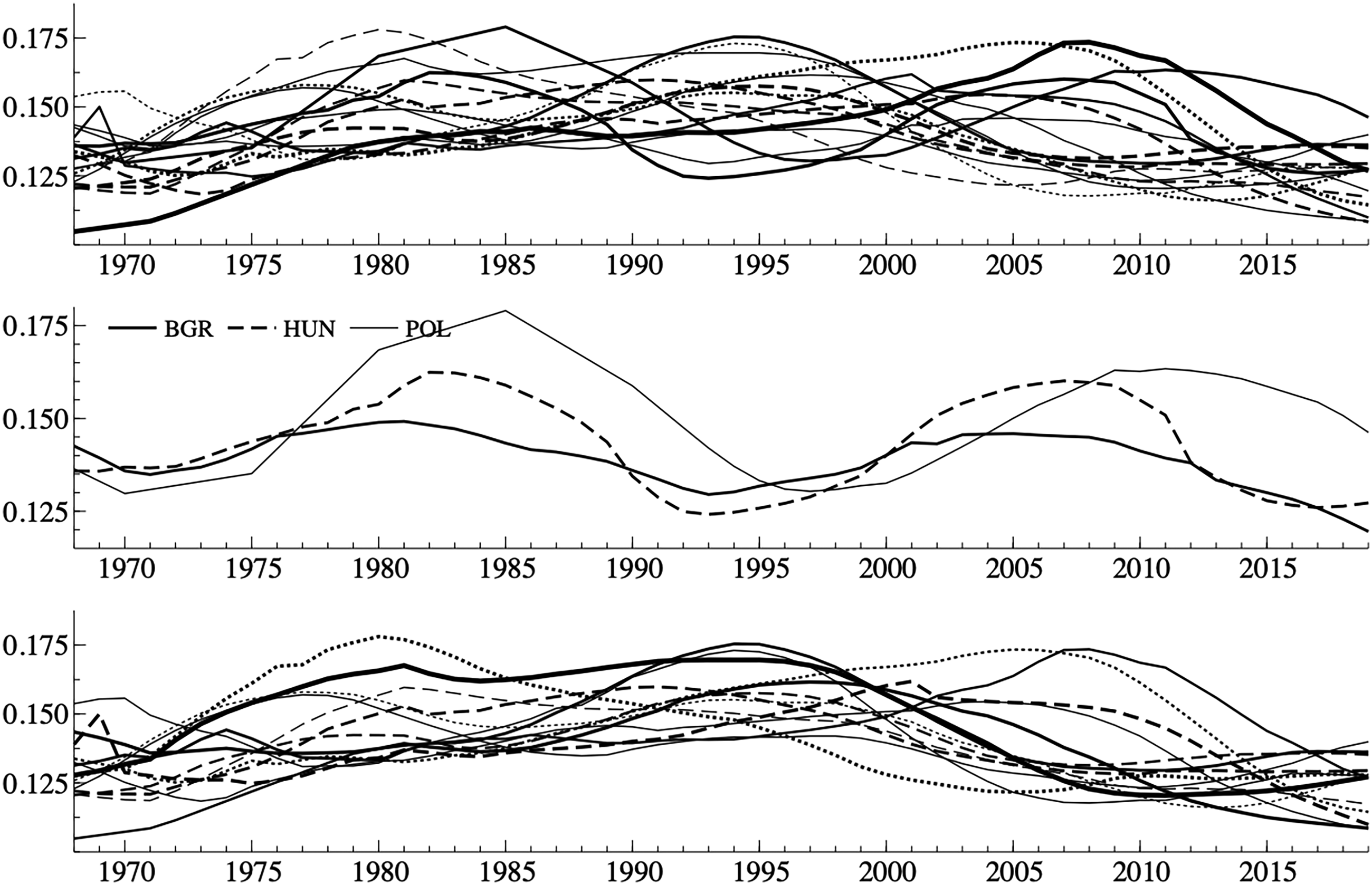
Time series plots of the YAR between 1968 and 2019. Top panel for all 17 EU countries, in-between panel for the Eastern EU countries (Bulgaria, Hungary and Poland), and bottom panel for the Western EU countries. The full list of countries is given in the Appendix.

Estimating the crime drop in EU countries

To estimate the underlying EU crime trend, we use the econometric model as outlined in Section 3.2. We first consider the model specification without macroeconomic and demographic explanatory variables. Figure 4 presents the estimated time-varying factors, where the solid line can be interpreted as the common EU crime trend underlying the homicide rate data. The dotted lines around the estimated crime trend indicate the 95% confidence interval and the crime trend is significantly varying over time. Moreover, the model is clearly able to capture the EU crime drop as the time-varying factor is increasing until the early 1990s, and it decreases directly after, to a lower level than in the 1970s.

Figure 4.

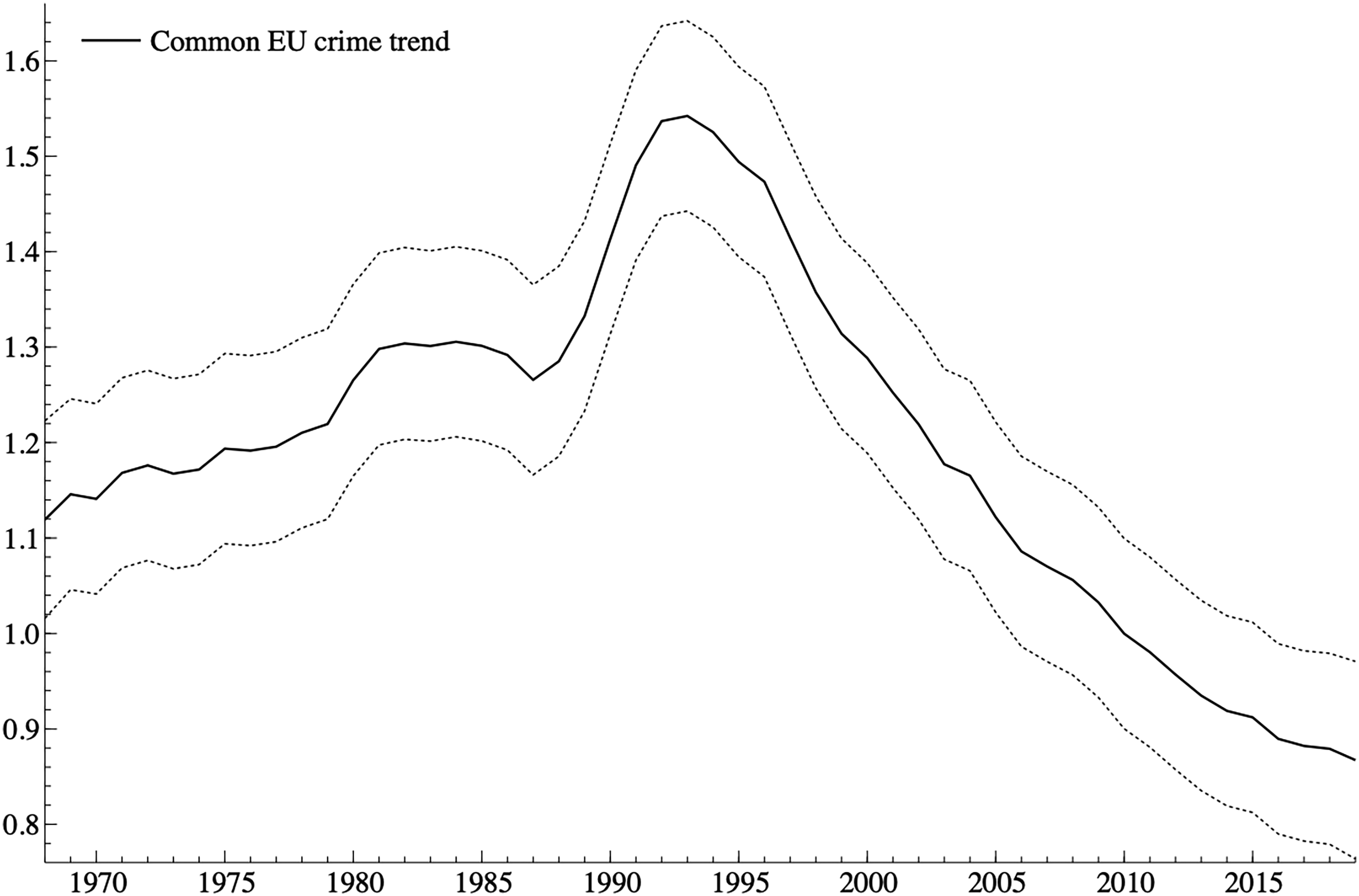
The estimated common EU crime trend (solid line), plotted with the 95% confidence interval (dotted lines).

We have also estimated to which extent each country experiences the common EU crime trend. The corresponding country-specific weights are visualized in Figure 5, where we have used Germany as the reference country with its weight fixed at unity. Bulgaria, Finland, Hungary, Italy and Poland (the ‘top 5’ countries of Figure 1) rely on the crime trend strongly, while the estimated weights of Greece and Ireland are very small. Furthermore, there is some moderate variation within the estimated weights of the other countries: countries like Denmark, France, UK, Netherlands and Portugal are closely aligned with Germany, while Austria and Belgium have somewhat larger weights, and Spain and Sweden have somewhat smaller weights. The main conclusion here is that most EU countries have been subject to the sizable crime drop as implied by the estimated common crime trend.

Figure 5.

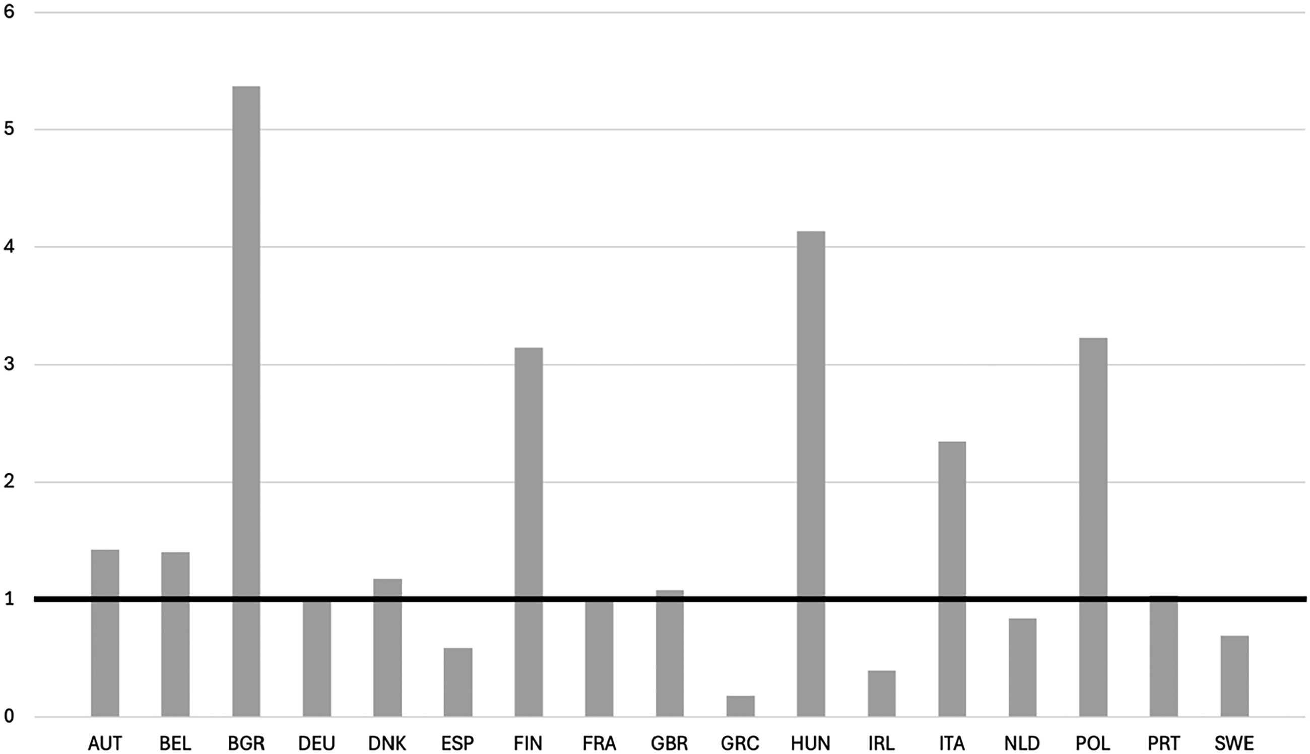
Estimated country-specific weights, indicating how much each country experienced the common EU crime trend of Figure 4. Germany is the reference country with its weight fixed at unity (solid line). The full list of countries is given in the Appendix.

Differences in the crime drop between western and eastern EU countries

The model can be extended with more time-varying factors to provide a better description of the dynamic properties of time series. In our model for the EU crime drop, we also have included a second crime trend that is exclusively associated with the Eastern EU countries Bulgaria, Hungary and Poland. In this way, we can analyze whether there is a ‘surplus factor’ for Eastern EU countries on top of the common EU crime trend. We have split the estimation results over two panels in Figure 6, which can be interpreted as follows. The top panel is the common crime trend as experienced by all EU countries, to a smaller or larger extent, depending on the estimated weights. The bottom panel represents the surplus factor as experienced by the Eastern EU countries only.

Figure 6.

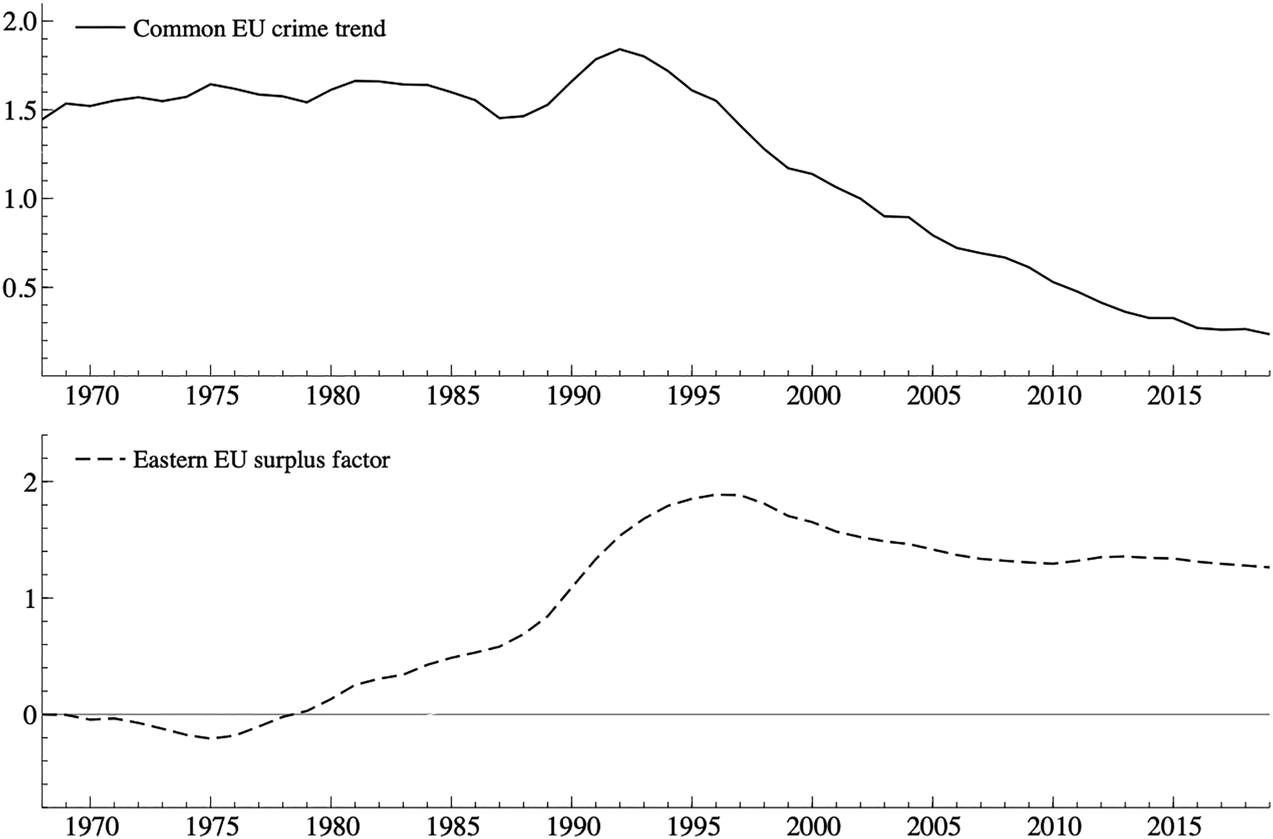
The estimated common EU crime trend as experienced by all EU countries (top panel) and the surplus factor for Eastern EU countries (bottom panel).

In the previous model specification, with a single time-varying factor, the estimated trend (Figure 4) shows an increase in the crime trend from 1968 to the early 1990s, followed by a notable decline. When we additionally allow for a second time-varying factor specific to Eastern EU countries, as in Figure 6, the increase from 1975 to the mid-1990s is attributed to the Eastern EU surplus factor (bottom panel), while the subsequent decline reflects the common EU crime trend (top panel). Western EU countries follow only a weighted version of the first common EU crime trend,⁷ suggesting a relatively stable crime pattern until the early 1990s, with a convincing drop thereafter. In contrast, Eastern EU countries follow a weighted average of both the common EU crime trend and the East EU surplus factor,⁸ resulting in an increasing crime trend before the 1990s and a smaller drop after.

Adding macroeconomic and demographic explanatory variables

The model with two time-varying factors for crime trends in Western and Eastern EU countries can be further extended with explanatory variables. We include two macroeconomic variables (GDP growth rates and welfare growth) and one demographic variable (the young adult ratio, YAR) in two different model specifications. In the first model specification, we allow the explanatory variables to have the same regression parameters for all EU countries, that is a fully pooled regression. In the second model specification, we have different parameters for Western and Eastern EU countries, that is a partially pooled regression. Hence, the two regions of countries can experience different effects. We present the estimation results in Table 1.

Table 1.

Parameter estimation results for a model with common EU crime trend and Eastern EU surplus factor. The explanatory variables are in columns (from left to right: GDP growth rate, welfare growth and YAR). The first line ‘EU overall’, shows the results of a model where all EU countries experience the same effect (fully pooled). The second line ‘Western EU’ and third line ‘Eastern EU’ shows the results of a model where Western and Eastern EU countries, respectively, are allowed to experience different effects (partially pooled). The estimated parameters are given, with standard errors in parentheses, and where * denotes a 10% significance level, ** 5%, and *** 1%.

	GDP growth rate	Welfare growth	YAR
EU overall	−0.481 (0.333)	−0.876 (0.356)**	10.88 (0.72)***
Western EU	−0.003 (0.368)	−1.444 (0.396)***	11.80 (0.72)***
Eastern EU	−2.251 (0.739)***	1.313 (0.781)*	0.42 (3.10)

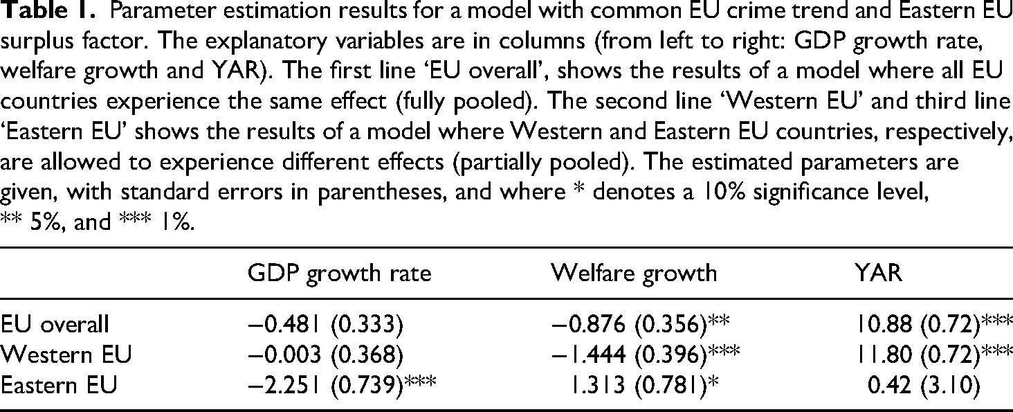
We find that overall, for all EU countries, the macroeconomic effects for increases in activity and performance are negative. In particular, the estimate for GDP growth rate is −0.481 but only approaches significance at the 10%-level, while the estimate for welfare growth is −0.876 and is significant at the 5%-level. It implies that better economic conditions are associated with a decrease in homicide rates. The YAR has a strong positive effect that is significant at the 1%-level. It implies that a higher share of 25- to 34-year-olds in the population is strongly associated with an increase homicide rates.

When we compare the overall effects to regional effects, we find remarkable differences. GDP growth rates turn out to have only relevance for the Eastern EU countries: the estimated parameter of −2.251 is highly significant at the 1%-level, while the corresponding estimate for Western EU countries is not significant. The opposite conclusion can be made for welfare growth, where the overall results turn out to be mostly driven by Western EU countries: the estimated parameter of −1.444 for Western EU is highly significant at the 1%-level. The corresponding estimate for Eastern EU has an estimate of 1.313 but is only significant at the 10%-level, in a positive direction. Further, the effect of the YAR is clearly driven by Western EU countries, with a positive estimate of 11.80, highly significant at the 1%-level, but no significant effect for Eastern EU countries. These results imply that more macroeconomic activity (increasing GDP growth rates) is associated with a decrease in homicide in Eastern EU countries, better macroeconomic performance (increasing welfare growth) is associated with a decrease in homicide in Western EU countries and a weak increase in Eastern EU countries, and a larger share of 25- to 34-year-olds in the total population is associated with an increase in homicide in Western EU countries.

When we include only the two macroeconomic explanatory variables in the model specification, the estimated crime trends remain broadly unchanged compared to those shown in Figure 6. They indicate that the crime drop phenomenon clearly persists in the data, even after controlling for macroeconomic circumstances. This suggests that, although the economic variables have significant effects, they alone do not fully account for the observed crime drop in EU homicide rates during the period under investigation. No additional impact on the crime trend around the start of the European debt crisis in 2009 is apparent, which further indicates that short-term macroeconomic fluctuations are not strongly associated with the EU crime drop. Hence, there may be other factors that drive the EU crime drop more strongly.

When the demographic explanatory variable is included in the model, as the only one or together with the macroeconomic explanatory variables, the estimated crime trends change noticeably from those depicted in Figure 6. Since also the country-specific fixed effects and country-specific weights change considerably compared to those discussed for previous model specifications (Figure 5 and footnotes 7 and 8), we present the results in a disaggregated form. Figure 7 displays the estimated overall country-specific time-varying trends after controlling for both macroeconomic and demographic explanatory variables with regional effects.⁹ The top panel shows the estimated trends for all 17 countries, while the in-between and bottom panels present the trends for Eastern and Western EU countries, respectively.

Figure 7.

Plots of the overall country-specific time-varying trends between 1968 and 2019 after controlling for the macroeconomic and demographic explanatory variables with regional effects, in a model with common EU crime trend and Eastern EU surplus factor. Top panel for all 17 EU countries, in-between panel for the Eastern EU countries (Bulgaria, Hungary and Poland), and bottom panel for the Western EU countries. The full list of countries is given in the Appendix.

We find that the overall country-specific time-varying trends for Western EU countries are small and noticeably stable over time. Most Western EU countries follow a highly similar pattern, with only Finland displaying a somewhat higher trend and Germany a somewhat lower trend. Since these stable trends emerge only after controlling for the YAR, this population measure appears to substantially explain the crime trend and drop in Western EU countries. In contrast, Eastern EU countries continue to exhibit an increasing trend until the early 1990s followed by a subsequent decline, consistent with the insignificant YAR parameter estimate reported in Table 1, and confirming that the YAR does not contribute much in explaining the crime drop in Eastern EU countries.

Evaluating model properties

Finally, we assess the overall performance of our econometric model through a goodness-of-fit measure. Table 2 presents the log likelihood values of all model specification variations considered in this study. A higher log likelihood value indicates a better fit of the model to the data, here represented by values closer to zero. Model (1) is the model with only a common EU crime trend (results in Section 4.2). Model (2) adds flexibility by introducing an Eastern EU surplus factor, yielding separate Western and Eastern EU crime trends (Section 4.3). Model (3) builds on model (2) by including the explanatory variables (GDP growth rate, welfare growth and the YAR), with same effects for all EU countries (Section 4.4), and model (4) further enhances flexibility by allowing for different effects for Western and Eastern EU countries (also Section 4.4).

Table 2.

Model fit of all considered variations of our model. The column headers refer to Model 1 from Section 4.2: common EU crime trend, Model 2 from Section 4.3: Western and Eastern EU crime trends, Model 3 from Section 4.4: Western and Eastern EU crime trends plus common macroeconomic and demographic effects, and Model 4 from Section 4.4: Western and Eastern EU crime trends plus Western and Eastern EU macroeconomic and demographic effects. A higher log likelihood value indicates a better fit of the model to the data.

Model	(1)	(2)	(3)	(4)
Log likelihood value	−300.94	−227.92	−168.46	−154.57

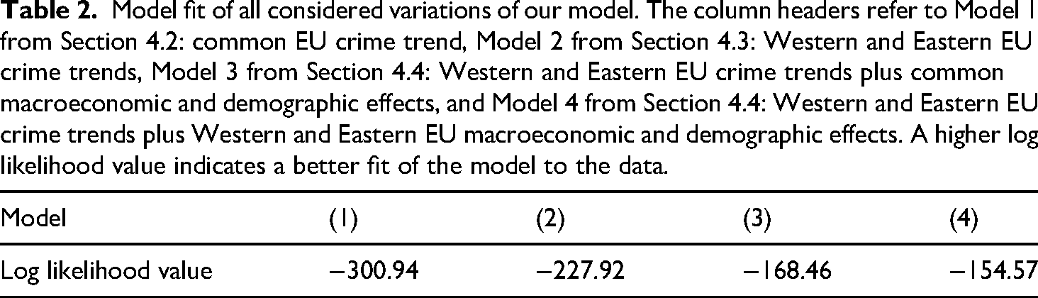
Model (1) closely resembles a two-way fixed effects model. The differences are that we have a stochastically time-varying factor rather than time fixed effects and, most importantly, we allow that each country can experience its own weighted version of the common EU crime trend, rather than all countries identically experiencing the crime trend. However, if we fix the weights to unity, instead of estimating them, the model approximates a two-way fixed effects model. The log likelihood value would then be −509.01, which is substantially lower than the log likelihood value of −300.94 for model (1). This shows the benefit of allowing for country-specific weights in our model compared to the unit weights used in two-way fixed effects models.¹⁰

A notable improvement in log likelihood values is from −300.94 for model (1) to −227.92 for model (2). This demonstrates the value of differentiating between Western and Eastern EU crime trends. Further improvements become apparent when we include macroeconomic and demographic explanatory variables, as model (3) shows an increased log likelihood value of −168.46. The log likelihood value for model (4) increases further to −154.57, showing that it is beneficial to allow the macroeconomic and demographic effects to differ between Western and Eastern EU countries.

Overall, each extension of our model improves the fit to the data. Therefore, model (4) is the preferred model in our study, from which we conclude that it is beneficial to allow for country-specific weights for the common EU crime trend, differentiating between Western and Eastern EU countries, and including macroeconomic and demographic explanatory variables with distinct regional effects.

Conclusions

In this paper, we developed a panel data model with stochastically time-varying factors to analyze country-level crime trends in greater detail, focusing on the crime drop in EU countries. Our objectives were to showcase the model's capabilities, investigate whether a drop in homicide rates occurred, examine how closely individual countries followed the common trend, explore regional differences in timing and magnitude, and evaluate effects of explanatory variables, using macroeconomic and demographic indicators.

Main findings and achievements

Our first and main aim of exploring the newly developed modeling approach revealed that the proposed model served its purposes. The model was able to estimate a common crime trend for 17 EU countries, to analyze how country-level trends varied with regard to this general trend, to estimate the effects of explanatory variables, and to detect different effects across EU regions. Our evaluation of model fit for subsequently elaborated models showed that adding new elements in the model resulted in better fits. It also illustrated that our modeling approach provides advantages over previous models to analyze crime trends, for example two-way fixed models that were used by Rosenfeld and Messner (2012).

The second aim of this paper was to establish whether there indeed has been a crime drop in homicide in the EU, the focus of our study. Our analysis showed that such a general drop indeed exists and started in the early 1990s.

Regarding our third goal concerning regional differences in the crime trend, we showed that all countries experienced their own weighted versions of the crime trend. These findings add to the debate opened by Aebi and Linde (2010), who questioned the presence of an overall European crime drop. Our findings show that the crime drop is present in Eastern EU countries, but less pronounced than in Western EU countries. This means that earlier presented results for Western EU countries are not automatically generalizable to the EU or Europe (e.g., Aebi and Linde, 2010, 2012, 2014).

Our fourth goal was to evaluate the possibilities of the model to estimate potential explanations for the trend in homicide, while allowing for regional differences. Our results showed that we could indeed establish effects of macroeconomic and demographic indicators.

In line with previous findings (e.g., Rosenfeld and Levin, 2016; Rosenfeld and Messner, 2012; Van Dijk et al., 2021), the overall effects of macroeconomic conditions were relatively modest. Broadly speaking, we find that macroeconomic circumstances are inversely related to crime, supporting sociological and economic theories that suggest prosperity leads to better living conditions, reduced poverty, stronger institutional legitimacy and the opportunity to invest in policing and prevention (LaFree, 2018; Messner et al., 2001; Tonry, 2014). Interestingly, the estimated effects of the two macroeconomic indicators differ between EU regions, both in magnitude and, in one case, in direction. In Eastern EU countries, macroeconomic activity (GDP growth rate) was associated with a decrease in homicide, whereas in Western EU countries only macroeconomic performance (welfare growth) showed a negative effect, and it may have been positive in Eastern EU countries. Societal transformations in Eastern EU around the dissolution of the Soviet Union and the fall of the Berlin Wall may have shaped how macroeconomic changes affected crime through increased inequality and relative deprivation (Merton, 1938; Messner et al., 2001). Economic activity may have been more important for institutional legitimacy and economic opportunities for relatively deprived parts of the population than in Western EU. Growth in welfare may also have increased feelings of relative deprivation following the communist period in Eastern EU.

The overall effect of the young adult population on homicide trends was larger than that of macroeconomic changes, consistent with earlier research linking age structure to homicide trends. Santos et al. (2019) show that the proportion of young people aged 15–30 is an important predictor over longer periods. The Global Study on Homicide (UNODC, 2023) similarly highlights demographic changes as key factors, although their effects vary across countries. Consistent with this, we find pronounced regional differences: the effect of age composition is strong in Western EU countries but negligible in Eastern EU countries. In Western EU, it explains a substantial part of the homicide drop. Possible explanations include differences in the peak age for homicide or other region-specific drivers that outweigh the influence of age composition in Eastern EU.

In sum, the EU crime drop reflects multiple global and region-specific mechanisms. In Eastern EU, the decline coincides with historical transitions following the dissolution of the Soviet Union and the fall of the Berlin Wall, likely shaping economic opportunities, social institutions, and (feelings of) relative deprivation, and in turn influencing crime patterns, consistent with classic and general strain theory (Agnew, 1992; Merton, 1938) and routine activity theory (Cohen and Felson, 1979). In Western EU, where institutions and social support were more stable, improvements in welfare may have reduced homicide through improved social stability and reduced strain, consistent with strain theories and institutional anomie theory (Messner and Rosenfeld, 1997). Demographic composition, captured by the share of young adults, played a substantial role in Western EU but not Eastern EU, suggesting that age structure interacts with historical and institutional conditions in shaping crime trends. Cultural change and economic uncertainty may have differentially affected crime rates across age groups, flattening the age-crime distribution (Steffensmeier et al., 2025). Taken together, these observations indicate that macroeconomic and demographic factors operated alongside broader social, institutional, and historical influences. Strategies to reduce crime could benefit from regionally tailored interventions, addressing economic opportunities and inequality in Eastern EU and supporting social cohesion and institutional capacity in Western EU.

Limitations and suggestions for future research

The main limitation of the current research is that it is based solely on homicide rates. Our findings may not generalize to other common crime types, such as property or drug crimes (Aebi and Linde, 2010, 2011, 2012, 2014; Killias and Aebi, 2000). Future research can focus on other crime types but can also examine disaggregated homicide subtypes and explain these trends (Suonpää et al., 2024). Moreover, homicide data itself is not perfectly reliable across sources, as differences between the WHO Mortality Database and the UNODC Homicide Data have recently been documented by Santos and Testa (2024). Data availability further limits external validity, as generalization to Eastern EU or Europe is based on only three countries, and prevents us from assessing the years after 2019, including the impact of the Covid-19 pandemic from 2020 onward.

Secondly, several potentially relevant explanatory variables were not included in the model. For example, our current welfare measure reflects economic efficiency rather than direct government spending, and future work could use social welfare expenditures as a more direct indicator of decommodification, aligning with institutional anomie theory (Pridemore and Kim, 2006). Moreover, as Rosenfeld and Levin (2016) noted, the absence of inflation during the Great Recession helped explain stable crime rates in the US, suggesting inflation could be a useful addition if such data become available. Other macro-level variables, including those facilitating or inhibiting crime or related to the functioning of the criminal justice system, could also be incorporated (Spelman, 2022).

Finally, we did not make any causal claims regarding macroeconomic or demographic variables or the mechanisms behind homicide rates. Future research could explore causal effects more directly. Differences in policies or unexpected events across countries could be exploited to estimate causal impacts, and Harvey and Thiele (2021) showed that this is feasible for dynamic models like ours. However, sufficient data from before 1990 remain scarce, not only for different types of crime but also for other macro-level variables.

Our study is, to our knowledge, the first to model the crime drop as a stochastically time-varying factor, incorporating country-specific weights on crime trends and the inclusion of explanatory variables, with different regional effects. Such an extended econometric specification would be very cumbersome, if not impossible, in the setting of more traditional models, such as the two-way fixed effects model. Given the availability of suited panel data, our approach provides a new opportunity to study the way in which crime develops over time and in different jurisdictions, and to test theoretically derived hypotheses on how crime developments originate.

Footnotes

ORCID iDs

Ilka van de Werve

Siem Jan Koopman

Ethical considerations

There are no human participants in this article and informed consent is not required.

Funding

The author(s) received no financial support for the research, authorship, and/or publication of this article.

Declaration of conflicting interests

The author(s) declared no potential conflicts of interest with respect to the research, authorship and/or publication of this article.

Data availability

The datasets generated during and/or analyzed during the current study are available from the corresponding author on reasonable request.

Notes

Appendix List of countries and country codes

The binary classification for Western and Eastern EU countries is based on the Regional Groups of Member States of the United Nations, where Bulgaria, Hungary and Poland are grouped as Eastern EU and marked with an asterisk in the list above.

References

Aebi

Linde

(2010) Is there a crime drop in Western Europe? European Journal on Criminal Policy and Research 16: 251–277.

Aebi

Linde

(2011) Regional variation in Europe between homicide and other forms of external death and criminal offences. In: Handbook of European Homicide Research: Patterns, Explanations, and Country Studies. New York: Springer, 71–94.

Aebi

Linde

(2012) Crime trends in Western Europe according to official statistics from 1990 to 2007. The International Crime Drop: New Directions in Research. Springer: 37–75.

Aebi

Linde

(2014) The persistence of lifestyles: Rates and correlates of homicide in Western Europe from 1960 to 2010. European Journal of Criminology 11(5): 552–577.

Aebi

Linde

(2016) Long-term trends in crime. In: The Oxford Handbook of the History of Crime and Criminal Justice: 57–87.

Agnew

(1992) Foundation for a general strain theory of crime and delinquency. Criminology; An Interdisciplinary Journal 30(1): 47–88.

Berg

Baumer

Rosenfeld

, et al. (2016) Dissecting the prevalence and incidence of offending during the crime drop of the 1990s. Journal of Quantitative Criminology 32: 377–396.

Blumstein

(2017) Some trends in homicide and its age-crime curves. The Handbook of Homicide: 44–53.

Blumstein

Rosenfeld

(1997) Explaining recent trends in US homicide rates. Journal of Criminal Law & Criminology 88: 1175.

10.

Blumstein

Wallman

(2006) The crime drop and beyond. Annual Review of Law and Social Science 2(1): 125–146.

11.

Cohen

Felson

(1979) Social change and crime rate trends: A routine activity approach. American Sociological Review: 588–608.

12.

Daly

Wilson

Vasdev

(2001) Income inequality and homicide rates in Canada and the United States. Canadian Journal of Criminology 43(2): 219–236.

13.

Doornik

(2021) Object-Oriented Matrix Programming using Ox, 9th ed. London: Timberlake Consultants Press.

14.

Durbin

Koopman

(2012) Time Series Analysis by State Space Methods. Oxford: OUP Oxford.

15.

Eisner

(2003) Long-term historical trends in violent crime. Crime and Justice 30: 83–142.

16.

Farrell

Birks

(2018) Did cybercrime cause the crime drop? Crime Science 7(1): 8.

17.

Farrell

Laycock

Tilley

(2015) Debuts and legacies: The crime drop and the role of adolescence-limited and persistent offending. Crime Science 4(1): 1–10.

18.

Farrell

Tilley

Tseloni

, et al. (2010) Explaining and sustaining the crime drop: Clarifying the role of opportunity-related theories. Crime Prevention and Community Safety 12: 24–41.

19.

Farrell

Tilley

Tseloni

(2014) Why the crime drop? Crime and Justice 43(1): 421–490.

20.

Feenstra

Inklaar

Timmer

(2015) The next generation of the Penn World Table. American Economic Review 105(10): 3150–3182.

21.

Harvey

Thiele

(2021) Cointegration and control: Assessing the impact of events using time series data. Journal of Applied Econometrics 36(1): 71–85.

22.

Heitmeyer

Haupt

H-G

Kirschner

, et al. (2011) Control of violence. In: Historical and International Perspectives on Violence in Modern Societies. New York: Springer.

23.

Hirschi

Gottfredson

(1983) Age and the explanation of crime. American Journal of Sociology 89(3): 552–584.

24.

Killias

Aebi

(2000) Crime trends in Europe from 1990 to 1996: How Europe illustrates the limits of the American experience. European Journal on Criminal Policy and Research 8: 43–63.

25.

Koopman

Shephard

Doornik

(1999) Statistical algorithms for models in state space using SsfPack 2.2. The Econometrics Journal 2(1): 107–160.

26.

LaFree

(2018) Losing Legitimacy: Street Crime and the Decline of Social Institutions in America. New York: Routledge.

27.

LaFree

Curtis

McDowall

(2015) How effective are our ‘better angels’? Assessing country-level declines in homicide since 1950. European Journal of Criminology 12(4): 482–504.

28.

La Free

Drass

(2002) Counting crime booms among nations: Evidence for homicide victimization rates, 1956 to 1998. Criminology; An Interdisciplinary Journal 40(4): 769–800.

29.

LaFree

Tseloni

(2006) Democracy and crime: A multilevel analysis of homicide trends in forty-four countries, 1950–2000. The Annals of the American Academy of Political and Social Science 605(1): 25–49.

30.

Lappi-Seppälä

Lehti

(2014) Cross-comparative perspectives on global homicide trends. Crime and Justice 43(1): 135–230.

31.

Lehti

Sirén

(2020) The impact of alcohol consumption on homicide: A time-series analysis of three nordic countries. European Journal of Criminology 17(3): 352–369.

32.

Liem

Ganpat

Granath

, et al. (2013) Homicide in Finland, The Netherlands, and Sweden: First findings from the European homicide monitor. Homicide Studies 17(1): 75–95.

33.

Liem

Pridemore

(2012) Handbook of European Homicide Research: Patterns, Explanations, and Country Studies. New York: Springer.

34.

Merton

(1938) Social structure and anomie. American Sociological Review 3(5): 672–682.

35.

Messner

Raffalovich

McMillan

(2001) Economic deprivation and changes in homicide arrest rates for white and black youths, 1967–1998: A national time-series analysis. Criminology; An Interdisciplinary Journal 39(3): 591–614.

36.

Messner

Rosenfeld

(1997) Political restraint of the market and levels of criminal homicide: A cross-national application of institutional-anomie theory *. Social Forces 75(4): 1393–1416.

37.

Mitra

Abedin

Sen

(2023) Does an ageing population affect crime rates in the United States? Social Indicators Research 170(3): 825–845.

38.

Moffitt

Caspi

(2005) Life-course persistent and adolescence-limited antisocial males: Longitudinal followup to adulthood. Developmental Psychobiology of Aggression 12: 161–186.

39.

O’Brien

(2019) Homicide arrest rate trends in the United States: The contributions of periods and cohorts (1965–2015). Journal of Quantitative Criminology 35: 211–236.

40.

O'Brien

Stockard

(2002) Variations in age-specific homicide death rates: A cohort explanation for changes in the age distribution of homicide deaths. Social Science Research 31(1): 124–150.

41.

Parker

Mancik

Stansfield

(2017) American Crime drops: Investigating the breaks, dips and drops in temporal homicide. Social Science Research 64: 154–170.

42.

Preti

Macciò

(2011) Homicide in Italy. In: Handbook of European Homicide Research: Patterns, Explanations, and Country Studies. New York: Springer, 373–389.

43.

Pridemore

Kim

S-W

(2006) Democratization and political change as threats to collective sentiments: Testing durkheim in Russia. The Annals of the American Academy of Political and Social Science 605(1): 82–103.

44.

Rogers

Pridemore

(2018) Do national homicide rates follow supranational trends? Journal of Research in Crime and Delinquency 55(6): 691–727.

45.

Rosenfeld

Levin

(2016) Acquisitive crime and inflation in the United States: 1960–2012. Journal of Quantitative Criminology 32: 427–447.

46.

Rosenfeld

Messner

(2012) The crime drop in comparative perspective: The impact of the economy and imprisonment on American and European burglary rates. In: van Dijk

Tseloni

Farrell

(eds) The International Crime Drop: New Directions in Research. London: Palgrave Macmillan UK, 200–228.

47.

Rosenfeld

Weisburd

(2016) Explaining recent crime trends: Introduction to the special issue. Springer. 329–334.

48.

Rossow

(2001) Alcohol and homicide: A cross-cultural comparison of the relationship in 14 European countries. Addiction 96(1s1): 77–92.

49.

Sampson

Laub

(1995) Crime in the Making: Pathways and Turning Points Through Life. Cambridge: Harvard University Press.

50.

Santos

Fairchild

(2021) Age, period and cohort differences between the homicide trends of Canada and the United States. The British Journal of Criminology 61(2): 389–413.

51.

Santos

Testa

(2024) Global trends in homicide: A comparison between the UNODC homicide data and the WHO mortality database. In: Routledge Handbook of Homicide Studies. New York: Routledge, 7–40.

52.

Santos

Testa

Porter

, et al. (2019) The contribution of age structure to the international homicide decline. PLoS One 14(10): e0222996.

53.

Spelman

(2022) How cohorts changed crime rates, 1980–2016. Journal of Quantitative Criminology 38(3): 637–671.

54.

Steffensmeier

Slepicka

Schwartz

(2025) International and historical variation in the age–crime curve. Annual Review of Criminology 8(Volume 8, 2025): 239–268.

55.

Steffensmeier

Harer

(1987) Is the crime rate really falling? An ‘aging’ US population and its impact on the nation's crime rate, 1980–1984. Journal of Research in Crime and Delinquency 24(1): 23–48.

56.

Suonpää

Kivivuori

Aarten

, et al. (2024) Homicide drop in seven European countries: General or specific across countries and crime types? European Journal of Criminology 21(1): 3–30.

57.

Tonry

(2014) Why crime rates are falling throughout the western world. Crime and Justice 43(1): 1–63.

58.

Tseloni

Mailley

Farrell

, et al. (2010) Exploring the international decline in crime rates. European Journal of Criminology 7(5): 375–394.

59.

UNODC (2023) Global Study on Homicide 2023. New York: United Nations.

60.

Van Dijk

Nieuwbeerta

Joudo Larsen

(2021) Global crime patterns: An analysis of survey data from 166 countries around the world, 2006–2019. Journal of Quantitative Criminology: 1–36.

61.

Van Dijk

Tseloni

Farrell

(2012) The international crime drop: New directions in research.

62.

Vichi

Ghirini

Roma

, et al. (2020) Trends and patterns in homicides in Italy: A 34-year descriptive study. Forensic Science International 307: 110141.

63.

Weiss

Santos

Testa

, et al. (2016) The 1990s homicide decline: A western world or international phenomenon? A research note. Homicide Studies 20(4): 321–334.

64.

Wellford

(1973) Age composition and the increase in recorded crime. Criminology; An Interdisciplinary Journal 11: 61.

65.

Westfelt

Estrada

(2012) International crime trends: Sources of comparative crime data and post-war trends in Western Europe. Transnational and Comparative Criminology. Routledge-Cavendish: 19–48.

66.

Zimring

(2006) The Great American Crime Decline. New York: Oxford University Press.

Exploring the crime drop in European Union homicide rates using econometric modeling

Abstract

Keywords

Introduction

Previous studies

Describing crime trends

Explaining crime trends

Modeling crime trends

Data and methodology

Data

The proposed model

Results

Descriptive findings

Estimating the crime drop in EU countries

Differences in the crime drop between western and eastern EU countries

Adding macroeconomic and demographic explanatory variables

Evaluating model properties

Conclusions

Main findings and achievements

Limitations and suggestions for future research

Footnotes

ORCID iDs

Ethical considerations

Funding

Declaration of conflicting interests

Data availability

Notes

Appendix List of countries and country codes

References