Performance of melanopsin-based spatial brightness metrics

Abstract

Traditional photometric measures, such as illuminance and luminance, often fail to accurately estimate spatial brightness. Recent studies suggest that melanopsin-containing intrinsically photosensitive retinal ganglion cells contribute to brightness in addition to cone cells, and new metrics have been developed to predict cone and melanopsin-driven brightness. This study evaluates the performance of three melanopsin-based spatial brightness metrics through two psychophysical experiments. A total of 39 pairs of lighting conditions were generated representing two nominal correlated colour temperatures (CCTs; 2700 K and 4700 K) and three vertical illuminances (40 lx, 75 lx and 120 lx) in experiment 1, and three nominal CCTs (2700 K, 4000 K and 6000 K) and three vertical illuminances (50 lx, 100 lx and 300 lx) in experiment 2. Results from both experiments indicate that melanopsin-based metrics exhibit limited predictive accuracy for spatial brightness. These results underscore the complexity of spatial brightness and highlight the limitations of current melanopsin-centric approaches. Future research should explore a wider range of illuminance levels and the role of spatial light distribution.

1. Introduction

Accurate measurement and standardisation of the perception of light have been a scientific challenge for centuries. ¹ The current photometric system provides reliable, yet imperfect measures of light to quantify the perceptual responses to optical radiation. Brightness, arguably the most important perceptual response to light, is often mistakenly associated with photometric measures (e.g. luminance, illuminance) despite their well-documented limitations.^2,3 While brightness is a perceptual construct, luminance and illuminance are physical measures of visible radiation. In addition to the criticism of the limitations of illuminance, the basis of photometric measures, the International Commission on Illumination (CIE) photopic luminous efficiency function (aka 2° standard observer), ⁴ has also been criticised for its limitations, such as the small field of view (FOV), ⁵ and alternatives have been proposed, including the CIE physiological axes. ⁶ Despite the significant differences between the standard and alternative functions,^7–9 the 2° standard observer is still used today to calculate photometric measures.

Meanwhile, spatial brightness, ‘attribute of a visual perception according to which a luminous environment appears to contain more or less light’, ¹⁰ has gained attention in lighting research.^11–18 It is indisputable that increased light levels leads to an increase in spatial brightness, albeit non-linearly – an effect known as the Stevens’ power law ² or Weber–Fechner law. ¹⁹ On the other hand, a secondary effect of spectral power distribution (SPD) on spatial brightness has been well-documented without a clear predictive metric. ²⁰ While some studies associate higher correlated colour temperature (CCT; T_cp) with increased spatial brightness,^12,21,22 others found no statistical impact of CCT on spatial brightness when the stimuli were controlled for colour fidelity and gamut.^23,24 Interestingly, a couple of studies showed that colour gamut can also contribute to spatial brightness, where increased gamut was linked with increased spatial brightness,^25,26 although one of these studies ²⁵ did not control CCT. Overall, the research literature indicate a potential impact of SPD on spatial brightness, but the modelling of this effect has been elusive so far.^20,27

Recently, the discovery of melanopsin photoreceptors in intrinsically photosensitive retinal ganglion cells (ipRGCs) and their role in visual and non-visual mechanisms led brightness studies into a new direction. Results from several studies suggest that ipRGC-influenced light responses ²⁸ is a key part of visual mechanisms, such as brightness.^24,29–31 On the other hand, studies controlling both chromatic and melanopsin contents suggest that melanopsin’s contribution to spatial brightness can be secondary to the chromatic contribution.^32,33 The unclear role of melanopsin in spatial brightness has not prevented researchers from developing spatial brightness models to predict the effects of melanopsin.^31,34,35

Rea et al. developed a scene brightness metric for outdoor lighting by adding a weighted S-cone spectral sensitivity s_SC $\left(\lambda \right)$ contribution to the CIE photopic luminous efficiency function V( $\lambda$ ). ³⁶ Based on this earlier study, they further developed the scene brightness spectral sensitivity function $B_v\left(\lambda \right)$ for indoor spaces using Equation (1)

$$B_v\left(\lambda \right)=V\left(\lambda \right)+(0.264\ln \left(E_v\right)+1.093)s_{\mathrm{sc}}\left(\lambda \right)+0.5s_{\mathrm{mel}}(\lambda )$$

(1)

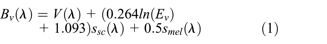
where s_mel( $\lambda$ ) is the ipRGC spectral sensitivity, ³⁷ and E_v is the vertical illuminance at the eye. ³⁴ The weighting function for the $s_{\mathrm{sc}}\left(\lambda \right)$ contribution is determined by the vertical illuminance at the observer’s eye position, and the constants in the equation were derived from a psychophysical experiment that utilised two horizontal illuminances (100 lx and 350 lx), two wall reflectances (0.2 and 0.7) and two CCTs (2700 K and 5400 K). The experimental apparatus was a booth of dimensions 0.56 m × 0.56 m × 0.56 m, having achromatic interior surfaces, with doll furniture simulating a living room and subtended a 34° FOV. Twelve participants used a magnitude estimation method to make subjective brightness judgements after 5 s. In this indoor scene brightness model, parameter $B$ is calculated using Equation (2)

$$B=\int P(\lambda )B_v\left(\lambda \right)\mathrm{d}\lambda$$

(2)

where $P(\lambda )$ is the SPD of the light source (spectral irradiance) at the eye level.

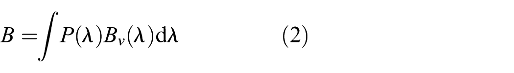
Somewhat similarly, Yamakawa et al. ³¹ formulated a metric (R) to model brightness at the cornea as a function of melanopsin using Equation (3)

$$R=4.84·{10}^{-3}·{\left(M\pi {\left(\frac{d}{2}\right)}^2\right)}^{1.1}+2.31·{\left(L\pi {\left(\frac{d}{2}\right)}^2\right)}^{0.48}$$

(3)

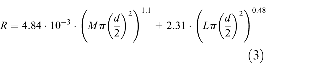
where d is the pupil diameter, M is the melanopsin stimulation and L is luminance at the cornea. In their model, pupil diameter ( $d$ ) and melanopsin ( $M$ ) contributions are calculated using Equations (4) and (5)

$$d=1.74/(1+e^{(0.0040.M+0.0012.L)})+2.58$$

(4)

$$M=4557\int P(\lambda )s_{\mathrm{mel}}\left(\lambda \right)\mathrm{d}\lambda$$

(5)

where $P(\lambda )$ is the SPD of the light source. The parameters of their model were derived from an experiment where white stimuli of 5° visual angle was projected on a screen to near periphery (7°) of the participant’s FOV. A total of 16 participants used a magnitude estimation method to predict brightness of the stimuli 3 s after its presentation. Metameric stimuli were generated with similar cone but different melanopsin contributions and luminance values ranged between 22 cd m⁻² and 112 cd m⁻². As opposed to the original study which used luminance as an input in the model, here corneal luminance had to be approximated using spectral irradiance at the eye level.

Finally, Khanh et al. investigated the impact of melanopsin on brightness using a psychophysical experiment conducted in a room with chromatic and achromatic objects. ³⁵ The visual angle of the objects were not reported, but they appeared to subtend a large portion of the observers’ FOV. The stimuli consisted of five horizontal illuminance (45 lx, 90 lx, 470 lx, 1000 lx and 2000 lx) and five CCT levels (2700 K, 3100 K, 4100 K, 5000 K and 10 000 K) with similar colour fidelity and gamut scores. Each lighting condition was shown once for 150 s before each of the 28 participants made a judgement using a rating scale (0 to 100) one at a time.

Based on their experiment findings, the Khanh et al. developed 18 brightness models with different parameters using an optimisation approach. The success of the models was quantified using measures, such as root mean square error (RMSE) and correlation coefficient R ² . The brightness model with the lowest RMSE and highest R ² was the 17th iteration (M₁₇) calculated using Equation (6)

$$M_{17}=8.9974\left[E_v^{0.2629}(S^{0.074}+0.5G^{0.0424})\right]-1.3307$$

(6)

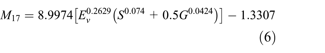
where E_v is the illuminance, S is the S-cone response normalised using relative light source SPD and G is the ipRGC response normalised using relative light source SPD, as shown in Equations (7) and (8)

$$S=\frac{\int P_{\mathrm{rel}}(\lambda )s_{\mathrm{sc}}\left(\lambda \right)d\lambda }{\int P_{\mathrm{rel}}(\lambda )V\left(\lambda \right)d\lambda }$$

(7)

$$G=\frac{\int P_{\mathrm{rel}}(\lambda )s_{\mathrm{mel}}\left(\lambda \right)d\lambda }{\int P_{\mathrm{rel}}(\lambda )V\left(\lambda \right)d\lambda }$$

(8)

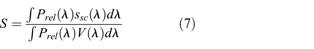
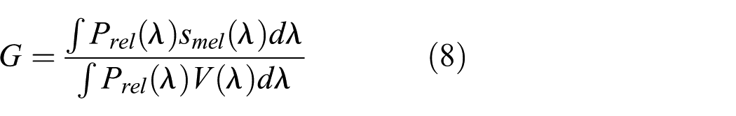
where P_rel(λ) is the relative SPD of the light source calculated using Equation (9)

$$P_{\mathrm{rel}}(\lambda )=\frac{P_{\mathrm{abs}}\left(\lambda \right)100}{\int P_{\mathrm{abs}}(\lambda )V\left(\lambda \right)\mathrm{d}\mathrm{\lambda }}$$

(9)

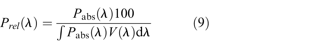
where P_abs(λ) is the absolute SPD (spectral irradiance) at the object level. Although Khanh et al. calculated M₁₇ from spectral irradiance at the object level, in this study the metric was derived from spectral irradiance at the observer’s eye level, as no physical objects were present in either experiment. However, to the authors’ knowledge, none of these melanopsin-based spatial brightness models (here, referred to as B, R and M₁₇ for brevity) have been independently assessed. This study evaluates the performance of the melanopsin-based spatial brightness metrics using data from two psychophysical experiments.

2. Methods

Two psychophysical experiments have been previously conducted to investigate the effects of melanopsin and colour gamut on spatial brightness. ²⁷ Here, the data from these visual experiments are analysed to test the performance of three spatial brightness metrics that account for the melanopsin contribution in visual mechanisms.

2.1 Experiment 1

2.1.1 Lighting conditions

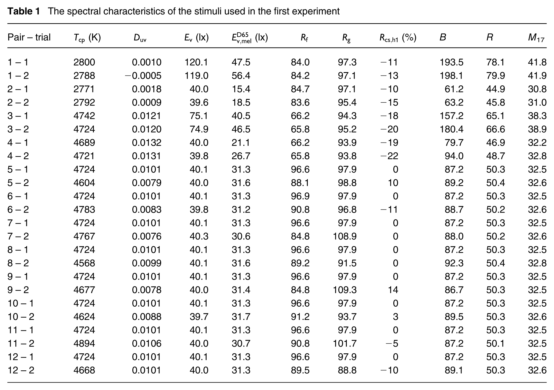
Twelve pairs of lighting conditions were generated using a multi-colour tuneable LED lighting system (LEDCubes, Thouslite) at two nominal CCT (2700 K and 4700 K) and three vertical illuminance (40 lx, 75 lx and 120 lx) levels at the eye level, as shown in Table 1. To account for the limitations of CCT, ³⁸ a spectral optimisation algorithm was used to generate the test stimuli targeted minimal differences in the CIE 1931 ( $x,y$ ) chromaticity coordinates. The CCT difference between trials was on average 15 K, and the maximum difference of 170 K was below the perceivable threshold. ³⁹ The SPD of the first two lighting trials in pair 1 are shown in Figure 1 as an example. The colorimetric and photometric characteristics of the lighting conditions were measured using a calibrated spectroradiometer (BTS256-EF, Gigahertz-Optik, Amesbury, USA). BTS256-EF measures spectral irradiance between 360 nm and 830 nm at 1 nm intervals with a repeatability of ±0.0002 for Δx and Δy, ±2% for ΔT_cp, and the illuminance calibration uncertainty is ±2.2%. ⁴⁰

Table 1

The spectral characteristics of the stimuli used in the first experiment

Pair – trial	$T_{\mathrm{cp}}$ (K)	$D_{\mathrm{uv}}$	$E_{\mathrm{v}}$ (lx)	$E_{\mathrm{v},\mathrm{mel}}^{\mathrm{D}65}$ (lx)	$R_{\mathrm{f}}$	$R_{\mathrm{g}}$	$R_{\mathrm{cs},\mathrm{h}}$ 1 (%)	B	R	M 17
1 – 1	2800	0.0010	120.1	47.5	84.0	97.3	−11	193.5	78.1	41.8
1 – 2	2788	−0.0005	119.0	56.4	84.2	97.1	−13	198.1	79.9	41.9
2 – 1	2771	0.0018	40.0	15.4	84.7	97.1	−10	61.2	44.9	30.8
2 – 2	2792	0.0009	39.6	18.5	83.6	95.4	−15	63.2	45.8	31.0
3 – 1	4742	0.0121	75.1	40.5	66.2	94.3	−18	157.2	65.1	38.3
3 – 2	4724	0.0120	74.9	46.5	65.8	95.2	−20	180.4	66.6	38.9
4 – 1	4689	0.0132	40.0	21.1	66.2	93.9	−19	79.7	46.9	32.2
4 – 2	4721	0.0131	39.8	26.7	65.8	93.8	−22	94.0	48.7	32.8
5 – 1	4724	0.0101	40.1	31.3	96.6	97.9	0	87.2	50.3	32.5
5 – 2	4604	0.0079	40.0	31.6	88.1	98.8	10	89.2	50.4	32.6
6 – 1	4724	0.0101	40.1	31.3	96.9	97.9	0	87.2	50.3	32.5
6 – 2	4783	0.0083	39.8	31.2	90.8	96.8	−11	88.7	50.2	32.6
7 – 1	4724	0.0101	40.1	31.3	96.6	97.9	0	87.2	50.3	32.5
7 – 2	4767	0.0076	40.3	30.6	84.8	108.9	0	88.0	50.2	32.6
8 – 1	4724	0.0101	40.1	31.3	96.6	97.9	0	87.2	50.3	32.5
8 – 2	4568	0.0099	40.1	31.6	89.2	91.5	0	92.3	50.4	32.8
9 – 1	4724	0.0101	40.1	31.3	96.6	97.9	0	87.2	50.3	32.5
9 – 2	4677	0.0078	40.0	31.4	84.8	109.3	14	86.7	50.3	32.5
10 – 1	4724	0.0101	40.1	31.3	96.6	97.9	0	87.2	50.3	32.5
10 – 2	4624	0.0088	39.7	31.7	91.2	93.7	3	89.5	50.3	32.6
11 – 1	4724	0.0101	40.1	31.3	96.6	97.9	0	87.2	50.3	32.5
11 – 2	4894	0.0106	40.0	30.7	90.8	101.7	−5	87.2	50.1	32.5
12 – 1	4724	0.0101	40.1	31.3	96.6	97.9	0	87.2	50.3	32.5
12 – 2	4668	0.0101	40.0	31.3	89.5	88.8	−10	89.1	50.3	32.6

Figure 1

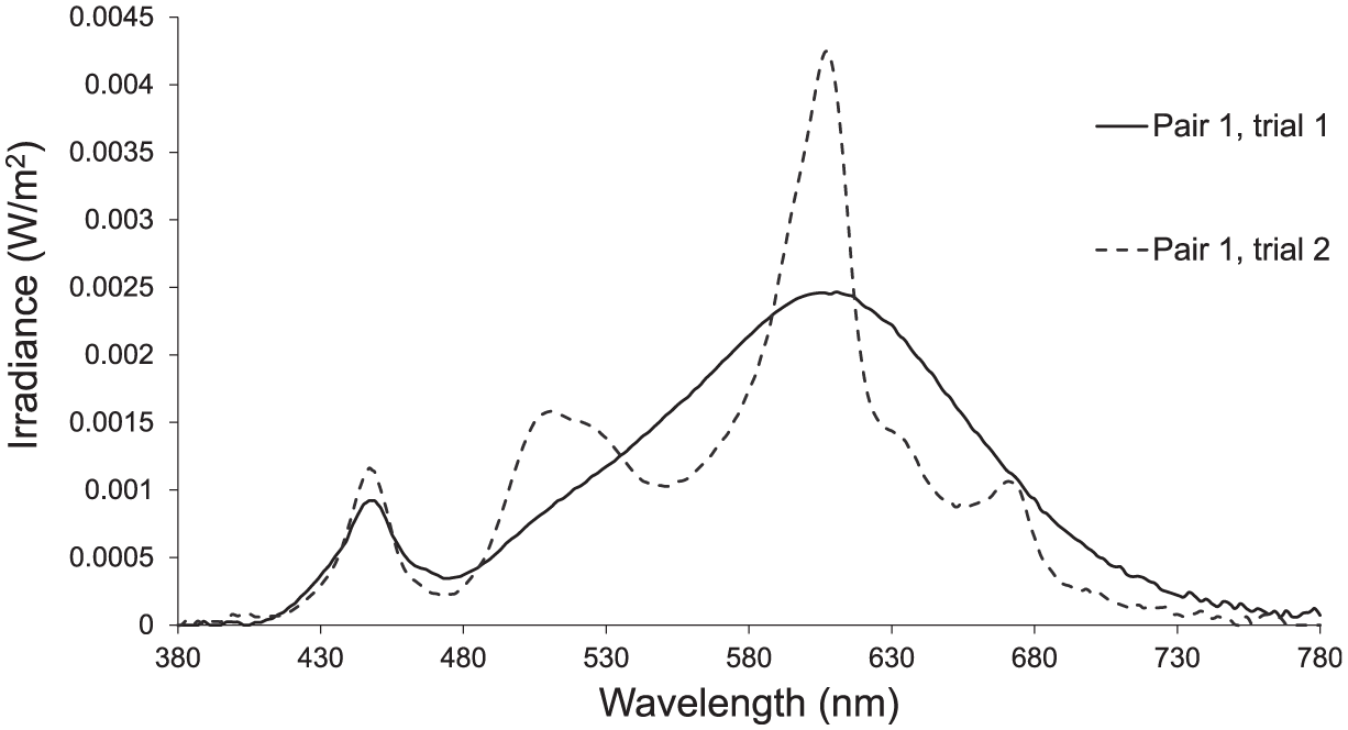
The SPD of the first two trials of pair one: pair 1 trial 1 (straight line) and pair 1 trial 2 (dashed line) from Table 1

2.1.2 Participants

A power analysis was conducted using G-power software, ⁴¹ and 42 participants (22 females and 20 males) with a median age of 26 (ranged between 19 years and 51 years) were recruited. Participants’ colour vision was tested by Ishihara pseudo-isochromatic colour deficiency test, visual acuity was tested by Snellen chart, and depth perception and binocular acuity were tested by Keystone visual skills test. Participants provided verbal consent prior to the experiment and were compensated for their time. An ethics approval was granted by the local institutional review board (IRB; STUDY00017315).

2.1.3 Experiment protocol

The experiment took place in a controlled laboratory where two neutrally painted, side-by-side rooms were utilised. The rooms were empty to control the effects of object colourfulness on brightness, such as the Hunt and Helmholtz–Kohlrausch effects, ⁴² as shown in Figure 2. Lighting conditions were generated and controlled using MATLAB^® (v2022b). Training and three null conditions were provided, and trials were randomised and counterbalanced to reduce biases, such as learning effect and anchoring bias. ⁴³ Position bias was accounted for by counterbalancing the stimulus shown on both right-hand side and left-hand side. ⁴⁴ A head-chin rest was used to stabilise participants’ visual field to control the effects of visual field and retinal position of stimuli on spatial brightness. ⁴⁵ Participants were asked to judge the spatial brightness of two side-by-side rooms lit simultaneously using a 2-alternative forced choice (2AFC) method where they chose the room that appeared brighter. Each pair was presented for 7 s before a judgement was made, as shown in Figure 3. There was a 0.5-s dark transition between pairs. The data were collected in the afternoons and evenings.

Figure 2

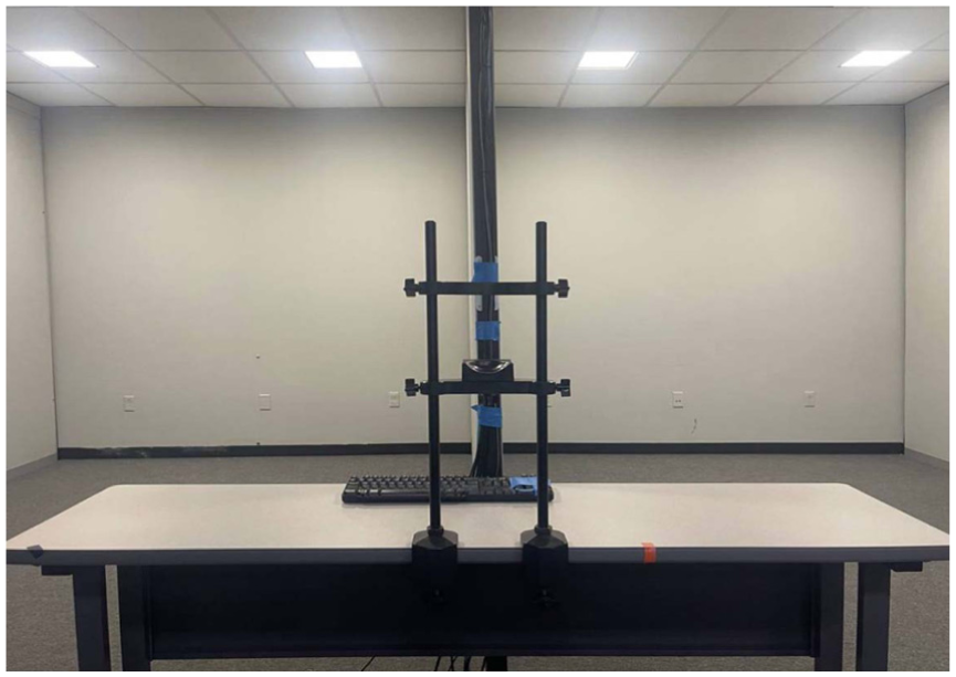
The experiment took place in neutrally painted side-by-side rooms, and a chin rest was used to stabilise participants’ visual field

Figure 3

Lighting conditions within a pair were shown for 7 s in side-by-side rooms, followed by a beep sound to encourage the participants to choose the brighter side. There was a 0.5-s dark transition before the next pair was shown

The experiment was conducted in two parts. In part 1, first four lighting pairs (1–1 to 4 – 2) were shown in a randomised order. In part 2, lighting condition 5 – 1 was compared to eight different lighting conditions that have the same illuminance, chromaticity and melanopic content. The goal was to enlarge the differences in ANSI/IES TM-30 gamut index (R_g) or red chroma shift in hue bin 1 (R_cs,h1). Each pair was repeated 10 times, resulting in 60 and 90 pairs respectively for parts 1 and 2, which included null conditions that were deployed to address position bias between left and right rooms. Participants were encouraged to respond at the end of the 7-s period with a beep sound. Otherwise they were free to look at the conditions longer, but their responses were mostly within a reasonable time (∼10 s). Between parts 1 and 2 there was a 5-min break to avoid visual fatigue.

2.2 Experiment 2

2.2.1 Lighting conditions

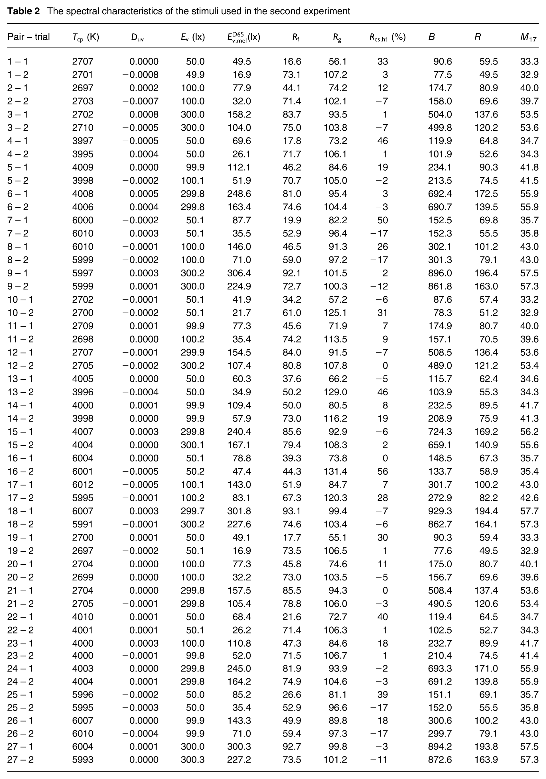
Twenty-seven pairs of lighting conditions were generated using the same multi-colour 15-primary LED lighting system (LEDCubes, Thouslite) at three nominal CCT (2700 K, 4000 K and 6000 K) and three vertical illuminance (50 lx, 100 lx and 300 lx) levels at the eye level, as shown in Table 2. The second experiment had similar bias reduction measures and measurement protocols. ²⁷

Table 2

The spectral characteristics of the stimuli used in the second experiment

Pair – trial	$T_{\mathrm{cp}}$ (K)	$D_{\mathrm{uv}}$	$E_{\mathrm{v}}$ (lx)	$E_{\mathrm{v},\mathrm{mel}}^{\mathrm{D}65}$ (lx)	$R_{\mathrm{f}}$	$R_{\mathrm{g}}$	$R_{\mathrm{cs},\mathrm{h}}$ 1 (%)	B	R	M 17
1 – 1	2707	0.0000	50.0	49.5	16.6	56.1	33	90.6	59.5	33.3
1 – 2	2701	−0.0008	49.9	16.9	73.1	107.2	3	77.5	49.5	32.9
2 – 1	2697	0.0002	100.0	77.9	44.1	74.2	12	174.7	80.9	40.0
2 – 2	2703	−0.0007	100.0	32.0	71.4	102.1	−7	158.0	69.6	39.7
3 – 1	2702	0.0008	300.0	158.2	83.7	93.5	1	504.0	137.6	53.5
3 – 2	2710	−0.0005	300.0	104.0	75.0	103.8	−7	499.8	120.2	53.6
4 – 1	3997	−0.0005	50.0	69.6	17.8	73.2	46	119.9	64.8	34.7
4 – 2	3995	0.0004	50.0	26.1	71.7	106.1	1	101.9	52.6	34.3
5 – 1	4009	0.0000	99.9	112.1	46.2	84.6	19	234.1	90.3	41.8
5 – 2	3998	−0.0002	100.1	51.9	70.7	105.0	−2	213.5	74.5	41.5
6 – 1	4008	0.0005	299.8	248.6	81.0	95.4	3	692.4	172.5	55.9
6 – 2	4006	0.0004	299.8	163.4	74.6	104.4	−3	690.7	139.5	55.9
7 – 1	6000	−0.0002	50.1	87.7	19.9	82.2	50	152.5	69.8	35.7
7 – 2	6010	0.0003	50.1	35.5	52.9	96.4	−17	152.3	55.5	35.8
8 – 1	6010	−0.0001	100.0	146.0	46.5	91.3	26	302.1	101.2	43.0
8 – 2	5999	−0.0002	100.0	71.0	59.0	97.2	−17	301.3	79.1	43.0
9 – 1	5997	0.0003	300.2	306.4	92.1	101.5	2	896.0	196.4	57.5
9 – 2	5999	0.0001	300.0	224.9	72.7	100.3	−12	861.8	163.0	57.3
10 – 1	2702	−0.0001	50.1	41.9	34.2	57.2	−6	87.6	57.4	33.2
10 – 2	2700	−0.0002	50.1	21.7	61.0	125.1	31	78.3	51.2	32.9
11 – 1	2709	0.0001	99.9	77.3	45.6	71.9	7	174.9	80.7	40.0
11 – 2	2698	0.0000	100.2	35.4	74.2	113.5	9	157.1	70.5	39.6
12 – 1	2707	−0.0001	299.9	154.5	84.0	91.5	−7	508.5	136.4	53.6
12 – 2	2705	−0.0002	300.2	107.4	80.8	107.8	0	489.0	121.2	53.4
13 – 1	4005	0.0000	50.0	60.3	37.6	66.2	−5	115.7	62.4	34.6
13 – 2	3996	−0.0004	50.0	34.9	50.2	129.0	46	103.9	55.3	34.3
14 – 1	4000	0.0001	99.9	109.4	50.0	80.5	8	232.5	89.5	41.7
14 – 2	3998	0.0000	99.9	57.9	73.0	116.2	19	208.9	75.9	41.3
15 – 1	4007	0.0003	299.8	240.4	85.6	92.9	−6	724.3	169.2	56.2
15 – 2	4004	0.0000	300.1	167.1	79.4	108.3	2	659.1	140.9	55.6
16 – 1	6004	0.0000	50.1	78.8	39.3	73.8	0	148.5	67.3	35.7
16 – 2	6001	−0.0005	50.2	47.4	44.3	131.4	56	133.7	58.9	35.4
17 – 1	6012	−0.0005	100.1	143.0	51.9	84.7	7	301.7	100.2	43.0
17 – 2	5995	−0.0001	100.2	83.1	67.3	120.3	28	272.9	82.2	42.6
18 – 1	6007	0.0003	299.7	301.8	93.1	99.4	−7	929.3	194.4	57.7
18 – 2	5991	−0.0001	300.2	227.6	74.6	103.4	−6	862.7	164.1	57.3
19 – 1	2700	0.0001	50.0	49.1	17.7	55.1	30	90.3	59.4	33.3
19 – 2	2697	−0.0002	50.1	16.9	73.5	106.5	1	77.6	49.5	32.9
20 – 1	2704	0.0000	100.0	77.3	45.8	74.6	11	175.0	80.7	40.1
20 – 2	2699	0.0000	100.0	32.2	73.0	103.5	−5	156.7	69.6	39.6
21 – 1	2704	0.0000	299.8	157.5	85.5	94.3	0	508.4	137.4	53.6
21 – 2	2705	−0.0001	299.8	105.4	78.8	106.0	−3	490.5	120.6	53.4
22 – 1	4010	−0.0001	50.0	68.4	21.6	72.7	40	119.4	64.5	34.7
22 – 2	4001	0.0001	50.1	26.2	71.4	106.3	1	102.5	52.7	34.3
23 – 1	4000	0.0003	100.0	110.8	47.3	84.6	18	232.7	89.9	41.7
23 – 2	4000	−0.0001	99.8	52.0	71.5	106.7	1	210.4	74.5	41.4
24 – 1	4003	0.0000	299.8	245.0	81.9	93.9	−2	693.3	171.0	55.9
24 – 2	4004	0.0001	299.8	164.2	74.9	104.6	−3	691.2	139.8	55.9
25 – 1	5996	−0.0002	50.0	85.2	26.6	81.1	39	151.1	69.1	35.7
25 – 2	5995	−0.0003	50.0	35.4	52.9	96.6	−17	152.0	55.5	35.8
26 – 1	6007	0.0000	99.9	143.3	49.9	89.8	18	300.6	100.2	43.0
26 – 2	6010	−0.0004	99.9	71.0	59.4	97.3	−17	299.7	79.1	43.0
27 – 1	6004	0.0001	300.0	300.3	92.7	99.8	−3	894.2	193.8	57.5
27 – 2	5993	0.0000	300.3	227.2	73.5	101.2	−11	872.6	163.9	57.3

2.2.2 Participants

In the second experiment, a different group of 42 participants (18 females and 24 males) with a median age of 26 (ranged between 19 years and 56 years) were recruited. Participants’ colour vision was tested by Ishihara pseudo-isochromatic colour deficiency test, visual acuity was tested by the Snellen chart, and depth perception and binocular acuity were tested by the Keystone visual skills test. Participants provided verbal consent prior to the experiment and were compensated for their time. An ethics approval was granted by the local IRB (STUDY00017315).

2.2.3 Experiment protocol

The experiment took place in the same laboratory, but instead of using the two side-by-side rooms, only single room was utilised. A head-chin rest was used to stabilise participants’ visual field to control the effects of visual field and retinal position of stimuli on spatial brightness. ⁴⁵ The data were collected in the afternoons. Lighting conditions were generated and controlled using MATLAB^® (v2022b).

Participants were asked to judge the spatial brightness of a room using a 2-interval forced choice (2IFC) method. Each lighting condition was presented for 1 s with a 1 s dark transition between pairs, as shown in Figure 4. After the trial pairs were shown, participants made their judgement (chose the brighter condition) during a 3-s dark transition period. Each pair was repeated six times in a randomised order for each participant and counterbalanced within each section to address order bias. ⁴⁴ Lighting conditions of the same CCT were shown in the same section to allow full chromatic adaptation. ⁴⁶ For example, all the stimuli pairs that were 2700 K were shown within the same section. Therefore, there were three sections (2700 K, 4000 K and 6000 K) in total. The experiment lasted around 40 min in total and was divided into three sections with 5-min breaks between sessions to reduce visual fatigue. ⁴⁷

Figure 4

Pair of lighting conditions of the same CCT were shown in the same section. Each section started with a 5-min adaptation period, which also served as a break to reduce visual fatigue. Each trial within a pair were shown for 1 s, and there was a 1-s dark transition between the conditions in each pair. Participants chose the brighter conditions during the 3-s dark transition period at the end of each pairs

2.3 Statistical analysis

The data generated in these two experiments were analysed using parametric tests, as quantile–quantile (Q–Q) plots verified the normal distribution of the mean differences among the responses for the pairs. Since the responses were categorised as either ‘1’ or ‘2’, a binomial test was conducted for each comparison. For each experiment, the predictive performance of the spatial brightness metrics was evaluated by correlating the pair-wise mean subjective brightness proportion with each metric’s pair-wise difference. The Pearson’s r (with 95% confidence intervals (CIs) from Fisher’s z-transform), ordinary least squares slope (with 95% CIs), R² and two-sided p-values were reported. The significance level was established at α = 0.05. Within each experiment, p-values across the three metric tests were adjusted using the Holm–Bonferroni method. The Benjamini–Hochberg (BH) false discovery rate (FDR) was also computed as a sensitivity analysis. All the analysis was performed in MATLAB^® (v2019b).

The differences in metrics between trials of each pair were calculated and normalised to the maximum value of that metric. For example, the normalised difference for the B metric (dB_norm) for each pair was calculated using Equation (10)

$$\mathrm{d}{B}_{\mathrm{norm}}=\frac{(B_{i-j}-B_{i-j+1})}{B_{\max }}$$

(10)

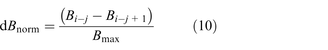
where i is the pair number, j is the trial number and B_max was the maximum value for that metric within each experiment. For example, the maximum value B_max was 198.1 for experiment 1 and 929.3 for experiment 2. The normalised difference for metrics R and M₁₇ (dR_norm and dM_17,norm, respectively) was also calculated. The maximum value R_max was 78.1 for experiment 1 and 196.4 for experiment 2. The maximum value M_17,max was 41.9 for experiment 1 and 57.7 for experiment 2.

3. Results

3.1 Experiment 1

Firstly, null conditions (presentation of two identical stimuli) were analysed to account for position bias. The responses to the 2800 K null conditions were 49% and 51% for right and left (p = 0.387) suggesting there was no position bias (no difference between left or right side of the room). One of the 4700 K null condition responses were 50% for both rooms (p = 0.780), but the other was 54% for right and 46% for left, with a significant difference (p = 0.013). Therefore, all pairs were counterbalanced in the left and right rooms to address position bias.

In most conditions, melanopsin-based spatial brightness metrics’ performance did not exceed 50% (coincidence). Regression analysis showed low explanatory power with R² values below 0.11 for all metrics, as shown in Figure 5. Among the three metrics, dB_norm exhibited the highest correlation (r = 0.325) and R² (0.106), followed by dM_17,norm and dR_norm, though differences were minimal and not statistically meaningful. Associations between subjective brightness and normalised metric differences were small and not statistically significant (dB_norm: slope = 15.73 percentage points (pp) per 1.0 dB_norm (95% CI: −16.50, 47.97), R² = 0.106, p = 0.302; Holm-adjusted p = 0.907; BH-adjusted p = 0.406; dR_norm: slope =  8.81 pp per 1.0 dR_norm (95% CI: −13.83, 31.45), R² = 0.070, p = 0.406; Holm-adjusted p = 0.907; BH-adjusted p = 0.406; dM_17,norm: slope = 12.84 pp per 1.0 dM_17,norm (95% CI: −15.59, 41.27), R² = 0.092, p = 0.338; Holm-adjusted p = 0.907; BH-adjusted p = 0.406). No test reached significance after multiplicity control (Holm or FDR). Overall, data from experiment 1 showed limited predictive accuracy for all three melanopsin-based metrics.

Figure 5

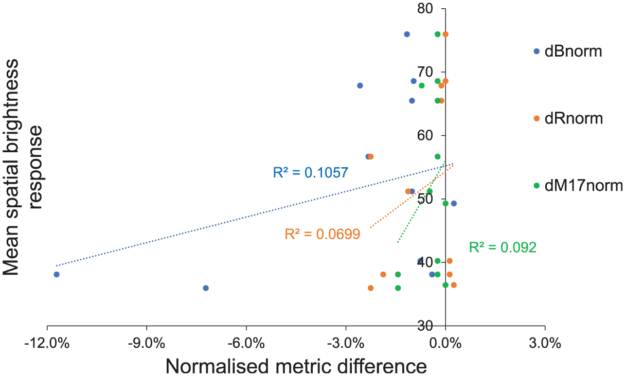
Subjective spatial brightness responses (y-axis) in experiment 1 against metric differences (x-axis). The differences in melanopsin-based metrics were normalised to their maximum using Equation (10) to allow comparison across scales. Negative values indicate that the metric predicts the second condition in a pair would appear brighter. The error bars represent the standard error of the mean for subjective spatial brightness responses. The dotted lines are the linear regression lines, and R ² is the correlation coefficient.

3.2 Experiment 2

The analysis of the data from experiment 2 revealed only a weak to moderate correlations between subjective spatial brightness ratings and the melanopsin-based metrics. dR_norm exhibited the strongest relationship (r = −0.439, p = 0.022), indicating a statistically significant but negative association with spatial brightness. In contrast, dB_norm and dM_17,norm showed weak correlations (r = −0.216 and r = 0.205, respectively) with p-values above 0.28, suggesting no significant predictive capability. These results indicate that, overall, melanopsin-based metrics do not consistently align with subjective spatial brightness judgements under the tested conditions.

Regression analysis further confirmed these findings, with R² values remaining low across all metrics, indicating limited explanatory power. dR_norm achieved the highest R² (0.192), while dB_norm and dM_17,norm accounted for less than 5% of the variance in subjective ratings, as shown in Figure 6. Interestingly, the negative slope for dR_norm suggests that higher metric values corresponded to lower spatial brightness, contrary to expectations. Using normalised metric differences, one metric showed a modest unadjusted association that did not survive multiplicity control (dB_norm: slope = −110.14 pp per 1.0 dB_norm (95% CI: −315.38, 95.09), R² = 0.047, p = 0.280; Holm-adjusted p = 0.559, BH-adjusted p = 0.306; dR_norm: slope = −93.87 pp per 1.0 dR_norm (95% CI: −173.07, −14.67), R² = 0.192, p = 0.022; Holm-adjusted p = 0.066, BH-adjusted p = 0.066; dM_17,norm: slope = 548.16 pp per 1.0 dM_17,norm (95% CI: −531.46, 1627.78), R² = 0.042, p = 0.306; Holm-adjusted p = 0.559, BH-adjusted p = 0.306). Thus, no metric remained significant after Holm–Bonferroni adjustment in experiment 2. The unadjusted negative association for dR_norm suggests that larger normalised R metric differences were linked to a lower probability that the first condition was judged brighter, but the effect was not robust to multiplicity control. Collectively, these results highlight that melanopsin-weighted approaches, while physiologically relevant, did not provide accurate predictions of spatial brightness in this experiment.

Figure 6

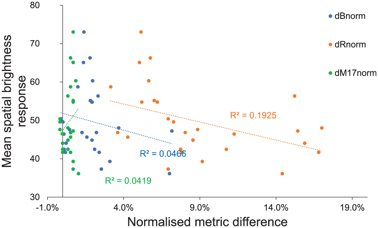
Subjective spatial brightness responses (y-axis) in experiment 2 against metric differences (x-axis). Melanopsin-based metric changed were normalised to their maximum using Equation (10) to allow comparison across scales. Negative values indicate that metric predicts the second condition in a pair would appear brighter. The error bars represent the standard error of the mean for subjective spatial brightness responses. The dotted lines are the linear regression lines, and R ² is the correlation coefficient

The observed differences in predictive performance among the three melanopsin-based metrics can be explained by their underlying formulations. The B metric incorporates photopic illuminance, S-cone sensitivity and melanopsin stimulation, with a logarithmic term for vertical illuminance that amplifies the S-cone contribution at higher light levels. This structure makes B more responsive to both illuminance and short-wavelength content. Similarly, the R metric combines melanopsin stimulation and luminance with a pupil diameter adjustment, introducing non-linearity that reflects physiological adaptation to light. These features allow B and R to vary meaningfully with melanopic contribution, but not necessarily improve their alignment with subjective spatial brightness judgements.

In contrast, the M₁₇ metric exhibits minimal sensitivity to spectral composition and melanopsin activation. Its formula is dominated by illuminance raised to a modest exponent (0.2629), while S-cone and ipRGC contributions are scaled by very small exponents (0.074 and 0.0424). This dampens the influence of spectral differences, resulting in predictions that remain relatively constant across conditions with similar illuminance. Consequently, M₁₇ fails to capture perceptual spatial brightness variations in scenes where spectrum plays a significant role, explaining its weaker correlation with subjective ratings compared to B and R.

If melanopsin-based spatial brightness metrics are normalised to their maximum to account for the fact that they have different scaling factors (i.e. the maximum values of each metric are not necessarily the same), their predictions can be compared to Stevens power law, as shown in Figure 7. Here, M₁₇, B and R continue to exhibit linear responses to increasing light levels. Their responses to spectral changes (low and high CCT shown at top and bottom graphs, respectively) are minimal and similar in direction and magnitude. Finally, it is likely that neither Stevens’ power law nor ‘Weber–Fechner’ law are perfect estimates for spatial brightness. The predictive performance of power and logarithmic estimation of spatial brightness is beyond the scope of this study (which requires a different experimental protocol), but definitely worth investigating in the future.

Figure 7

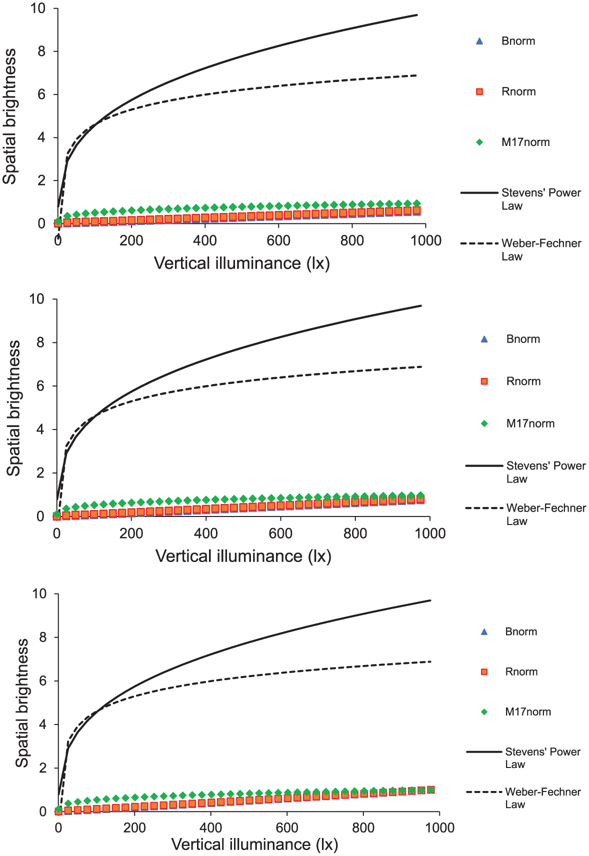
Normalised melanopsin-based spatial brightness metrics (dB_norm = blue triangle, dR_norm = red square and dM_17,norm = green diamond) and subjective brightness predictions calculated using Stevens’ power law (continuous line) and Weber–Fechner law (dotted line) for 2700 K (top), 4000 K (middle) and 6000 K (bottom) as a function of vertical illuminance (x-axis)

4. Discussion

The weak associations found in these two experiments imply that melanopsin-weighted spatial brightness metrics, while physiologically motivated, may not capture the spectral dimension of spatial brightness under the experimental conditions used. The poor performance of the melanopsin-based metrics may have been caused by overfitting of data used in the originating experiments where a larger range of illuminance, melanopsin response or chromaticity values were utilised. While a mathematical model that has an applicability to a wide range of values may be useful for general use, the studied metrics have low explanatory power that does not provide insight into the mechanistic role of melanopsin in spatial brightness.

The findings raise important questions about whether spatial brightness can be fully explained by melanopsin-based models or if a return to multi-stage colour vision theory ⁴⁸ is warranted. Traditional models emphasise the combined contributions of cone cells (primarily L- and M-cone cell response), but the combination of photopic, S-cone and ipRGC pathways, which interact across multiple stages of visual processing, should be further investigated. The relatively weak performance of melanopsin-based metrics suggests that spatial brightness may not be governed by a single photoreceptor class but rather by an integrated response involving both spectral and spatial cues. This aligns with theories that spatial brightness is a multidimensional construct influenced by luminance, chromatic adaptation and physiological factors, such as pupil size.

Another critical factor in spatial brightness is the distribution of light within a space. Although these experiments controlled intensity distribution to focus on spectral effects, prior research indicates that spatial factors – such as the relative luminance of walls, ceilings and floors^49,50– play a dominant role in spatial brightness. Metrics, such as Feu ⁵¹ or mean room surface exitance, ⁵² have been used to account for these spatial components, reflecting the idea that brightness is not solely a spectral phenomenon but a spatial one – hence the name ‘spatial’ brightness. Given that architectural lighting often prioritises uniformity and surface luminance,^53,54 it is reasonable to assume that spatial distribution exerts a stronger influence on brightness than spectral composition alone.

To recap, spatial brightness in this paper refers to the perceived overall brightness of an extended scene under a given lighting condition, distinct from photometric measures. Our understanding, as a reflection of the current literature, is that spatial brightness depends on spatial organisation and contrast (lightness and surround effects), spectral content (including colour appearance phenomena such as Helmholtz–Kohlrausch ⁵⁵ and Hunt effects ⁵⁶ ) and temporal factors (summation and adaptation). Consequently, in complex scenes, the visual system often trades off or ‘normalises’ these cues, ⁵⁷ making differences in brightness harder to detect in some contexts (e.g. in a room full of objects). In addition, stimuli characteristics (i.e. visual angle ⁴⁵ and retinal position ⁵⁸ ) and observer viewing configurations (fixation position ⁵⁹ ) can be particularly influential. For example, fixation position reflects the importance of central vision over peripheral vision, which is clearly demonstrated by the cone photoreceptor distribution in the retina. Taken together, this suggests that any practical model of spatial brightness must be multidimensional – jointly accounting for the scene’s spatial structure, spectral composition and temporal viewing conditions – beyond photopic luminance, vertical illuminance or melanopic contribution alone.

It is also important to acknowledge the limitations of the study. The participants were asked to judge the brightness of the space in each experiment, but Boyce et al. argued that the participants should be asked to judge not only the brightness of the space but also the lightness of the surfaces, ⁶⁰ which requires providing definitions of lightness and brightness to participants. In addition, the stimuli were optimised to test melanopsin contributions rather than to systematically evaluate the full range of spatial brightness models. Illuminance levels were not broadly varied, and the spectral differences were constrained to maintain control over other variables. While this approach was necessary to isolate melanopsin effects, it limits the generalisability of the findings to real-world lighting scenarios where illuminance and spectral composition vary widely. When generating the stimuli, the CIE 2° colour matching functions (CMFs) were used to calculate CCT and chromaticity coordinates, which reflect a smaller FOV compared to 10° CMFs. The chromaticity difference Δ(x, y) between 2° and 10° CMFs was 0.0172 with a standard deviation of 0.012, highlighting the impact of FOV as noted in previous studies.^7,9

In addition, stimulus duration and receptor time courses can also impact spatial brightness. Spatial brightness judgements likely reflect the combined activity of fast cone pathways and slower ipRGC signals, which integrate over longer timescales. Cone channels responses show short-latency and develop well within a 1-s exposure. ⁶¹ In contrast, ipRGC responses exhibit longer latencies (hundreds of milliseconds), slower dynamics and sustained post-stimulus activity, ⁶² implying that longer presentations (e.g. 7 s) are more conducive to capturing melanopsin-mediated contributions than brief ones (e.g. 1 s). Accordingly, the temporal structure of the stimuli used in these two experiments may have differentially weighted cone – versus ipRGC-driven signals – the use of 1-s versus 7-s presentations likely biased the balance between fast cone pathways and slower ipRGC signals. A recent study found reduced but significant effects of spectra on spatial brightness between a 5-s and 20-min viewing time. ⁶³ In sum, a systematic investigation of the effect of a wide range of exposure durations on spatial brightness is needed.

4. Conclusions

Spatial brightness, a term relevant for architectural lighting research and design, is gaining recognition, yet a robust quantification method is still needed. While currently there is no universally agreed spatial brightness model, the term spatial brightness has been championed to overcome the limitations of standard photometry in predicting brightness, especially due to small FOV and exclusion of photoreceptor responses beyond L- and M-cones. More recent studies also indicate ipRGCs, another type of photoreceptor in the retina, might be contributing to visual pathways. To address these intriguing research questions, two psychophysical experiments were conducted to evaluate the effects of melanopsin and colour gamut on spatial brightness. The experimental data were used to test the performance of specialised spatial brightness models based on melanopsin contributions.

The results of the experiments suggest that explanatory power of spatial brightness models is low. Future studies should use datasets with large illuminance and CCT ranges to test the predictive power of these models. Future experiments can also utilise stimuli specifically generated to identify the differences between these metrics. Nonetheless, the results suggest the need to develop more robust melanopsin-based spatial brightness models, not necessarily to predict occupants’ responses in a broad set of conditions, but to expand explanatory breadth of these models. ⁶⁴ Such new models can be theory-driven rather than data-driven to explore the working principles of the integrated human visual and non-visual responses. Theory-driven spatial brightness models can also help identify a threshold for the spectral dimension of spatial brightness.