Revision of M P calculation method for flicker measurement

Abstract

Direct flicker is a perception effect causing discomfort generated from lighting systems. While the short-term flicker indicator, $P_{\mathrm{st}}^{\mathrm{LM}}$ , is most widely used, perceptual modulation (M_P) is also a perception-based direct flicker metric used in many commercial instruments. However, M_P values show substantial variation due to different starting phases of waveforms, caused by Fourier transform spectral leakage. Such variation was mostly removed by revising M_P’s calculation, applying a Hann window function and a correction factor to counteract the spectral broadening from the window when summing the DC-normalized spectral components. This approach is generalized to improve frequency-domain temporal light artefact metrics without loss of perceptual relevance when different windows are applied. To harmonize M_P with direct flicker at a broader frequency range and viewing conditions eliciting higher direct flicker sensitivity, its original sensitivity curve (5 Hz to 65 Hz) is replaced by the one from Perz’s experiment, with a slight change of frequency range to 3 Hz to 80 Hz. With these improvements, M_P,26 has been developed. A linear mixed-effects model is used to compare the different measurement conditions of M_P,26, providing guidance for recommended measurement conditions, i.e. measurement duration ≥5 s, sampling rate ≥2 kHz and a second-order anti-aliasing filter with cut-off frequency ≥400 Hz are recommended for robust result of M_P,26.

1. Introduction

Temporal light modulation (TLM), variations in the light intensity or spectral distribution as a function of time, is present in almost all lighting systems including solid-state light sources. Inadequate selection of drivers for lamps or dimmers, and compatibility problems between the connected electrical components can lead to noticeable temporal light artefacts (TLAs), such as direct flicker or stroboscopic effects. TLA refers to the visible portion of TLM responses, i.e., those that can be perceived by the human eye, while TLM responses encompass the full range of temporal responses, including both visible and non-visible effects, which may have physiological impacts even if they are not directly perceptible. Direct flicker, as an important perceptual effect, is defined as the direct perception of temporal changes in light output with a steady gaze. It is considered a type of TLA that may cause unwanted discomfort or health problems.^1–5 The direct flicker effect is common in everyday life, which has been widely observed in products from LED holiday light strings to lamps.

The availability of direct flicker metrics, their ease of use, and measurement uncertainty are important for product characterization. Short-term flicker indicator, $P_{\mathrm{st}}^{\mathrm{LM}}$ , defined in IEC TR 61547-1, ⁶ is the most widely used direct flicker metric, now used in Ecodesign regulation in Europe (EU, 2019). Perceptual modulation, M_P, published by ASSIST ⁷ is another direct flicker metric often used in commercial instruments.

Recently, to validate the consistency of TLM measurements and to investigate the measurement uncertainty of TLM quantities, the International Energy Agency (IEA) 4E Solid-State Lighting Annex organized an Interlaboratory Comparison of TLM Measurements of Solid-State Lighting (SSL) Products (IC 2023),^8,9 which evaluated direct flicker metrics, $P_{\mathrm{st}}^{\mathrm{LM}}$ and M_P, as well as the stroboscopic effect visibility measure (SVM, symbol M_vs) and other metrics.^10,11

$P_{\mathrm{st}}^{\mathrm{LM}}$ was originally developed to evaluate the power line quality by predicting incandescent lighting flicker based on the AC voltage waveform instead of direct measurement of the light waveform. Though $P_{\mathrm{st}}^{\mathrm{LM}}$ has been adapted from the original P_st by direct use of the light waveform in the calculation, $P_{\mathrm{st}}^{\mathrm{LM}}$ was designed to measure not only flicker generated by the light source but also the power line voltage fluctuations, which is also important for evaluation of flicker in real applications. Thus, measurement of $P_{\mathrm{st}}^{\mathrm{LM}}$ requires 180 s measurement duration. However, this is causing significant variations in measurement. It was revealed in the IEA interlaboratory comparison ⁹ that there were significant variations in $P_{\mathrm{st}}^{\mathrm{LM}}$ measurements due to different power supplies used to operate the LED lamps measured. In addition, in a recent paper by Li and Ohno, ¹² substantial variations in $P_{\mathrm{st}}^{\mathrm{LM}}$ were found for different measurement durations or sampling rates for certain test waveforms.

The M_P metric uses a calculation method in the frequency domain with shorter measurement time (several seconds), similar to that used in SVM. ¹¹ Specifically, the M_P metric uses the relative light waveform as input, weights the DC-normalized Fourier transform (FT) spectral components of the waveform using a perceptual sensitivity weighting function based on experimental data from human vision and sums them in quadrature to derive a metric that predicts the degree of perceived visible modulation. ¹³ As the M_P metric was designed to measure flicker solely from the luminous output of a lamp, and is not necessarily concerned with power line disturbances, it requires a much shorter measurement time (∼2 s) compared to 180 s in $P_{\mathrm{st}}^{\mathrm{LM}}$ .^14,15

$P_{\mathrm{st}}^{\mathrm{LM}}$ and M_P are both direct flicker metrics, but they serve different purposes and have distinct characteristics: $P_{\mathrm{st}}^{\mathrm{LM}}$ is intended for assessing the acceptability/severity of power line disturbances and does not address the psychophysical detection of flicker, while M_P is designed to detect direct flicker on a much shorter time scale, without considering the acceptability of recurring flicker events.

M _P can evaluate the flicker from the lamp alone, allowing reproducible measurements with low uncertainties, and is thus suitable for testing of lighting products. However, large variations in M_P measurements were observed in IC 2023. ⁹ Thus, the aim of this study is to investigate the causes of the measurement variations in M_P and to improve the calculation method of the M_P metric to provide more robust results. Our investigation revealed that the M_P calculation method is very sensitive to how the waveform was digitally acquired. It was found that different measurement conditions (e.g. measurement duration, starting phase of waveform, sampling rate) can have a significant impact on the M_P value. The experimental analysis on this aspect is discussed in Section 2.

In addition, the choice of the frequency range of the direct flicker sensitivity function is critical for perceptual relevance of the results. Based on the IEEE 1789 Standard on LED Lighting Flicker and Potential Health Concerns, risks of seizures due to flicker at frequencies are considered within the range of about 3 Hz to 70 Hz.^16,17 The temporal contrast sensitivity function (TCSF) is used to characterize the relation between flicker visibility and temporal frequency. De Lange ¹⁸ and Kelly^19,20 measured TCSFs using different visual fields, for several retinal illuminance levels. In 2015, the perceptual modulation (M_P) flicker metric was developed at the Lighting Research Center based on Bodington’s visual data. ⁷ The total perceived modulation is calculated as the square root of the sum of the squares of the perceptual frequency components. The component perceptual strengths are calculated by dividing the modulation amplitudes (A_k, where k indicates the kth frequency component) by the DC level (A₀) for Weber–Fechner law scaling, and dividing by the modulation detection threshold (M_DTH,k) value for each frequency, as indicated in Equation (1). ⁷

$$M_{\mathrm{P}}=\sqrt{\sum _{k=1}^{\infty }\frac{A_k^2}{A_0{M}_{\mathrm{DTH},k}^2}}$$

(1)

The experiment of Bodington et al. ¹³ was conducted in central vision, by directly observing a 600-lumen A-lamp (7° visual angle) illuminating a light grey background (∼90° viewing field, ∼3000 K, 20 cd m⁻² to 200 cd m⁻²). The resultant metric is most applicable for emission measurements, i.e. product characterization. The direct flicker sensitivity curve of M_P covers a frequency range 5 Hz to 65 Hz, slightly narrower than the IEEE recommended risky frequency range of ∼3 Hz to ∼70 Hz.^16,17

In 2017, Perz et al. ²¹ conducted another direct flicker experiment using a diffused stimulus covering both peripheral and central vision (large visual field ∼120°), at high correlated colour temperature (CCT of 6500 K) and high luminance level (209 cd m⁻²). They found that direct flicker can be observed at more than 80 Hz. Based on these data, in 2017, the flicker visibility measure (generally referred to as FVM) was developed by Perz et al., ²¹ with a mathematical definition similar to that of M_P, calculated as a squared summation of the DC-normalized modulation of each frequency component ( $C_k)$ , normalized by the modulation detection threshold at the corresponding frequency ( $T_k)$ , as shown in the expression in Equation (2).

$$\sqrt{\sum _{k=1}^{\infty }\frac{C_k^2}{T_k^2}}$$

(2)

One point worth noting is that both M_P and the flicker measure of Perz et al. did not employ windowing techniques to guard against spectral power leakage in their calculations. Converting a time-domain sampled waveform to a power spectrum in the frequency domain by way of a discrete Fourier transform (DFT) assumes that the measured signal is one full or multiple full cycles of a periodic signal. Thus, for the DFT, both the time and frequency domains are circular topologies, and the two ends of the measured signal are assumed to be connected. When the measured waveform signal has an integer number of cycles, the DFT result is correct as the assumption is satisfied. However, when the measured signal does not have an integer number of cycles, the truncated waveform of the measured signal has different characteristics than the original continuous time-domain signal that are generated by the introduction of a sharp transition change to the time-domain signal where the two ends of the measured signal meet. This sharp transition change, or artificial discontinuity, appears in the DFT as additional frequency content that does not exist in the original signal. This can look as if the energy of the dominant frequency of the signal is leaking into other frequency regions, and so it is called spectral leakage. ²² A windowing technique is an established method and is often used in digital signal processing to improve this spectral leakage issue; it consists of multiplying the time-domain signal by a set of numerical weights the same length as the signal, called a window, with the amplitude peaked at the centre with a value of 1 and gradually decreasing symmetrically towards zero at the edges of the window. ²² The window introduces additional spectral components to the original FT spectrum while reducing overall spectral power, so a correction factor is needed to ensure the consistent scale of the result and maintain the perceptual relevance of the direct flicker measure. The ‘window + correction factor for integrated spectral power’ method presented in this paper will not only benefit the M_P metric but also the other TLA measures working in the frequency domain, such as Perz et al.’s FVM. The windowing technique has been implemented in SVM (M_vs),^11,23,24 but it seems that the correction factor used in M_vs does not fully address the integration of spectral power when an additional windowing function is applied to the waveform data. Instead, it appears to scale the peak amplitudes to match the values from the rectangular-windowed approach. Since window functions can affect the spectral amplitude distribution in various ways beyond just the peak amplitude (such as spectral peak broadening), it might be necessary to consider a correction factor that accounts for the integrated spectral power, rather than just the peak amplitudes, when working with frequency-domain metrics like M_P and Perz et al.’s FVM. In the case of M_vs, the correction factor used with ‘findpeaks()’, a MATLAB function employed in the normative MATLAB script provided by the IEC to compute this metric, may serve as a workaround. ¹¹ However, this approach does not fully account for the changes in integrated spectral power introduced by windowing. A correction factor explicitly designed to compensate for these spectral power integration effects is not included in the current implementation. This omission results in an incomplete correction from a spectral energy standpoint.

In this current study, the original M_P is revised by adding a Hann window and the above correction factor, and its performance is evaluated. The light waveforms of 11 typical commercial lamps, including 10 LED lamps and one compact fluorescent lamp (CFL), are measured using our customized measurement system at the National Institute of Standards and Technology (NIST). The M_P values are first calculated for the measured waveform at different durations and different starting phases using the MATLAB script included in the ASSIST document ⁷ and then recalculated using the revised M_P calculation method, M_P,26, to verify that the revision significantly improves M_P reproducibility. To broaden the scope of application of the M_P metric, the sensitivity curve in the original M_P is replaced by Perz’s sensitivity curve, ²¹ which has a higher sensitivity and a broader frequency range than the original sensitivity curve. Furthermore, an extensive statistical analysis is conducted to give recommendations on measurement duration, sampling rate and the anti-aliasing filter settings, by comparing the statistical variations in M_P,26 measured under different conditions. Finally, the performance of the M_P,26 metric and the recommended measurement conditions are validated using the measured waveforms of the 11 commercial lamps. This study presents a general method, referred to as the ‘window + correction factor’ method, to improve TLA metrics (particularly M_P) implemented in the frequency domain, and a novel method using statistical variations to reveal the effects of different waveform acquisition conditions (e.g. sampling frequency and duration) on TLA metric calculation. Both these methods can be utilized in best-practice recommendations and in regulations and standards for direct flicker evaluation. The MATLAB code for the M_P,26 metric is available in Supplemental Material associated with this paper.

2. Variations in measurement results of the original M_P

In the current study, the waveforms of light filtered by a V(λ) filter from a total of 11 different lamps (60 Hz AC power operation), including 7 relatively new LED lamps, 3 several year-old LED lamps and 1 CFL, were measured using a photodiode with a built-in amplifier, an anti-aliasing filter (commercial active low-pass filter) and sampled with a commercial high-speed digitizer (maximum sample rate of 20 MHz). The details of the tested lamps, including technical data, time and place of purchase, are given in Table A1. All the lamps were stabilized for 30 min before the measurements. The waveforms measured with the anti-aliasing filter are shown in Figure 1. The measurement duration for all waveforms was 180 s. The 10 LED lamps are indicated as ‘Lamp 1’ to ‘Lamp 10’, and the CFL is shown as ‘Lamp 11’.

Figure 1

Normalized waveforms of the 11 lamps. Waveforms were measured in the laboratory using a cut-off filter at 1 kHz with a 12 dB/octave roll-off and digitized at a 50 kHz sampling rate. Lamps 1 to 7 represent the 7 new LED lamps, Lamps 8 to 10 represent the 3 relatively old LED lamps and Lamp 11 represents the CFL

To investigate the impact of the waveform duration on the M_P values, the measured waveforms were cut into different segments of different durations, varying from 1 s to 180 s, always starting from the beginning of the measured waveforms. The waveforms used for the M_P calculation were filtered by an anti-aliasing analogue filter with a cut-off frequency at 1 kHz and a roll-off of 12 dB/octave, sampled at 50 kHz. The M_P values of the waveforms at different durations were calculated for each lamp and plotted as solid lines in Figure 2. Relatively large variations in M_P values can be observed for most lamp waveforms, due to different measurement durations. To compare, the M_P,26 values calculated using the revised method and the waveforms measured at the recommended conditions described in the following sections (filtered at a cut-off frequency at 1 kHz and a roll-off of 12 dB/octave, sampled at 10 kHz) were plotted in the same figure as dashed lines. As can be observed, the variations of M_P,26 values are reduced to within 0.01 for all 11 lamps, when using waveforms measured over 6 s as recommended in the following sections.

Figure 2

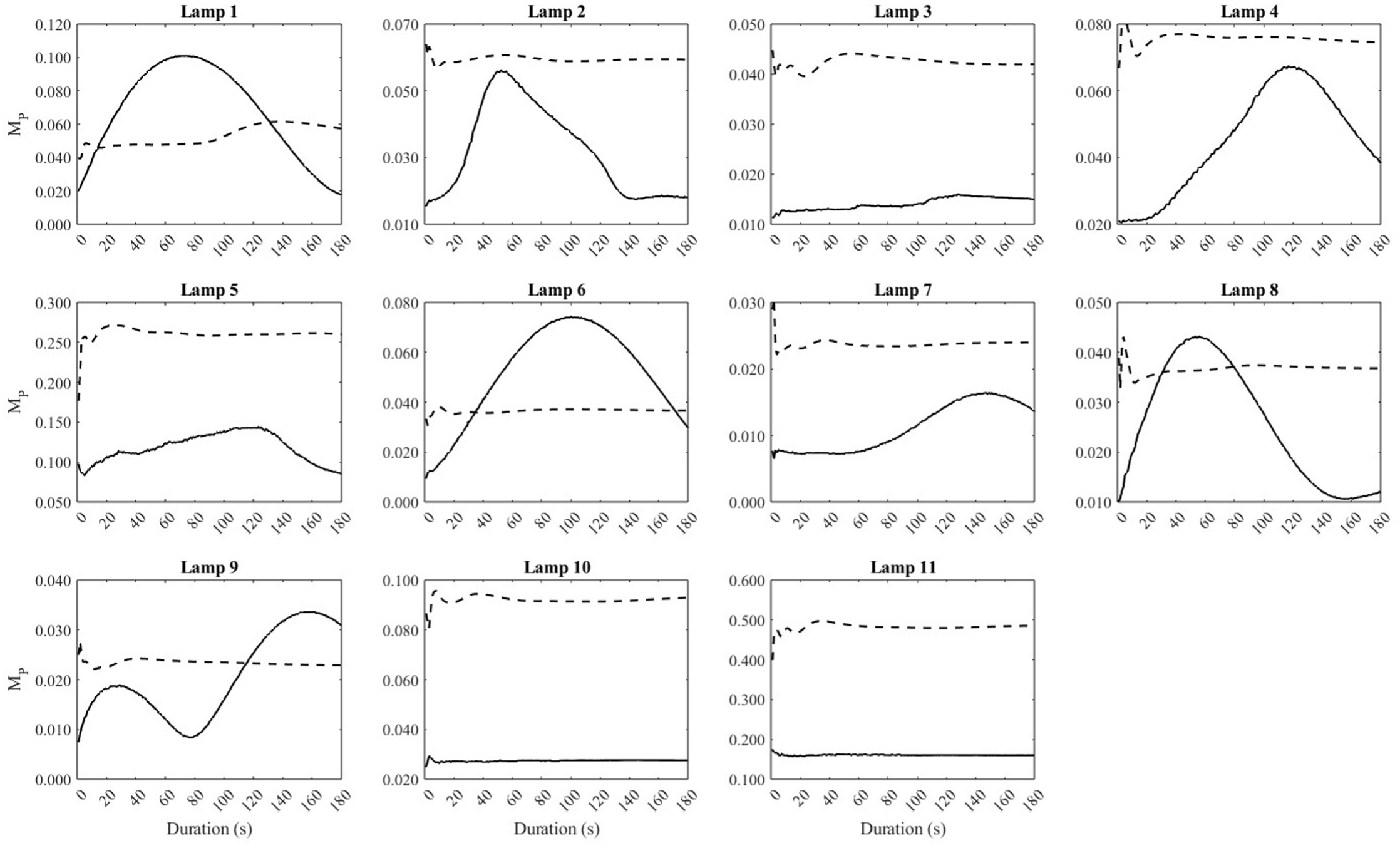
M _P values calculated for the waveforms of measurement durations varied from 1 s to 180 s (solid curve), and the corresponding revised metric, M_P,26, calculated using the revised method and recommended measurement conditions described in subsequent sections (dashed curve). Waveforms used for the calculations were measured with an anti-aliasing filter featuring a 1 kHz cut-off frequency and a 12 dB/octave roll-off, and were digitized at a sampling rate of 10 kHz.

The impact of starting phase of the waveforms on the M_P and the revised M_P,26 values was also investigated. The waveforms used for the M_P calculation were filtered at 1 kHz cut-off frequency and sampled at 50 kHz, and the waveforms for M_P,26 calculation were filtered at 1 kHz cut-off frequency and sampled at 10 kHz as recommended in the following sections. The measured filtered waveforms were cut into segments of the same waveform length (100 s) with varied starting sample points for calculating M_P. The total number of the sampling points within one cycle of each waveform is around 833 which can be obtained by dividing the duration of one cycle by the sampling time interval ((1/60 Hz)/(1/50 000 Hz)). The phase interval between the sampling points is around 0.432°. For calculating M_P,26, the waveforms were cut into segments of 6 s, which is the recommended duration for M_P,26 measurement. Calculating the M_P and M_P,26 values of waveform segments starting from each sample point of the first cycle gives M_P and M_P,26 as functions of starting phases, shown as solid and dashed lines in Figure 3. Relatively large variations in M_P values can be observed for many of the lamp waveforms, due to different starting phases. The revised M_P,26 values, measured at recommended conditions, show virtually no variation due to starting phases. These variations in M_P values for different measurement durations and starting phases are evidently due to spectral leakage, which is minimized by the revised calculation method of M_P,26, as described in the next section.

Figure 3

M _P values calculated for the measurement waveforms of starting phases varied from 1° to 360° (solid curve), and the corresponding revised metric, M_P,₂₆, calculated using the revised method and recommended measurement conditions described in subsequent sections (dashed curve). Waveforms used for the calculations were low-pass filtered with a 1 kHz cut-off frequency and a 12 dB/octave roll-off. For M_P calculations, the waveforms were sampled at 50 kHz over a duration of 100 s, whereas for M_P,₂₆ calculations, they were sampled at 10 kHz over a duration of 6 s

Similar reductions in measurement uncertainty were observed in simulations using waveforms with 100% modulation and M_P values well above the visual threshold of 1. Figure 4 shows an example of M_P variation for simulated sinusoidal waveforms modulated at 64.1 Hz and 64.9 Hz. The waveforms have a duration of 6 s and were sampled at 10 kHz as recommended in the following sections. The variation of M_P values (∼1.8 in absolute values of M_P) has been removed by using the revised calculation method. This indicates that the method is effective even when the simulated flicker is very strong and easily perceptible. This result is consistent with what was observed in measurements of a commercial lamp that had very low M_P values – i.e. very little flicker. Together, these findings demonstrate that the relative improvement in measurement uncertainty applies across a wide range of flicker levels, from barely perceptible to clearly visible.

Figure 4

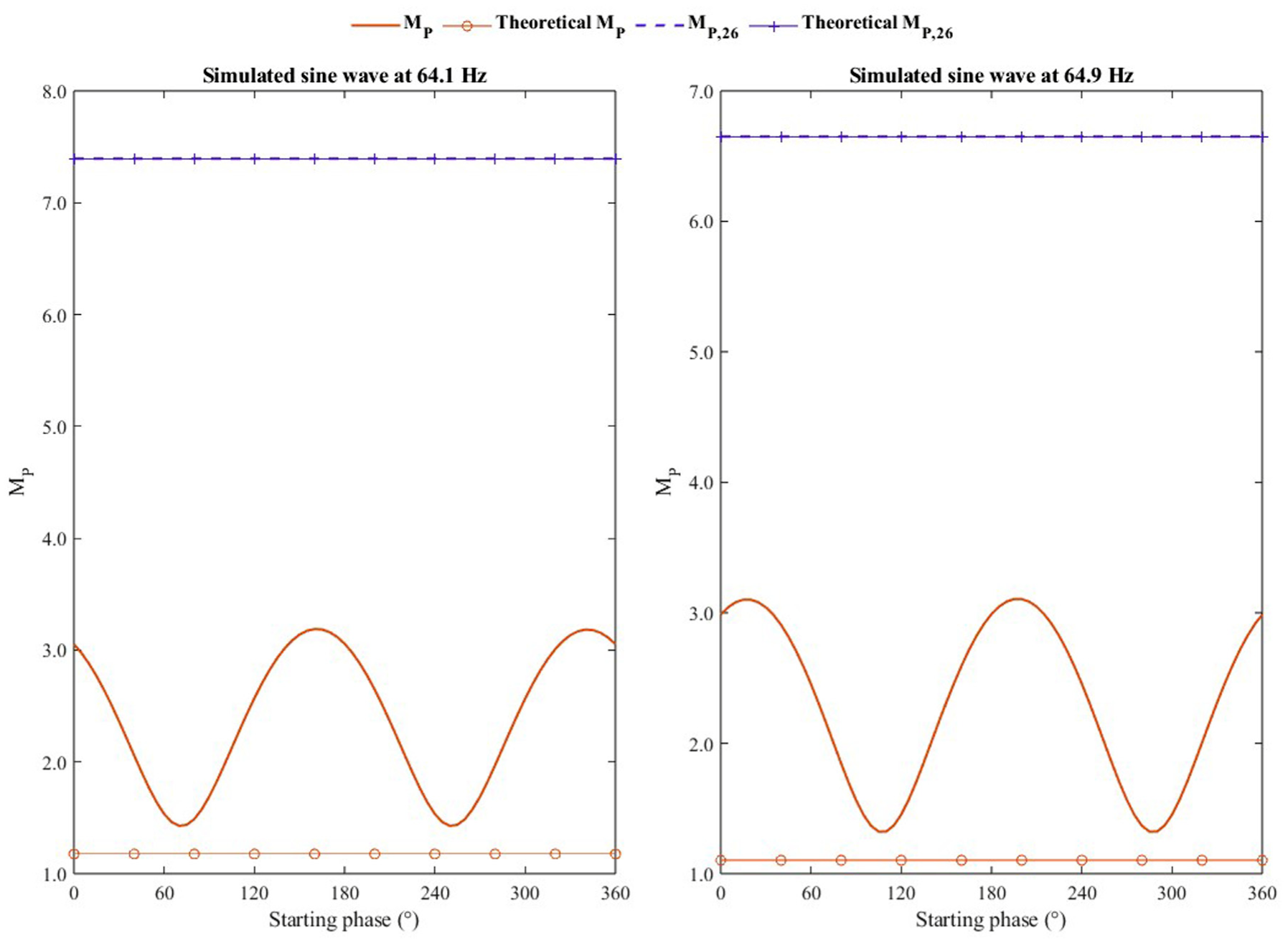
M _P values calculated for the simulated sine waveforms of starting phases varied from 1° to 360° (solid curve), and the corresponding revised metric, M_P,₂₆, calculated using the revised method and recommended measurement conditions described in subsequent sections (dashed curve). Theoretical M_P and M_P,₂₆ values derived directly from the sensitivity curves are also shown as markers at the 180° starting phase for visual comparison

Although the products shown in Figure 3 exhibit relatively low M_P values, products with higher $P_{\mathrm{st}}^{\mathrm{LM}}$ and M_P values (reaching up to 1.9) ²⁵ are available on the market in places other than Europe (e.g. Australia), based on data from the IEA SSL Annex platform. It is also important to note that flicker metrics are used not only for lamp products alone but also to combinations of lamps with dimmers or other devices, which can produce high M_P or $P_{\mathrm{st}}^{\mathrm{LM}}$ values.

3. Revised method of M_P calculation

3.1 Hann window

Spectral leakage is thought to be the cause of the substantial variation in M_P values for the same waveforms when resampled at different measurement durations and starting phases, and due to the varied amplitudes of the circular discontinuities. ²² This effect had not been explicitly considered in the original formulation of M_P, nor in similar metrics such as Perz et al.’s FVM, which also lacked the application of proper windowing techniques with window correction factors to mitigate spectral leakage. A windowing technique is often used to improve this spectral leakage issue in digital signal processing, as explained in Section 1. Illustrations of a rectangular window (a weighting of 1 everywhere, so no change to the originally sampled data), a Hann window and a flattop window are shown in Figure 5. This technique allows the two ends of the measured waveform signal to coincide in zero amplitude, resulting in a cyclical time-domain signal with no added discontinuities.

Figure 5

(a) Window functions and (b) their amplitude-normalized DFT spectra for a sine wave with a 30-Hz modulation frequency, sampled at 20 kHz

Several different types of window functions have been developed for digital signal processing, depending on the type of spectral information sought. For example, Figure 5 shows how different windowing techniques (rectangular, Hann and flattop) affect the calculated spectral content for a 30 Hz sinewave. A Hann (or Hanning) window is generally the best option in most cases, balancing spectral resolution (the width of the spectral peak) with reduced spectral leakage. The Hann window has a sinusoidal shape (see Figure 5), which reaches zero at both ends avoiding all cyclical discontinuity in the analysed signal.

To reduce the spectral leakage, a Hann window was added in the M_P calculation method before performing the FT. With the addition of the Hann window, the variation in M_P values due to the DFT spectral leakage has been largely reduced. Mantela et al. also pointed out the need for windowing in computing TLM metrics. ²⁶

3.2 Window effect correction factor

The added Hann window affects the DFT components of the waveforms in that it decreases the amplitude of the DFT peaks while broadening their bandwidths (see Figure 5). Therefore, if keeping the same perceptual sensitivity weighting function of M_P, the addition of the Hann window would result in a different DFT spectrum, and thus a different M_P value, termed M_P,H. This discrepancy between the M_P,H and the original M_P with its uniform window, which can also be considered as using a rectangular window, termed M_P,R, should be corrected as it does not reflect a difference in perception. The following steps were used to derive the correction factor for the window effect.

The window effect on M_P can be quantified by the ratio of the sum of the squared FT components of the Hann windowed waveform to the sum of the squared FT components of the rectangular windowed waveform. This ratio will be used to correct the effect of the Hann window so that values of the revised M_P have the same meaning as the original M_P values. For easier calculation, the summation of discrete FT frequency components is replaced by an integral of spectral density over frequency. As the use of the continuous formulation simplifies the mathematics with equivalent results, it will be used throughout the following mathematical derivations.

The Hann windowed M_P ( $M_{\mathrm{P},\mathrm{H}}$ ) and the original rectangular windowed M_P ( $M_{\mathrm{P},\mathrm{R}}$ ), can be equated by introducing a constant window correction factor, $c$ to scale the magnitude of the FT frequency components of the Hann windowed waveform. Therefore, the ratio between the corrected Hann windowed M_P ( $M_{\mathrm{P},\mathrm{H},\mathrm{c}}$ ) and the original rectangular windowed M_P ( $M_{\mathrm{P},\mathrm{R}}$ ) is 1, given as Equation (3). M_DTH,f is the modulation detection threshold value for each frequency f and A_f,_H and A_f,_R are the corresponding modulation amplitudes of the Hann windowed and rectangular windowed functions, respectively.

$$\frac{M_{\mathrm{P},\mathrm{H},\mathrm{c}}}{M_{\mathrm{P},\mathrm{R}}}=\frac{\sqrt{{\int }_{-\infty }^{\infty }{\left(\frac{A_{f,\mathrm{H}}}{c\times A_{0,\mathrm{H}}}\right)}^2\times \frac{1}{M_{\mathrm{DTH},f}^2}\mathrm{d}f}}{\sqrt{{\int }_{-\infty }^{\infty }{\left(\frac{A_{f,\mathrm{R}}}{A_{0,\mathrm{R}}}\right)}^2\times \frac{1}{M_{\mathrm{DTH},f}^2}\mathrm{d}f}}=1$$

(3)

In Equation (3), the DC components in the Hann windowed ( $A_{0,\mathrm{H}}$ ) and rectangular windowed ( $A_{0,\mathrm{R}}$ ) functions can be taken out of the integrals as constants. The DC amplitude of the Hann window function is 1/2, while that of the rectangular function is 1; these scale the DC components of A_R and A_H. The FT frequency components of the windowed temporal modulation waveform are obtained from the FT of the product of the temporal waveform ( $p\left(t\right)$ ) and the window function ( $w\left(t\right)$ ), where $\mathcal{F}$ represents the FT. By substituting the values of DC amplitudes, the centre ratio in Equation (3) is given by Equation (4).

$$\begin{array}{c}\multicolumn{1}{c}{\frac{M_{\mathrm{P},\mathrm{H},\mathrm{c}}}{M_{\mathrm{P},\mathrm{R}}}=\frac{A_{0,\mathrm{R}}}{A_{0,\mathrm{H}}}\times \frac{\sqrt{{\int }_{-\infty }^{\infty }{\left(\frac{A_{f,\mathrm{H}}}{c\times M_{\mathrm{DTH},f}}\right)}^2\mathrm{d}f}}{\sqrt{{\int }_{-\infty }^{\infty }{\left(\frac{A_{f,\mathrm{R}}}{M_{\mathrm{DTH},f}}\right)}^2\mathrm{d}f}}}\\ \multicolumn{1}{c}{=2\times \frac{\sqrt{{\int }_{-\infty }^{\infty }\frac{{\mathcal{F}}^2(p\left(t\right)\times w_{\mathrm{H}}\left(t\right))}{c^2\times M_{\mathrm{DTH},f}^2}\mathrm{d}f}}{\sqrt{{\int }_{-\infty }^{\infty }\frac{{\mathcal{F}}^2(p\left(t\right)\times w_{\mathrm{R}}\left(t\right))}{M_{\mathrm{DTH},f}^2}\mathrm{d}f}}}\end{array}$$

(4)

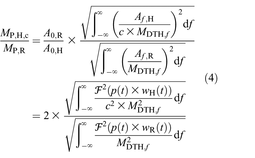
Based on the Convolution Theorem, the FT of a convolution of two functions is the pointwise product of their FT. Therefore, the FT of the product of the temporal wave ( $p\left(t\right)$ ) and the window function ( $w\left(t\right)$ ) in Equation (4) can be converted to the convolution of their FT spectra ( $P_f$ , $W_f$ ) as shown in Equation (5).

$$\begin{array}{c}\multicolumn{1}{c}{2\times \frac{\sqrt{{\int }_{-\infty }^{\infty }\frac{{(P_f\otimes W_{f,\mathrm{H}})}^2}{c^2\times M_{\mathrm{DTH},f}^2}\mathrm{d}f}}{\sqrt{{\int }_{-\infty }^{\infty }\frac{{(P_f\otimes W_{f,\mathrm{R}})}^2}{M_{\mathrm{DTH},f}^2}\mathrm{d}f}}=}\\ \multicolumn{1}{c}{2\times \frac{\sqrt{{\int }_{-\infty }^{\infty }\frac{1}{c^2\times M_{\mathrm{DTH},f}^2}{[\int W_{\mathrm{H}}(f-\xi )P\left(\xi \right)\mathrm{d}\xi ]}^2\mathrm{d}f}}{\sqrt{{\int }_{-\infty }^{\infty }\frac{1}{M_{\mathrm{DTH},f}^2}{[\int W_{\mathrm{R}}(f-\xi )P\left(\xi \right)\mathrm{d}\xi ]}^2\mathrm{d}f}}}\end{array}$$

(5)

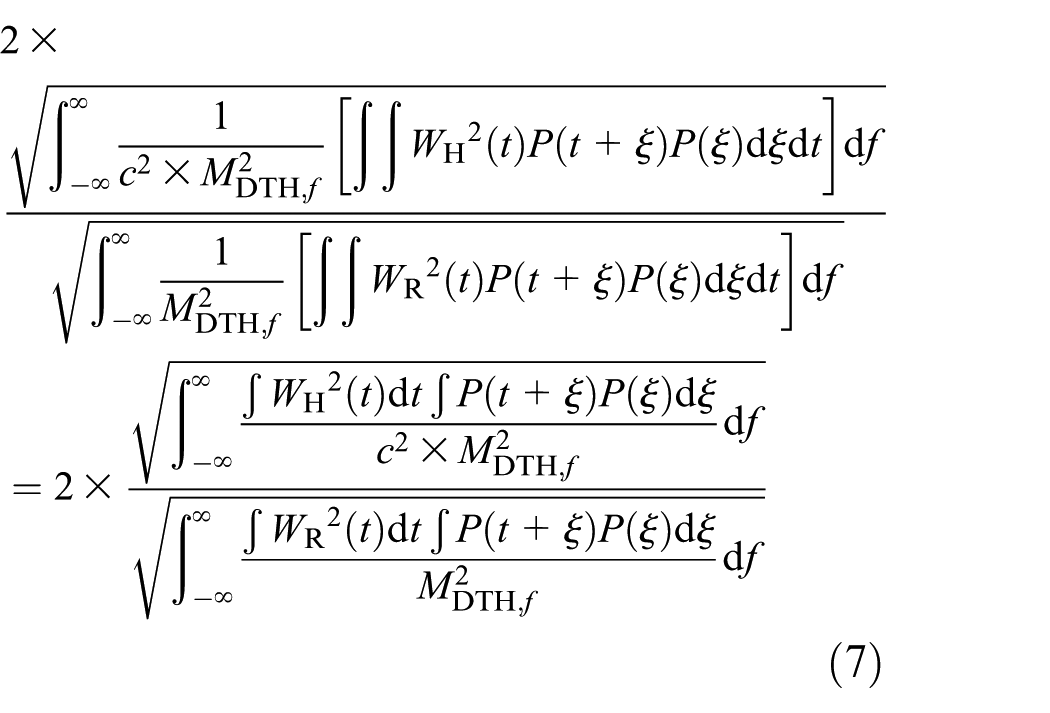
From Fubini’s Theorem, ²⁷ a double integral can be computed by using an iterated integral, the square of the integral in the numerator of Equation (5) is therefore given as shown in Equation (6).

$$\begin{array}{c}\multicolumn{1}{c}{{[\int W_{\mathrm{H}}(f-\xi )P\left(\xi \right)\mathrm{d}\xi ]}^2}\\ \multicolumn{1}{c}{\int =W_{\mathrm{H}}(f-\xi )P\left(\xi \right)\mathrm{d}\xi \int W_{\mathrm{H}}(\xi -f)P\left(f\right)\mathrm{d}f}\\ \multicolumn{1}{c}{=\int \int W_{\mathrm{H}}(f-\xi )W_{\mathrm{H}}(\xi -f)P\left(f\right)P\left(\xi \right)\mathrm{d}\xi \mathrm{d}f}\\ \multicolumn{1}{c}{=\int \int W_{\mathrm{H}}\left(t\right)W_{\mathrm{H}}(-t)P(t+\xi )P\left(\xi \right)\mathrm{d}\xi \mathrm{d}t}\end{array}$$

(6)

Equation (6) can be substituted into the numerator and denominator of Equation (5). As the FT spectrum of the window is left–right symmetric on the frequency axis, the expression in Equation (5) can be rewritten as in Equation (7).

$$\begin{array}{c}\multicolumn{1}{c}{2\times }\\ \multicolumn{1}{c}{\frac{\sqrt{{\int }_{-\infty }^{\infty }\frac{1}{c^2\times M_{\mathrm{DTH},f}^2}[\int {W_{\mathrm{H}}}^2\left(t\right)P(t+\xi )P\left(\xi \right)\mathrm{d}\xi \mathrm{d}t]\mathrm{d}f}}{\sqrt{{\int }_{-\infty }^{\infty }\frac{1}{M_{\mathrm{DTH},f}^2}[\int \int {W_{\mathrm{R}}}^2\left(t\right)P(t+\xi )P\left(\xi \right)\mathrm{d}\xi \mathrm{d}t]\mathrm{d}f}}}\\ \multicolumn{1}{c}{=2\times \frac{\sqrt{{\int }_{-\infty }^{\infty }\frac{\int {W_{\mathrm{H}}}^2\left(t\right)\mathrm{d}t\int P(t+\xi )P\left(\xi \right)\mathrm{d}\xi }{c^2\times M_{\mathrm{DTH},f}^2}\mathrm{d}f}}{\sqrt{{\int }_{-\infty }^{\infty }\frac{\int {W_{\mathrm{R}}}^2\left(t\right)\mathrm{d}t\int P(t+\xi )P\left(\xi \right)\mathrm{d}\xi }{M_{\mathrm{DTH},f}^2}\mathrm{d}f}}}\end{array}$$

(7)

From Equation (7), it is clear that if this is to be equal to 1, $c$ must be as given in Equation (8).

$$c=2\times \sqrt{\frac{\int {W_{\mathrm{H}}}^2\left(t\right)\mathrm{dt}}{\int {W_{\mathrm{R}}}^2\left(t\right)\mathrm{dt}}}$$

(8)

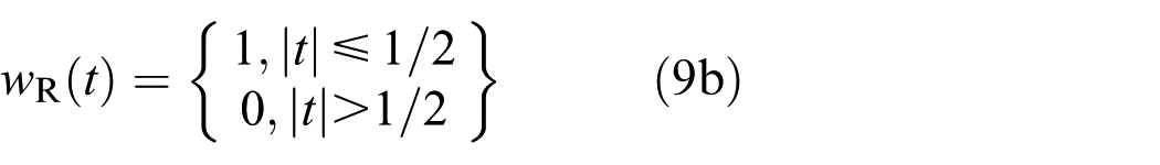
For a unit length window, the Hann window and rectangular window functions in the time domain can be mathematically described as shown in Equations (9a) and (9b).

$$w_{\mathrm{H}}\left(t\right)=\left\{\begin{array}{c}\frac{1}{2}+\frac{1}{2}\cos \left(2\pi t\right),\left|t\right|\le 1/2\hfill \\ \multicolumn{1}{c}{0,\left|t\right|>1/2}\end{array}\right\}$$

(9a)

$$w_{\mathrm{R}}\left(t\right)=\left\{\begin{array}{c}1,\left|t\right|\le 1/2\hfill \\ \multicolumn{1}{c}{0,\left|t\right|>1/2}\end{array}\right\}$$

(9b)

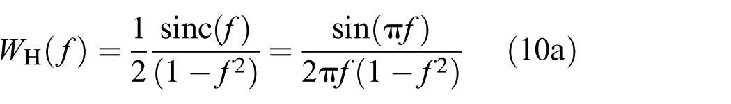
The FT frequency response of a unit length Hann window and a rectangular window are as given in Equations (10a) and (10b).

$$W_{\mathrm{H}}\left(f\right)=\frac{1}{2}\frac{\mathrm{sinc}(f)}{(1-f^2)}=\frac{\sin (\pi f)}{2\pi f(1-f^2)}$$

(10a)

$$W_{\mathrm{R}}\left(f\right)=\mathrm{sinc}(f)=\frac{\sin (\pi f)}{\pi f}$$

(10b)

By substituting the FT spectra of the window functions (Equations (10a) and (10b)) and eliminating the identical parts in the numerator and denominator in Equation (8), $c$ can be calculated as in Equation (11).

$$\begin{array}{c}\multicolumn{1}{c}{c=2\times \sqrt{\frac{{\int }_{-\infty }^{\infty }{\left(\frac{\sin \left(\pi f\right)}{2\pi f(1-f^2)}\right)}^2\mathrm{d}f}{{\int }_{-\infty }^{\infty }{\left(\frac{\sin \left(\pi f\right)}{\pi f}\right)}^2\mathrm{d}f}}}\\ \multicolumn{1}{c}{=2\times \sqrt{\frac{3}{8}}\cong 1.225}\end{array}$$

(11)

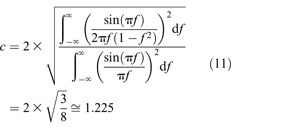
Using the same method as described above for other window functions leads to different correction factors. For example, the correction factor for a Bartlett (triangular) window is approximately 1.155, and for a flattop window is approximately 1.942.

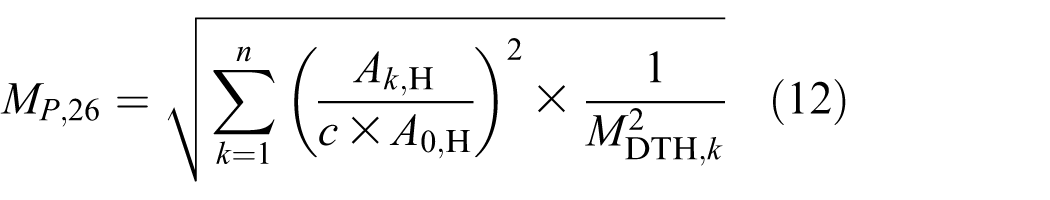
The Hann window corrected form $M_{\mathrm{P},\mathrm{H},\mathrm{c}}$ , denoted as M_P,26, can be calculated using Equation (12), which incorporates the window correction factor c.

$$M_{P,26}=\sqrt{\sum _{k=1}^n{\left(\frac{A_{k,\mathrm{H}}}{c\times A_{0,\mathrm{H}}}\right)}^2\times \frac{1}{M_{\mathrm{DTH},k}^2}}$$

(12)

As shown in Figure 6, the M_P variations due to spectral leakage are significantly reduced after adding the Hann window and its correction factor. The sensitivity curve of the M_P metric derived from Bodington et al.’s experiment starts with a relatively high value at 5 Hz modulation frequency and ends with a small but non-zero value at 65 Hz. At modulation frequencies below 5 Hz or above 65 Hz, the weighting values are all set to zero. As a result, the weighting value changes abruptly at 5 Hz and, to a lesser extent at 65 Hz. However, there is often an uncertainty in the dominant frequency of a DFT spectrum of measured waveforms, due to different sampling durations and the phase of the waveform when sampling starts. This uncertainty is especially high for short duration waveforms due to low frequency resolution in the resulting DFT spectrum. When this uncertainty in the dominant frequency occurs at the end of the weighting function’s frequency range (e.g. 5 Hz), it results in a large variability in the M_P values, from values near zero to several hundred, depending on the waveform. Therefore, the abrupt change in the weighting function at 5 Hz may result in a potential problem for the evaluation of the direct flicker effect of the TLM using the M_P metric without a method to prevent this from happening. Fortunately, the use of the Hann window greatly reduces the variations in M_P due to the metric’s sensitivity cut-offs at 5 Hz and 65 Hz. Spectral broadening will result in some of the actual spectral content less than 5 Hz being transferred (leaked) to frequencies greater than 5 Hz and inflating the metric. Likewise, some spectral content above 5 Hz is assigned to frequencies less than 5 Hz and does not contribute to M_P. The combined effect is a smooth transition from cut-off to cut-on frequencies. The benefit of using the Hann window is that this leakage is much more limited across frequencies and much less in magnitude for different sampling phases and durations than with a rectangular window. Figure 6 compares M_P with and without Hann windowing by plotting the range of M_P values obtained for sine waves sampled over a range of phases (100 random phases) from 0 to 2π. The Hann-windowed method reduces M_P variation at each frequency to negligible amounts and produces a less abrupt transition at the 5 Hz cut-off frequency. This less abrupt transition at 5 Hz with negligible variations due to starting phase is preferable to the much larger and variable spectral leakage of the rectangular window that extends farther in frequency from the 5 Hz cut-off.

Figure 6

M _P with and without Hann window as a function of modulation frequency for 2-s sine waveforms at 100% modulation sampled over a range of starting phases from 0 to 2π. The median and interquartile range of M_P values at each frequency for different waveform starting phases are shown as solid lines and shaded regions (red for without Hann window, blue for with Hann window). The interquartile range for the M_P with Hann window is indistinguishable from the line

4. Modifications in the sensitivity weighting function

The perceptual sensitivity weighting function in the original M_P calculation covers the modulation frequencies from 5 Hz to 65 Hz. Furthermore, the original sensitivity curve of the M_P metric is derived under an experimental condition simulating an individual lamp in a small indoor environment, which may underestimate the direct flicker effect in application scenarios with higher light levels and high correlated colour temperature (CCT), where the direct flicker effect tends to be more severe and harmful to health. Therefore, another sensitivity curve from the study of Perz et al., ²¹ obtained under high CCT (6500 K) and high luminance (209 cd m⁻²) conditions was adopted because it represents viewing conditions that heighten direct flicker sensitivity and extends the sensitivity range to 80 Hz. This sensitivity curve is incorporated in the revised M_P for characterization of the direct flicker effect in a wider range of applications. The sensitivity curve was mathematically derived following the same procedure described in Perz’s publication. ²¹ In their study, flicker visibility thresholds were first averaged across participants. These mean threshold values were then converted into sensitivity values by taking their reciprocals. The mean sensitivities, expressed on a logarithmic scale as a function of log frequency, were subsequently interpolated using a shape-preserving piecewise cubic interpolation to generate the TCSF.

A comparison of the two sensitivity curves is shown in Figure 7. According to the IEEE Standard 1789 and other literature reviews, flicker causing health issues typically occurs in the modulation frequency range of 3 Hz to 70 Hz.^16,17 Accordingly, the revised M_P,26 calculation method also incorporates this updated sensitivity weighting curve from 3 Hz (indicated as dotted line in Figure 7) to 80 Hz.

Figure 7

Sensitivity (1/visibility detection threshold) curves for sinusoidal waveforms as a function of frequency derived from the study of Bodington et al., ¹³ and the study of Perz et al. ²¹

5. Recommended measurement conditions for M_P,26 calculation

We have evaluated the variation of M_P,26 caused by varied spectral leakage due to different starting phases, based on simulated sinusoidal and square waves. An example of the M_P,26 variation at modulation frequencies below 10 Hz at 2 s measurement duration is shown in Figure 8, for sinusoidal and square waves with 100% percent flicker. The median values and interquartile range of M_P,26 are indicated. The variation of M_P,26 is negligible for sinusoidal waves, but more noticeable for square waves, especially at modulation frequencies below 3 Hz, where the transition in the sensitivity curve is much sharper. (Note that for square waves, M_P,26 does not quickly decrease to zero below the 3 Hz cut-off because of the higher frequency harmonics present in square waves.) M_P,26 at low modulation frequencies varies more with short measurement durations (e.g. 2 s), where the lower DFT spectral resolution results in higher spectral uncertainty at the dominant frequency. Increasing the measurement duration (e.g. 5 s) would reduce the spectral uncertainty and the M_P,26 variations, as shown in Figure 8c. In practice, a duration of 5 s will result in negligible errors.

Figure 8

M _P,26 as a function of frequency for sine waves (a, duration 2 s) and square waves (b, duration 2 s; c, duration 5 s) at 100% modulation, sampled over a range of starting phases from 0 to 2π. The median and interquartile range of M_P,26 values at each frequency across different starting phases are shown as solid lines and shaded regions (red for sine waves, blue for square waves). For the sine wave and the 5 s square wave, the shaded interquartile ranges are indistinguishable from the lines

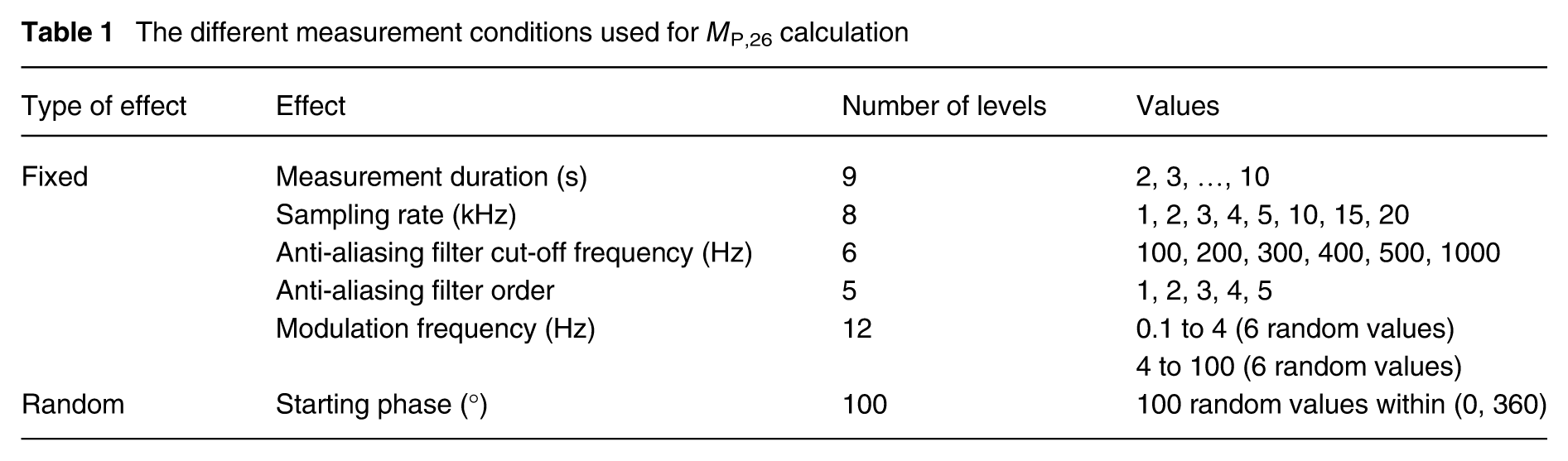
Therefore, it is crucial to evaluate and recommend the minimum measurement duration for accurate M_P,26 calculation. Besides, the sampling rate might be influential on calculated M_P,26 when an anti-aliasing filter is applied in practical measurements. The effects of measurement duration, sampling rate and anti-aliasing filter setting (digital anti-aliasing filters with different cut-off frequencies and filter orders) on M_P,26 variation due to different starting phases were investigated at varied modulation frequency below and above 3 Hz, respectively, using simulated square waveforms with random noise added. The signal noise was simulated based on the noise of the dark current measured at the NIST photometry lab during the IC 2023. The conditions are shown numerically in Table 1.

Table 1

The different measurement conditions used for M_P,26 calculation

Type of effect	Effect	Number of levels	Values
Fixed	Measurement duration (s)	9	2, 3, …, 10
	Sampling rate (kHz)	8	1, 2, 3, 4, 5, 10, 15, 20
	Anti-aliasing filter cut-off frequency (Hz)	6	100, 200, 300, 400, 500, 1000
	Anti-aliasing filter order	5	1, 2, 3, 4, 5
	Modulation frequency (Hz)	12	0.1 to 4 (6 random values) 4 to 100 (6 random values)
Random	Starting phase (°)	100	100 random values within (0, 360)

Since the sampling rate is required to be higher than twice the Nyquist frequency of the anti-aliasing filter, only sampling rates complying with the Nyquist criterion were used to configure the measurement conditions for the M_P,26 calculations. The M_P,26 values for 100 random starting phases were calculated for each combined measurement condition. A total of 1 296 000 simulated waveforms with varying conditions and random starting phases were generated for modulation frequencies both below and above 4 Hz. The M_P,26 results were statistically analysed in RStudio using a generalized linear mixed-effects model (R function glmer). ²⁸ The model accommodated the unbalanced design, which included differing numbers of M_P,26 observations across conditions. Residual diagnostics were conducted using the DHARMa package, ²⁹ to verify the model’s validity and robustness. The statistical results are indicated in Table 2. According to the analysis of variance (ANOVA) for the general linear mixed-effect model, the measurement duration, anti-aliasing filter setting (cut-off frequency, filter order and their interaction) and modulation frequency have statistically significant impact on M_P,26 variation with a p-value of <0.01.

Table 2

ANOVA table (Type III Wald chi-square tests) for the impact of different measurement conditions on the M_P,26 variation at modulation frequencies below 4 Hz (significant impact factors are in italic)

Impact factors and interactions	Degree of freedom	p Value
Measurement duration	8	<0.001
Sampling rate	7	<0.001
Anti-aliasing filter cut-off frequency	5	0.0040
Anti-aliasing filter order	4	0.8214
Modulation frequency	5	1.0000
Interaction between sampling rate and filter cut-off frequency	32	0.0238
Interaction between sampling rate and filter order	27	1.0000
Interaction between filter cut-off frequency and filter order	20	<0.001
Interactions between sampling rate, filter cut-off frequency and filter order	95	1.0000

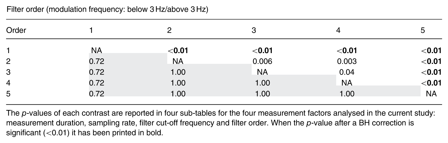
To find which measurement settings (duration, filter setting) result in significantly different M_P,26 variations, pairwise comparisons between factor levels (different durations, filter cut-off frequencies, filter orders, etc.) based on the statistical model output were conducted using the R-function ‘emmeans’ in ‘emmeans’ library. ³⁰ The pairwise comparison results were confirmed based on the raw data by the pairwise t-test using the R-function ‘pairwise.t.test’ with Benjamini and Hochberg (‘BH’) testing corrections. ³¹ The ‘BH’ methods control the false discovery rate, the expected proportion of false discoveries amongst the rejected hypotheses. ³² The numerical details of corrected p-values for pairwise comparison of duration levels are included in Table A2. The results show that for modulation frequencies below 3 Hz, measurement durations of 5 s or shorter yield a significantly larger M_P,26 variation compared to longer measurement durations. Furthermore, for measurement durations longer than 6 s, the M_P,26 variation is no longer (statistically) significantly different. Additionally, a measurement duration of 5 s results in practically negligible errors. Therefore, we recommend a minimum measurement duration of 5 s for more accurate M_P,26 calculations at modulation frequencies below 3 Hz. No statistically significant difference was found between the different filter settings based on the results of pairwise comparison analysis after the BH correction (though the interaction between the cut-off frequency and filter order was found significant from the ANOVA table), which is reasonable as the evaluated modulation frequencies (≤3 Hz) are very low compared to the filter cut-off frequencies.

The same statistical analysis was performed for waveforms with modulation frequencies above 3 Hz (from 3 Hz to 100 Hz), where the M_P,26 sensitivity curve changes smoothly leading to smaller M_P,26 variation. The significant impact factors found for modulation frequency below 3 Hz were also found significant above 3 Hz. In addition, the sampling rate was found to be an additional significant impact factor for modulation frequency above 3 Hz. With higher frequency components present in the testing waveforms, the sampling rate becomes critical for successful anti-aliasing.

The pairwise comparison results for modulation frequency above 3 Hz are also shown in Table A2. Based on the pairwise comparison analysis, at a sampling rate of 1 kHz, the M_P,26 variation is significantly different from the higher sampling rates. The pairwise comparison result also indicates significant difference in M_P,26 measured at 1 s compared to other durations. These results lead us to recommend a minimum measurement duration of 5 s and a sampling rate of at least 2 kHz for M_P,26 measurements. Regarding filter settings, a significant difference in M_P,26 variation was observed between filters with cut-off frequencies below and above 400 Hz at modulation frequencies above 3 Hz. Therefore, we recommend using a cut-off frequency of ≥400 Hz when the filter’s cut-off is not sufficiently sharp. A filter order of at least 2 is also recommended, as first-order filters produced M_P,26 results that differed significantly from those obtained with the other four tested filter orders, while no significant differences were found among orders 2 and higher. A recent study by Li et al. ¹² has shown that the sampling rate of a first-order anti-aliasing filter may need more than twice the Nyquist frequency depending on the waveform. The current M_P,26 results obtained for the first-order anti-aliasing filter may therefore be different from those for other filter orders due to the same reason. A summary of recommended measurement conditions for the M_P,26 calculation is indicated in Table 3.

Table 3

Recommendation of measurement conditions for M_P,26 calculation

Measurement condition	Recommended value
Measurement duration	≥5 s
Sampling rate	≥2 kHz
Anti-aliasing filter cut-off frequency	≥400 Hz
Anti-aliasing filter order	≥2

Taking the 100% modulated square wave as an example, the M_P values are calculated both with the original method and the revised method for modulation frequencies between 3 Hz and 100 Hz with an interval of 0.05 Hz. The uncertainty in M_P is estimated by the standard deviation at each modulation frequency. Comparing the M_P calculated with the original method using 2 s duration and 1 kHz sampling rate, with the revised M_P,26 using the proposed measurement conditions (5 s measurement duration, 2 kHz sampling rate, 400 Hz cut-off frequency and second order anti-aliasing filter), the average uncertainties have been reduced to 5% of the original for modulation frequency between 3 Hz and 100 Hz. The average standard deviation, normalized to the mean calculated M_P, was reduced from 38.42% to 0.29%. Additionally, the average absolute uncertainty – initially 5.15 (well above the metric’s visibility threshold of 1) – was reduced to 0.09. The improved reproducibility of M_P,26 for typical light sources is illustrated in Figures 2 and 3.

5. Conclusions

In the current study, the light waveforms of 11 typical commercial lamps including 10 LED lamps and 1 CFL were measured. Substantial variations in the original M_P values (defined in the ASSIST document) ⁷ for some types of waveforms were found when using different durations and starting phases, and it was discovered that this was due to the DFT spectral leakage caused by finite duration waveform sampling. The M_P variation caused by spectral leakage was greatly improved by adding a Hann window. To maintain the perceptual relevance of the revised M_P, a window correction factor was added to account for the window’s effect on integrated spectral power. To broaden the scope of application of the M_P metric, the sensitivity weighting function in the M_P calculation was replaced by the one derived from the experimental data of Perz et al. in 2017, covering a frequency range of 3 Hz to 80 Hz. Specific waveform measurement conditions, including measurement duration, sampling rate and the anti-aliasing filter settings, were recommended based on an extensive statistical analysis of M_P,26 variation due to these effects. A linear mixed-effects model was fitted to the M_P,26 results as a function of different measurement effects (duration, sampling rate, filter cut-off frequency and filter order). A pairwise comparison between different levels in each measurement effect was conducted. A measurement duration of ≥5 s, sampling rate of ≥2 kHz, anti-aliasing filter cut-off frequency of ≥400 Hz and filter order ≥2 are recommended for accurate measurement and calculation of the revised M_P,26. With M_P,26 and the recommended measurement conditions, the average absolute uncertainties for measurement of the sample of 11 commercial lamps have been reduced to less than 5% of the original (from 5.15 to 0.09) for modulation frequency above 3 Hz. Similar percentage reductions in uncertainty were obtained for simulated waveforms having 100% modulation and M_P values much higher than the visual threshold of 1, thereby demonstrating that the relative improvement in measurement uncertainty seen in the commercial lamp sample exhibiting very low M_P values would also occur for lamps having perceptually high amounts of flicker. This study proposed an approach with ‘window + correction factor for integrated spectral power’ to be used in the frequency-domain TLA metrics without losing the perceptual correlation, and a novel statistical analysis using a linear mixed-effects model for comparing the different measurement conditions for metric calculation, providing a reference for the recommendations in regulations and standards for direct flicker evaluation in practical measurements. The MATLAB code for the M_P,26 is provided as Supplemental Material with this paper, and will also be made publicly available in the revision of ASSIST document when it is published. The perceptual threshold of the revised M_P,26 is planned to be validated through human visual experiments in future studies.

Supplemental Material

sj-docx-1-lrt-10.1177_14771535261435634 – Supplemental material for Revision of MP calculation method for flicker measurement

Supplemental material, sj-docx-1-lrt-10.1177_14771535261435634 for Revision of MP calculation method for flicker measurement by J Li, A Bierman and Y Ohno in Lighting Research & Technology