Critical review of the daylight glare probability and proposal for modification for improved evaluation of small glare sources

Abstract

EN 17037 defines essential properties of daylight in buildings: daylight provision, view out, sunlight exposure and glare protection. For assessing glare, the standard proposes the daylight glare probability (DGP) metric. A look at the formula reveals the following problem: since the luminance is included quadratically, but the solid angle only linearly, small but bright glare sources (e.g. the sun) are rated highly. This must be questioned if the glare stimulus can no longer be distinguished from larger stimuli causing equal vertical illuminance at the eye, especially in the peripheral visual field. For the unified glare rating for artificial lighting, this is avoided by limiting the minimum solid angle of the glare source. There is nothing comparable for the DGP. We present a simulation study on how the DGP changes with the bidirectional scattering distribution function resolution for complex fenestration systems or with rendering the sun at its real size. We performed subject experiments on the discriminability of small light stimuli in the periphery in a laboratory setup. Based on the findings, we propose adjusting the DGP by limiting the minimum glare source solid angle depending on its position in the field of view. We conclude with an evaluation of the simulation results with the modified metric daylight glare metric (DGM) and point out open issues that still need to be investigated.

1. Introduction

1.1 Motivation

Numerous studies and investigations have demonstrated the benefits of good daylighting in buildings. As Knoop et al. ¹ comprehensively summarized, daylight not only has a significant positive influence on the visual system, but also on the non-visual system. The International Energy Agency (IEA) emphasizes in a position paper ² that daylight is not only the preferred light source for humans, but also has significant influence on the energy demand in buildings for lighting, heating and cooling and can be regarded as regenerative energy source. Daylight in buildings must be planned accordingly in order to make the most of energy savings, health and well-being as well as visual comfort. Standards help to comply with the boundary conditions.

European standard EN 17037 Daylight in Buildings ³ was the first daylighting standard to come into force at European level. It defines the essential properties of daylighting in buildings in four categories: daylight provision, assessment for view out, exposure to sunlight and protection from glare. Two methods are proposed in the standard for evaluating daylight glare: a simplified procedure referring to EN 14500 ⁴ and EN 14501 ⁵ can be used for non-scattering glazing with low or variable transmittance, for textile screens or for systems that are opaque when closed. The general method, however, is that the time-resolved probability of occurrence of glare from daylight is determined using the daylight glare probability (DGP) metric. ⁶ This method must therefore be used in particular when daylighting or glare/solar protection systems are used (so-called complex fenestration systems, CFS), which are usually described and represented in simulations by their bidirectional scattering distribution function (BSDF).^7,8

DGP contains both, a saturation term and a contrast term, and both must be calculated with high accuracy. The vertical illuminance for the saturation term can well be simulated using low-resolution BSDFs (e.g. based on the Klems discretization^9,10). The contrast term, however, requires the accurate determination of the luminance and the corresponding solid angle of the glare source(s). For daylight, this is particularly relevant for the sun with its small solid angle (opening angle about 2 × 0.26°) and its high luminance (in the range of 1e9 cd m⁻²). To describe scattering or (partial) transmission of the sun through BSDFs in daylight simulations, several methods have been developed. Variable resolution BSDFs ¹¹ allow to reduce the solid angle covered by a single BSDF patch, or the ‘peak extraction (PE)’ algorithm ¹² allows to extract a direct-through component for the sun at its real size. These methods have also already been validated, and it has been proven that simulation and measurements lead to comparable results. ¹³

A look at the formula of the DGP reveals the problem here: since the luminance is included in the formula quadratically, but the solid angle only linearly, very small and very bright glare sources are rated highly. However, this must be questioned if the glare stimulus can no longer be distinguished from larger and less bright sources, especially in the peripheral visual field. For the unified glare rating (UGR), ¹⁴ which is used for glare evaluation of artificial lighting systems, this is avoided by limiting the allowed solid angle of the glare source. However, there is nothing comparable in EN 17037 for the DGP.

Against this background, we investigated how the DGP value – at constant vertical illuminance at the eye – changes with the used BSDF resolution or the use of the PE method. Based on subject experiments on the discriminability of glare stimuli in the peripheral visual field, we have developed an extension of the DGP metric that can be used to solve the problem.

1.2 Daylight glare probability

DGP was introduced by Wienold and Christoffersen ⁶ in 2006 and has since established itself as the standard metric for the assessment of glare caused by daylight. In a cross-validation based on various datasets from different research groups, in 2019 Wienold et al. ¹⁵ also showed that the DGP is the most robust in a comparison of all daylight glare metrics considered and best describes the glare perception of test participants. Initially used mainly in academia, DGP was gradually also adopted by planning offices. With the provision of the evalglare tool ¹⁶ for determining the DGP, the metric could be used by practitioners directly in Radiance ¹⁷ or via software based on it (e.g. the widely used Rhinoceros 3D plugins “Honeybee” from Ladybug Tools LLC and “ClimateStudio” from Solemma LLC).

In the meantime, the metric has also found its way into standardization and is therefore an important point of reference in practice. The European standard for daylight in buildings, EN 17037, ³ which was first published in 2018, includes the DGP as the method for assessing daylight glare. Even the simplified method that can be used for glazing with low transmittance or for textile screens refers to EN 14501, ⁵ where again the DGP is used to classify the systems. At the same time, the standard also points out that there are shortcomings to the method. One of these is that the DGP cannot be applied in situations where vertical illuminance is not a good indicator of the daylight glare sensation.

This can for example occur in office environments if a sun shading or glare protection device is installed that has low transmission, but still leads to high contrast scenarios. A typical example would be a textile glare protection system with some openness fraction (i.e. small holes between weave). In such setups, the primary glare source is the sun disc, which covers a tiny solid angle (about 2 × 0.26° aperture angle) but is extremely bright (luminance in the order of 1e9 cd m⁻², possibly only reduced through the glazing transmittance).

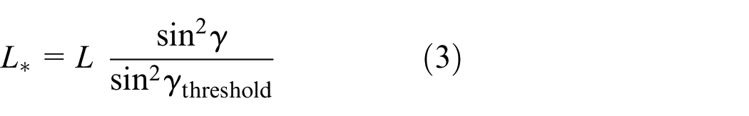
Looking at the DGP formula (Equation (1)) as given in the standard, one can see that in the contrast term (the sum of all glare sources) the luminance of the glare source is quadratic, while the solid angle is linear:

$$\begin{array}{cc}\multicolumn{1}{c}{\mathrm{DGP}=}& 5.87\times {10}^{-5}{E}_v+9.18\times {10}^{-2}\hfill \\ \multicolumn{1}{c}{}& \log (1+\sum _i\frac{L_{s,i}^2{\omega }_{s,i}}{E_v^{1.87}{P}_i^2})+0.16\hfill \end{array}$$

(1)

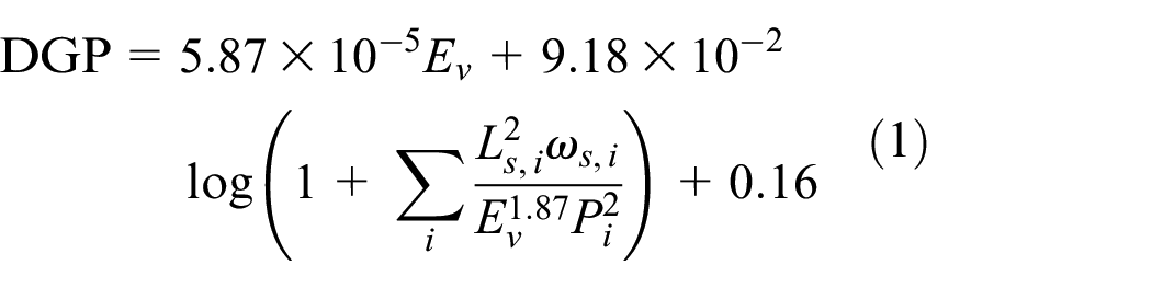
where $E_v(\mathrm{lx})$ is the vertical illuminance, $L_{s,i}^2(\mathrm{cd}{\mathrm{m}}^{-2})$ is the luminance of glare source i, ${\omega }_{s,i}(\mathrm{sr})$ is the solid angle of glare source i and $P_i$ is the position index for glare source i.

This is also consistent with other contrast-based glare metrics (e.g. UGR). For UGR, however, a lower limit is set for the size of the glare source in order to maintain the validity of the formula. ¹⁴ This limit is specified as 0.0003 sr, which corresponds to a cone with an opening angle of 2 × 0.56°, that is, approximately five times the solid angle of the sun. The question therefore arises as to whether a comparable lower limit is also required for the DGP metric.

The topic of glare source size is particularly important when evaluating visual comfort for daylighting or glare/sun protection systems. In simulation, CFS are usually described by their BSDF which is provided in tabulated, that is, discretized format. In the most common formats, the resolution of the data corresponds 2 × 6.7° for Klems, 2 × 2.5 to 7.5° for IEA T21 and 2 × 2.53°, 2 × 1.27° or 2 × 0.63° for Tensor Tree with k = 5, 6 or 7, respectively. ¹⁸ If the sun is mapped via such a patch, this corresponds to a factor of 641 for Klems to still as much as 5.6 for Tensor Tree k 7, by which the solid angle is increased; thus, the luminance is reduced. This directly indicates an immense impact on the result of the DGP formula, but there is no reference in the standard to the BSDF resolution to be used.

The main tool for calculating DGP –evalglare– first uses an algorithm to determine glare sources from a hemispherical luminance image. Here, decisions are made as to which solid angle and which (average) luminance are assigned to a glare light source. Here, too, there is no indication in the standard as to which parameters affecting these most important parts in the glare source detection are to be used. In the current version of evalglare, ¹⁹ the default setting for the glare source detection is the absolute threshold method with a default threshold value set to 2000 cd m⁻². This means that all pixels in the image that have a luminance value above 2000 cd m⁻² are regarded as a glare source. In addition, adjacent glare pixels are combined to a united glare source, that is, the solid angles are added together and the luminance is averaged. Furthermore, if there are brighter pixels within the glare light source (a so-called peak), these are separated and combined into an additional, separate glare source. The default setting in evalglare is to use this method with a threshold value for this extraction of 50 000 cd m⁻². Pierson et al. ²⁰ analysed the glare source detection methods and influence of parameter settings in evalglare and conclude that ideally the methods are chosen according to the expected type of glare (saturation/contrast). In the current version of EN 17037, there is no reference to this in the defined DGP requirements.

1.3 Small glare sources

The effect that the luminance does not adequately represent the brightness of a tiny light stimulus is well known from astronomy, where the apparent magnitude, or just magnitude, ²¹ is used to measure the brightness of a star. Magnitude is not based on luminance (or radiance with a spectral filter) but on illuminance (or spectrally filtered irradiance). The same basic concept of using the illuminance at the observer’s eye is frequently used when evaluating glare from small light sources in artificial lighting. In the case of interior artificial lighting, we are aware that the usual metrics for assessing glare are not applicable to tiny light sources.

For the metric usually used for artificial light, the UGR, the term in the sum for each glare source also depends on L ² ω. For the applicability of UGR, a lower limit for the solid angle is defined with 0.0003 sr (corresponding to a cone with about 2 × 0.56° opening angle). According to CIE 147:2002 ‘Glare from Small, Large and Complex Sources’ by the Commission Internationale de l’Éclairage (CIE), ²² it is suggested to replace $L^2\omega$ by $200I^2/r^2$ (where $I(\mathrm{cd})$ is the luminous intensity and $r(\mathrm{m})$ is the distance from the source) when calculating the UGR for small sources. This corresponds to replacing the real-world geometry of the luminous parts of a light fixture by a sphere with a diameter of 80 mm and thus a projected area of 1/200 m². This approach implies that the source is assumed to be mounted at the ceiling in a typical office room, that is, relates the method to standard situations in artificial lighting. In addition, a methodology using Gaussian filters has been specified in CIE 232:2019 to evaluate discomfort caused by glare from luminaires with a non-uniform source luminance, ²³ which also includes situations with multiple, small glare sources.

One can see that the problem of small light sources is well known when assessing glare. For artificial light, corresponding efforts have been made to investigate the effect and to provide solutions for the glare evaluation by introducing thresholds or by adapting algorithms. The same must also happen for the evaluation of daylight glare.

1.4 Daylight simulation methods

Ward et al. ¹⁸ described in detail how BSDF data can be used in simulation workflows to obtain results that agree well with validation measurements. For mapping the directly transmitted solar component with adequate accuracy, the so-called PE method ¹² is an essential component. Although low-resolution BSDF representations (e.g. Klems with 145 × 145, or IEA21 with 145 × 1297) ⁷ are suitable for illuminance or solar heat gain calculations, daylight glare evaluations require accurately simulated luminances and corresponding solid angles of glare sources. However, when it comes to the sun, the necessary discretization of a BSDF to resolve the solar size would cause problems both in terms of data volume and sampling/computational effort. To overcome this, the PE method was developed to simulate the direct solar contribution at its real size and spread, as well as its real luminance, while efficiently using the underlying BSDF dataset for the scattered light. The algorithm makes it possible to extract the sun from the calculation and display it precisely for further analysis.

The PE algorithm analyses the tabulated BSDF dataset for every ray that hits the respective daylighting or shading system surface and determines whether the underlying distribution has a peak in the tested direction. By checking surrounding directions, the algorithm determines if there is a strong local peak in the distribution. If so, the peak is replaced with a direct specular component where the transmission is calculated from the local BSDF value. The PE method has been implemented in Radiance in the aBSDF material (‘a’ for aperture). ²⁴ By assigning this material, the user tells the software to look for a possible peak in direct transmission. This results in well-defined shadow contours as well as a representation of the solar disc at its real perceived size, being of particular importance in contrast-based glare evaluations.

Figure 1 shows the effect of the PE method in the simulation of an example test room. The window is equipped with a fabric shade of type MS6006 with 3% openness factor (OF). The renderings show the differences between the simulations not applying the PE method (left) and applying the method (centre). When using the PE method, the interior shadow patterns appear sharp as expected from such a system instead of being blurred when not using PE. In addition, the sun disc seen through the openness of the fabric is rendered as its real size. Evaluating the image with evalglare using the default parameter settings, the reported luminance and solid angle of the glare source are 70.7 kcd m⁻² and 0.0274 sr for the version without PE, whereas values are 34 600 kcd m⁻² and 0.00006 sr when applying PE, respectively.

Figure 1

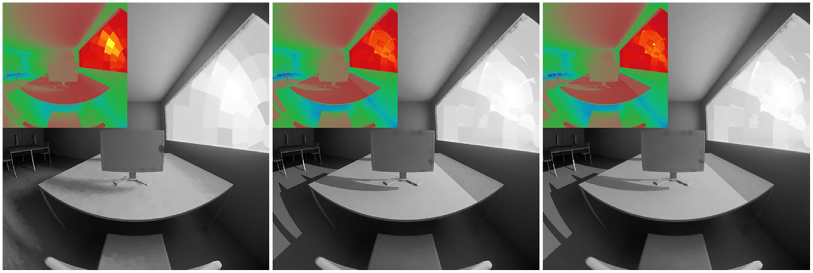
Simulation of an example room with a window equipped with fabric glare protection MS6006 modelled as Klems BSDF. Rendering and luminance false-colour image resulting from simulation without applying the PE method (left), with applying the PE method (centre) and with applying the PE method and a blur filter to mimic a camera lens (right). Note the differences in the sharpness of the interior shadow patterns and the size of the bright area around the solar disc

In order to mimic the measurement using a luminance camera in the simulation, a blur filter based on a Lorentzian function with a full width at half maximum of 11.9 arc min (0.18°) was applied to the rendered images by Ward et al. ¹⁸ (‘A function based on the optical performance of the human eye was used assuming that the scatter is approximately the same as that for the HDR camera lens’). However, this small scatter (0.18°) is not in the order of magnitude that can be achieved with a reasonable BSDF resolution. The right image in Figure 1 shows the result of applying the blur filter to the rendering with PE triggered.

In several validation studies, it has been shown that daylight simulations based on BSDF data can deliver results that match real-world measurements.^25–31 Just recently, Wang et al. have shown that for fabric shades both data-driven BSDF and PE models, as well as isotropic analytical models for simulating fabric shades can lead to results that are consistent between simulations and measurements.^13,32

This however only means that the simulated image and the camera capture match to the extent that the algorithm for extracting the glare sources with then the DGP formula applied lead to comparable results. This in itself is an outstanding achievement. However, it leaves open the question of whether such a high sensitivity for small, very bright light sources in the DGP formula is justified.

Jain et al. ³³ analysed the perceived glare from the sun behind tinted glazing. To avoid a bias in comparisons between different coloured glazings due to effects of the V(λ)-derived luminance-based glare source detection method in evalglare, they implemented a zonal calculation method. Referring to the World Meteorological Organization and the standards organization ASTM International (formerly American Society for Testing and Materials), they average the solar contribution over an area with 2 × 2.9° opening angle (i.e. a solid angle of 0.008 sr). They correctly recognize that this increases the solid angle by a factor of about 100 and reduces the luminance by the same factor, and – due to L ² ω in the formula – that resulting DGP values are thus not comparable to results from other studies. In their study with only relative comparisons, they can accept this.

To cite the last sentence from Section 4.6.2 in Jain et al.’s ³³ paper: ‘Furthermore, there are no studies to the best of our knowledge that investigated the thresholds relevant to (or the algorithms applicable to) determining glare source sizes’.

2. Effect of glare source size: Simulation study

2.1 Method

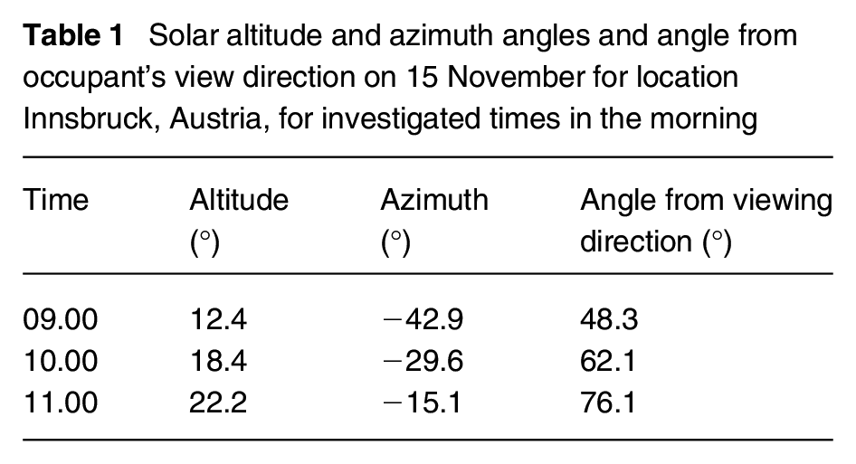
In the first step, we carried out a simulation study to investigate the influence of the size of the glare source. We set up an example test room in Innsbruck, Austria (47.3 N, 11.4 E) with a south-facing window (see Figure 1). We analysed the predicted glare situation for an occupant sitting in this room at the workplace facing east, for a clear sky with sun on 15 November at 09.00, 10.00 and 11.00, respectively. The sun positions at these times are given in Table 1.

Table 1

Solar altitude and azimuth angles and angle from occupant’s view direction on 15 November for location Innsbruck, Austria, for investigated times in the morning

Time	Altitude (°)	Azimuth (°)	Angle from viewing direction (°)
09.00	12.4	−42.9	48.3
10.00	18.4	−29.6	62.1
11.00	22.2	−15.1	76.1

In daylight simulation, especially for annual calculations, fenestration systems are modelled using BSDFs. ⁷ We selected a variety of different BSDFs to represent typical window and shading systems:

1. An electrochromic (EC) window with six different tint states corresponding to visual transmittance at normal incidence of 61%, 42%, 27%, 17%, 7% and 2%, respectively; the system was modelled using the glass modifier in Radiance, and BSDFs were generated using the Radiance genbsdf ³⁴ tool.

2. Eleven light-scattering fabric shades with different weaves, colours and OFs; the BSDF data were generated by Wang et al. ¹³ based on measurements using a scanning goniophotometer pgII ³⁵ and using Radiance BSDF workflow tools³¹; details on the fabrics’ properties are described by Wang et al. ¹³

For all systems, tabulated BSDFs in low-resolution (Klems discretization with 145 × 145 patches, corresponding to an average angular resolution of 2 × 6.7°) as well as in high-resolution (Tensor Tree variable resolution with maximum resolution of 4096 × 4096, corresponding to a minimum angular resolution of 2 × 1.27°) were used. Due to the isotropic behaviour without scattering of glass, isotropic Tensor Tree BSDFs were used for the EC glazing system. The fabric shades, on the other hand, have a strong angular dependence and forward scattering due to their weave and material, which is why anisotropic BSDFs were used. For the EC glazing, we additionally simulated the system as glass material as a reference. All systems were modelled as colour-neutral, that is, existing glare effects due to colour shifts³³ were not taken into account for this study.

The images were rendered with Radiance, version 5.4, using the rtpict tool with ambient caching. To pre-fill the cache an overture simulation with a resolution of 200 × 200 pixel was performed, the final images were rendered at 1200 × 1200 pixel. The simulation parameters were chosen to allow a fast rendering of the images in about 1 min to 2.5 min on a power laptop with an Intel Core i7-12700H with 14 cores (6 Performance-cores, 8 Efficient-cores) and a total of 20 threads. As one ambient bounce is omitted within the direct calculation when using PE, the parameters were adjusted accordingly to make the results comparable:

• rtpict rendering parameters without PE (BSDF material): -ad 1024 -aa 0.03 -ar 50 -ab 3 -ss 0 -lr -6 -lw 1e-7 -dt 0 -st 0

• rtpict rendering parameters with PE (aBSDF material): -ad 1024 -aa 0.03 -ar 50 -ab 2 -ss 0 -lr -5 -lw 1e-6 -dt 0 -st 0

The vertical illuminance E_v was calculated using the rtrace tool in Radiance with high parameter settings to ensure correct consideration of the saturation term in the DGP formula. The rtrace calculation did not use the ambient cache generated by rtpict.

• rtrace simulation parameters without PE (BSDF material): -I -u+ -aa 0 -ab 6 -ad 210000 -dt 0 -ss 0 -st 0 -lw 0 -lr 11

• rtrace simulation parameters with PE (aBSDF material): -I -u+ -aa 0 -ab 5 -ad 210000 -dt 0 -ss 0 -st 0 -lw 0 -lr 10

Figure 2 compares the vertical illuminance values calculated with rtrace to the values reported from the images evaluated with evalglare. Expectedly, while there is no bias in the deviation between the rtrace results based on high parameter settings and the renderings using lower parameter settings, the absolute relative difference is up to 21.6%. The RMSE is 331 lx, which corresponds to a DGP value of 0.019 only due to the saturation term ( $5.87*{10}^{-5}*E_v$ ) in the equation.

Figure 2

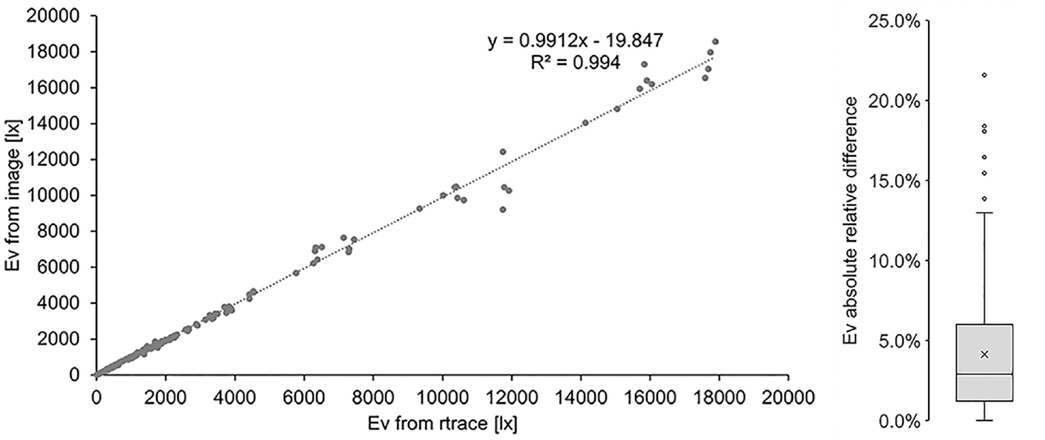
Comparison of vertical illuminance values E_v calculated with rtrace with values reported from renderings evaluated with evalglare. Scatterplot of values (left) and boxplot showing mean and percentiles of absolute relative differences (right)

For this reason, the glare evaluations were done using evalglare in its current version v 2.11 ¹⁹ with the -i option using the vertical illuminance $E_v$ as reported from the rtrace simulation.

For the simulations using the aBSDF material, that is, applying PE, the rendered images were additionally post-processed applying the blur filter as described by Ward et al. ¹⁸ to analyse the effect of this slight blurring and the associated enlargement of the glare source.

2.2 Results

We evaluated the results for all 17 system variants (11 fabric shade systems, 6 glazing states) and for all three points in time. With the different BSDF modelling definitions (with PE, without PE) and discretizations (Klems, Tensor Tree) and additionally the reference glass for EC, in total 222 situations were simulated.

Figure 3 shows the results for the test room with EC glazing in darkest tint state (τ_v = 2.0%) on 15 November at 09.00. For the different variants, the vertical illuminance calculated with rtrace is in good agreement with 337 lx for the reference glass material and between 323 lx and 366 lx for the BSDF versions, for the Klems BSDF and 336 lx for the Tensor Tree BSDF, both without PE. Using aBSDF, PE is triggered for both Klems and Tensor Tree discretizations, resulting in $E_v$ of 366 lx and 336 lx, respectively. However, the expected effect depending on the glare source size is very clear with DGP: from 0.279 for Klems without PE, 0.377 for Tensor Tree without PE and 0.444 for Tensor Tree with PE and blur filter to 0.525 for Klems with PE without blur filter results in all DGP classes (imperceptible below 0.35, perceptible 0.35 to 0.40, disturbing 0.40 to 0.45 and intolerable above 0.45) were obtained.

Figure 3

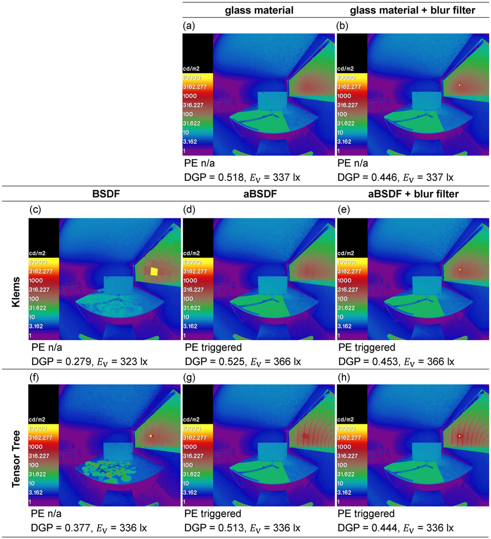
Simulations for sun position on 15 November, 09.00. Top row: Renderings without BSDF using a glass material without blur filter applied (a), and with blur filter applied (b). Middle row: Renderings using a Klems BSDF for EC glazing (τ_v = 2.0%) without PE (c), with PE (d) and with PE and blur filter applied (e). Bottom row: Renderings using an isotropic Tensor Tree g6 BSDF for EC glazing (τ_v = 2%) without PE (f), with PE (g) and with PE and blur filter applied (h)

Results for two different fabric shades are presented in Figures 4 and 5. Fabric MS6006 (τ_v,n-h = 11.0%, OF 3%) in Figure 4 also shows the behaviour of triggering PE for the aBSDF modelling for both Klems and Tensor Tree discretizations for the selected situation on 15 November, 11.00. Due to the underlying, measurement-based BSDF data, there are also deviations in the calculated $E_v$ values. Irrespective of this, the main difference in DGP results is due to the depicted size of the sun, with values ranging from 0.286 (at $E_v$  = 1669 lx) to 0.498 (at $E_v$  = 1569 lx). Results in Figure 5 for fabric MS1901 (τ_v,n-h = 22.7%, OF 5%) show a similar behaviour for the high-resolution Tensor Tree BSDF (bottom row). For the low-resolution Klems BSDF (top row), the PE algorithm is not triggered in this case resulting in equal results for BSDF and aBSDF modelling.

Figure 4

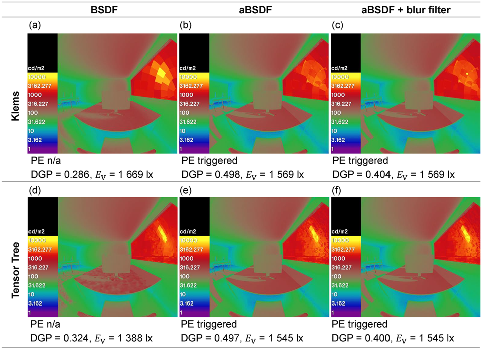
Simulations for sun position on 15 November, 11.00. Top row: Renderings using a Klems BSDF for fabric shade MS6006 (τ_v,n-h = 11.0%, OF 3%) without PE (a), with PE (b) and with PE and blur filter applied (c). Bottom row: Renderings using an anisotropic Tensor Tree g6 BSDF for fabric shade MS6006 without PE (d), with PE (e) and with PE and blur filter applied (f)

Figure 5

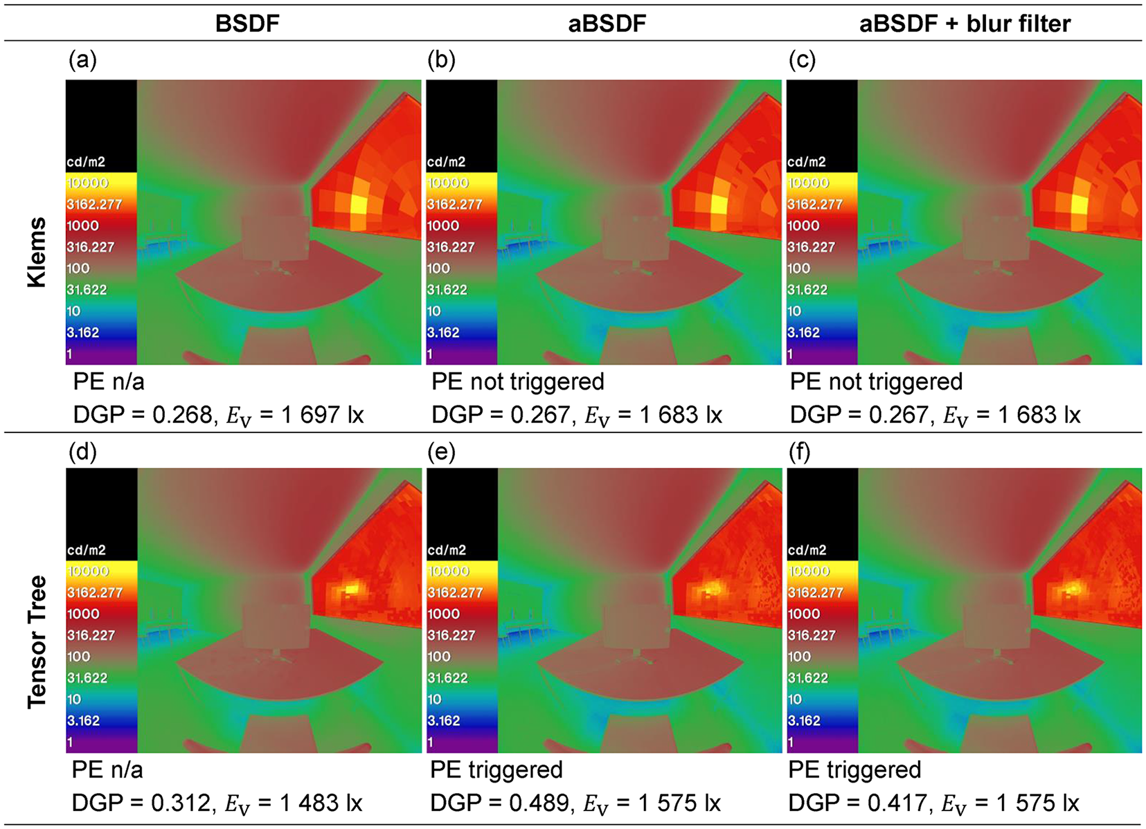
Simulations for sun position on 15 November, 09.00. Top row: Renderings using a Klems BSDF for fabric shade MS1901 (τ_v,n-h = 22.7%, OF 5%) without PE (a), with PE (b) and with PE and blur filter applied (c). Bottom row: Renderings using an anisotropic Tensor Tree g6 BSDF for fabric shade MS1901 without PE (d), with PE (e) and with PE and blur filter applied (f)

3. Perception studies on glare in the peripheral visual field

Expectedly, the results from the simulation study (Section 2.2) show that the DGP formula is highly sensitive to varying glare source sizes. The same occurs with the UGR for evaluating glare from artificial light, where, however, this is taken into account by defining a threshold of 0.0003 sr for the smallest permitted solid angle of a glare source (cf. Section 1.3). Regardless of whether it is artificial light or daylight, the following question arises: If two glare sources, causing the same vertical illuminance at an observer’s eye but differing in size (and therefore differing in brightness) cannot be distinguished, should not a glare evaluation metric applied to these sources yield consistent evaluations?

For the DGP, there is currently no established method for taking into account small glare sources such as direct sunlight penetrating through glare protection devices or small, bright areas in daylight systems due to specular reflections or refraction. There is also no method comparable to CIE 232 for evaluating inhomogeneous luminance structures, which occur in the daylight area, for example due to structures in daylight systems.

3.1 Method

The initial aim was to determine the size at which small light sources in the periphery, which cause equal vertical illuminances, are no longer distinguishable and thus provide evidence that the glare effect should also be comparable. The first step was thus to determine the minimum solid angle (i.e. the cone with an opening angle $2\times {\gamma }_{\mathrm{threshold}}$ ) that justifies an evaluation with $L^2\omega$ when applying the DGP formula (Equation (1)) for daylighting situations, or vice versa, the size below which the rating may no longer change. Therefore, we investigated the size at which a visual stimulus in the peripheral visual field can be clearly distinguished from smaller visual stimuli.

For this purpose, participants were shown circular discs on an ultra-high brightness screen (DynaScan DS55LT6, Full HD resolution 1920 × 1080) in 2 m distance, which can display a luminance of up to 5000 cd m⁻². Five horizontal viewing directions (30°, 45°, 60°, 75° and 90° to the right) and three vertical viewing directions (30°, 45° and 55° downwards) were tested. For objectifiable results, random pairs of circular discs were presented, which generated the same vertical illuminance at the eye. The order of the viewing directions was randomized to minimize learning effects. Statistical analysis was used to determine the size ratios at which a test subject reliably recognizes the differences.

A disc diameter of 550 pixels at a distance of 2 m from the participant corresponds to a solid angle of a cone with aperture 2 × 5°. The diameter of the discs is chosen to have approximately factors of 2 in the area between adjacent discs sizes. Thus, there is also a factor of 2 concerning solid angle $\omega =2\pi (1-\cos \gamma )$ and the vertical illuminance at the eye $E_v=L\pi \mathrm{si}{\mathrm{n}}^2\gamma$ at equal luminance. Table 2 shows selected disc sizes and corresponding opening angles.

Table 2

Selected disc sizes and corresponding opening angles for presentation on ultra-high brightness display

Disc diameter (pixel)	24	34	50	70	98	138	194	274	390	550	778	1080
Cone 2 × γ (°)	0.22	0.31	0.46	0.64	0.89	1.26	1.77	2.49	3.55	5.00	7.05	9.74

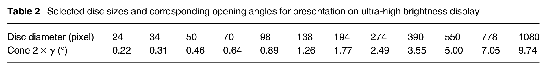
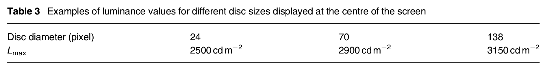
The luminance of the disc that can be achieved on the display depends on the size of the disc and its position on the screen. The full luminance of the screen can only be achieved by having the full screen set to maximum (R, G, B = 255). Maximal possible luminances for different disc sizes were measured with a Minolta luminance meter. Examples for discs in the centre of the screen are given in Table 3.

Table 3

Examples of luminance values for different disc sizes displayed at the centre of the screen

Disc diameter (pixel)	24	70	138
L max	2500 cd m−2	2900 cd m−2	3150 cd m−2

Using different calibration curves for the five possible positions of the discs on the screen (centre, left, right, up, down), it was possible to guarantee that the luminance is at maximum for the smallest disc in the experiment and that the discs shown in one experiment produce equal vertical illuminances at the observer’s eye.

For each person and each viewing direction, four circular disc diameters were determined individually in a preliminary run. This allowed to reduce the total number of tests per person and limit them to the relevant disc sizes. In the actual tests, the smallest of these four circular discs was compared with one of the four discs to determine when the differences in size could be recognized. The viewing directions and the sizes of the circular discs were randomly permuted to avoid learning effects. Two different experimental designs were prepared: In the first, the size of the discs was changed continuously, and in the second, two discs were presented simultaneously. Figure 6 shows a fisheye photograph of the experimental setup, and Figure 7 shows the display in experimental design 2 and the red marks for the horizontal viewing directions. Figure 8 shows a perspective view together with a floor plan and a cross-section of the experimental layout.

Figure 6

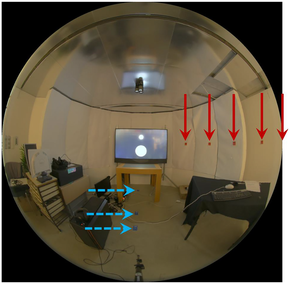
Predefined horizontal (red; 30°, 45°, 60°, 75° and 90°) and vertical (blue, dashed; 30°, 45° and 55°) viewing directions

Figure 7

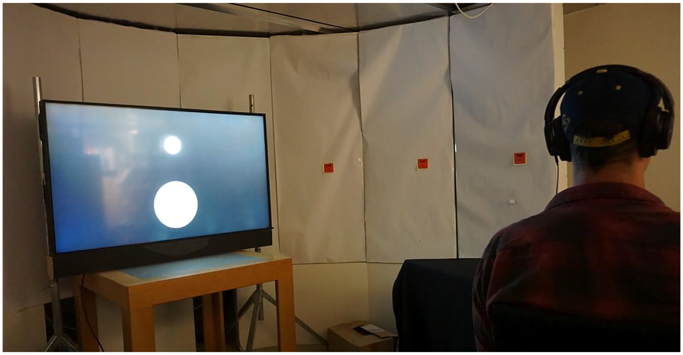
Display presenting circular discs in the peripheral visual field in experimental design 2 with simultaneous presentation of discs. Red marks indicate the horizontal viewing directions (visible in image: 30°, 45° and 60°)

Figure 8

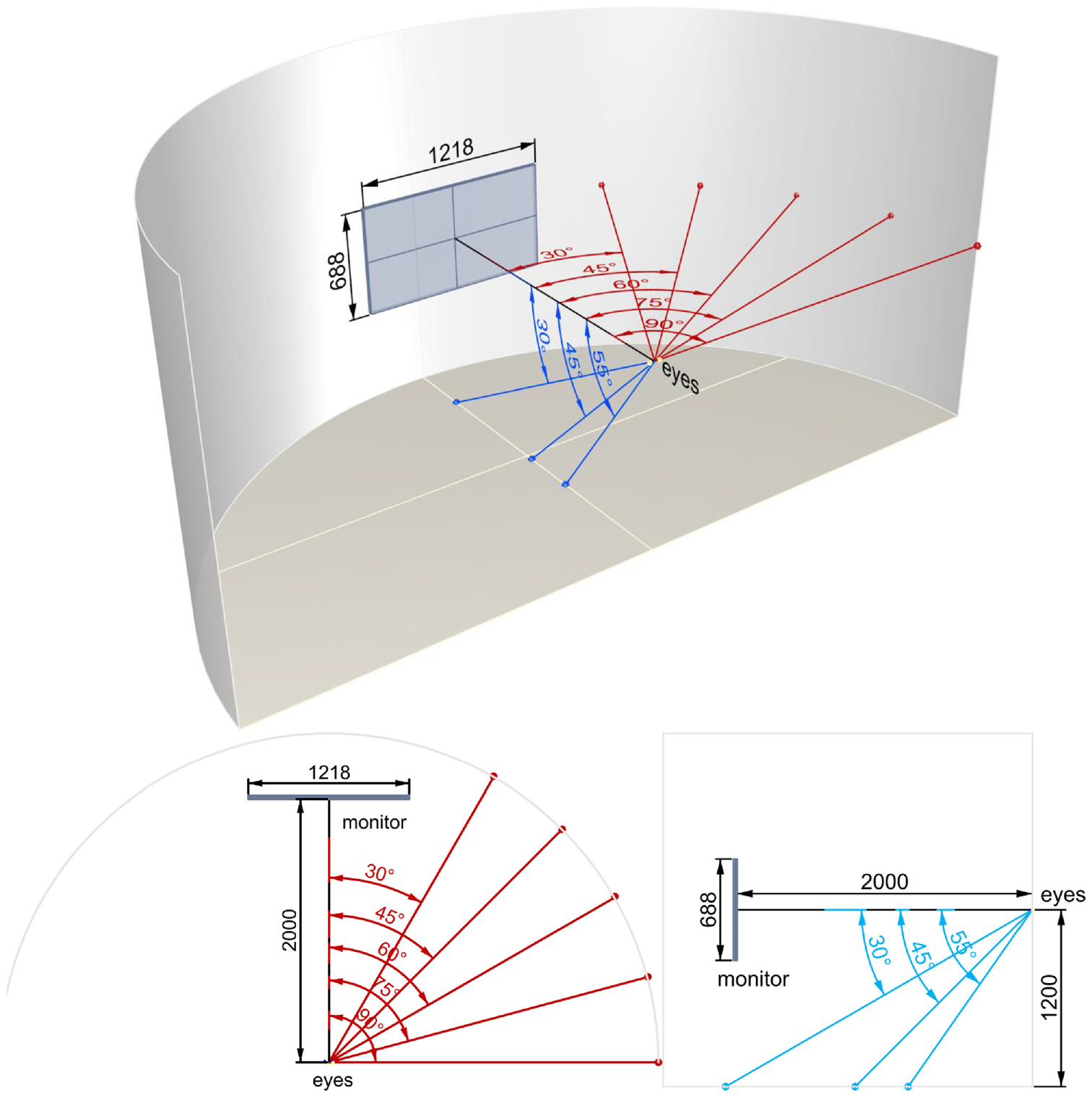
Experimental layout: perspective view (top), floor plan (bottom left) and cross-section (bottom right)

3.1.1 Experimental design 1: Continuous change in size of the circular discs

The visual task is to distinguish between a small, bright circular disc and a large, darker one, both of which generate the same vertical illuminance. This is achieved by continuously changing the diameter d and the luminance L of a circular disc in the centre of the screen while keeping the vertical illuminance at the eye $E_v~L{d}^2$ constant (Figure 9).

Figure 9

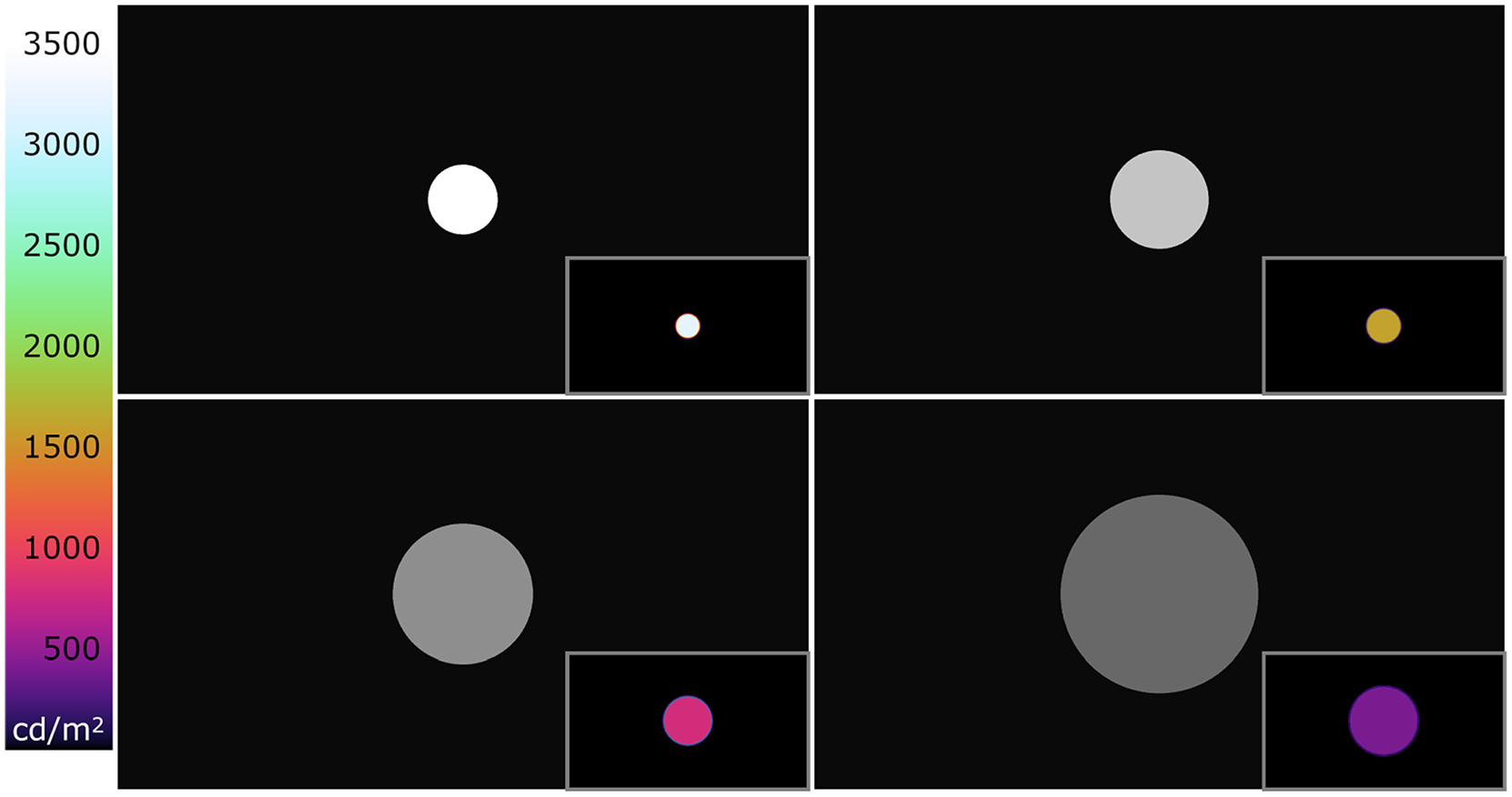
Examples of circular discs on the monitor in experimental design 1 with continuous size change. Small inlays show false-colour presentations of the luminance values 3200 cd m⁻², 1604 cd m⁻², 792 cd m⁻² and 398 cd m⁻², respectively

The first idea was to show the two visual stimuli one after the other. The assumption that the sudden change facilitates recognition led to the following adjustment. By using a continuous transition between the two circular discs, it was possible to avoid a dark phase between the presentation of the first and the second circular disc. During the whole transition, the vertical illuminance was kept constant. The participants had to decide whether the visual stimulus becomes larger or smaller or remains the same size.

This preliminary study involved 14 people (11 male, 3 female) between the ages of 22 and 58. Most participants carried out the tests several times, resulting in 32 performed experiments. One experiment consisted of (5 + 3) × 6 × 2 × 4 × 2 = 768 comparisons of discs:

• 5 + 3 randomized viewing directions, repeated six times

• 2 × 4 comparisons (sizes 1:1, 1:2, 1:3, 1:4) and reverse, randomized

• Repeated twice per viewing direction.

In total, there have been 24 576 comparisons of discs.

3.1.2 Experimental design 2: Simultaneous presentation of circular discs with different size

The visual task again was to distinguish between a small, bright circular disc and a large, darker one, both of which generate equal vertical illuminance at the eye. Both discs are always of different sizes and thus different luminances (Figure 10). The participants were asked to spot the position of the small, bright disc. This study included 11 people (10 male, 1 female) aged between 23 years and 58 years. One experiment consisted of (5 + 3) × 6 × 2 × 3 × 2 = 576 comparisons of discs:

• 5 + 3 randomized viewing directions, repeated six times

• 2 × 3 = 6 comparisons (sizes 1:2, 1:3, 1:4) and reverse, randomized

• Repeated twice per viewing direction

In total, there have been 6336 comparisons of discs.

Figure 10

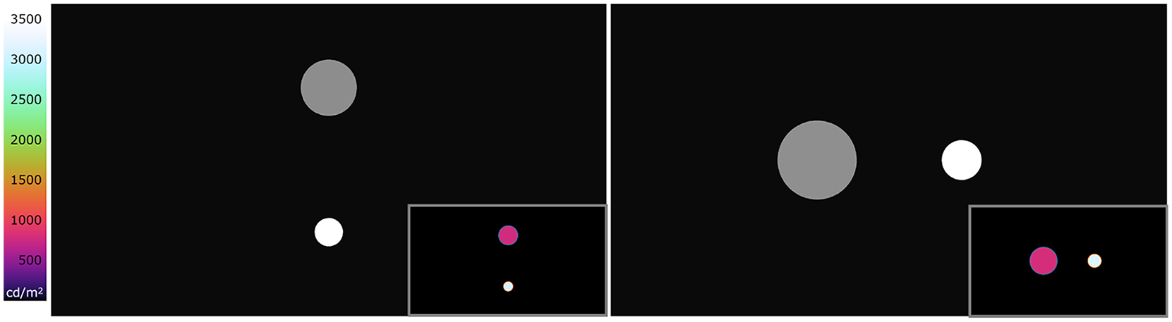
Examples of circular discs in experimental design 2 for viewing direction horizontally to the right (left image) and vertically downwards (right image). Small inlays show false-colour presentations of the luminance values 778 cd m⁻² and 3050 cd m⁻² (left), and 799 cd m⁻² and 3150 cd m⁻² (right)

3.2 Results

In the studies (experimental designs 1 and 2 are described in Sections 3.1.1 and 3.1.2, respectively) we determined the size (i.e. minimum solid angle defined through the cone with an opening angle $2\times {\gamma }_{\mathrm{threshold}}$ ) at which small light sources in the periphery are no longer distinguishable. The results indicate that the threshold angle to distinguish small sources, especially in the periphery of the field of vision is larger than it has been assumed up to now. Particularly in the periphery, even large differences in size could not be distinguished from one another according to subjective assessment. From the perception studies, we determined threshold angles γ_threshold for both horizontal and vertical viewing directions, with the latter being significantly larger. Compared to the visual acuity angles that are used in CIE 232, ²³ both are considerably larger, that is, even significantly larger glare sources could not be distinguished in the tests. Moreover, the angles calculated according to the method proposed in CIE 147 ²² are smaller than the obtained vertical threshold angles. Figure 13 shows the threshold angles derived from both experiments (cf. Figures 10 and 12) together with reference angles.

Figure 11

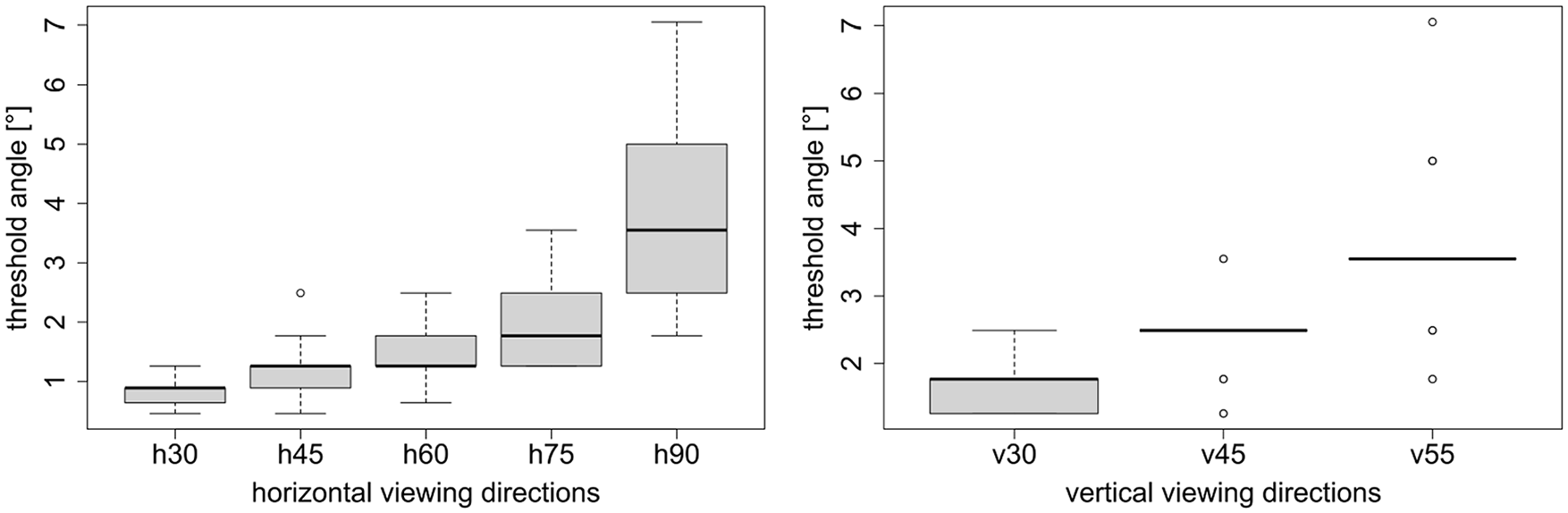
Experimental design 1: resulting threshold angles for horizontal viewing directions 30°, 45°, 60°, 75° and 90° (left), and for vertical viewing directions 30°, 45° and 55° (right)

Figure 12

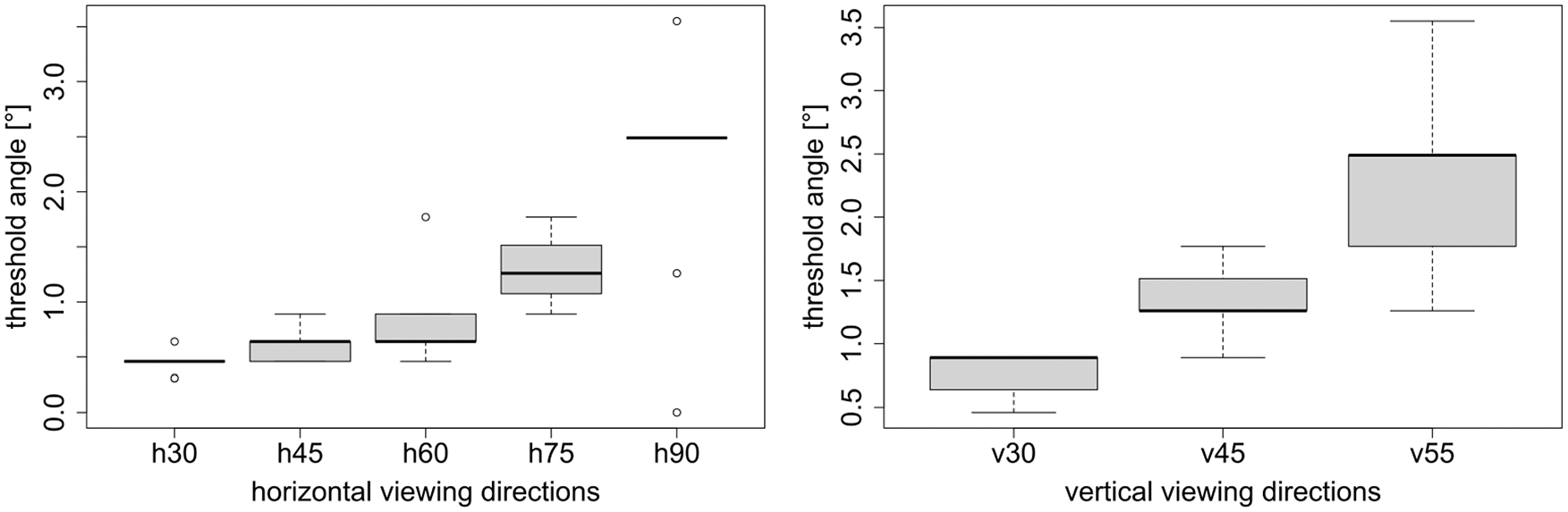
Experimental design 2: resulting threshold angles for horizontal viewing directions 30°, 45°, 60°, 75° and 90° (left), and for vertical viewing directions 30°, 45° and 55° (right)

Figure 13

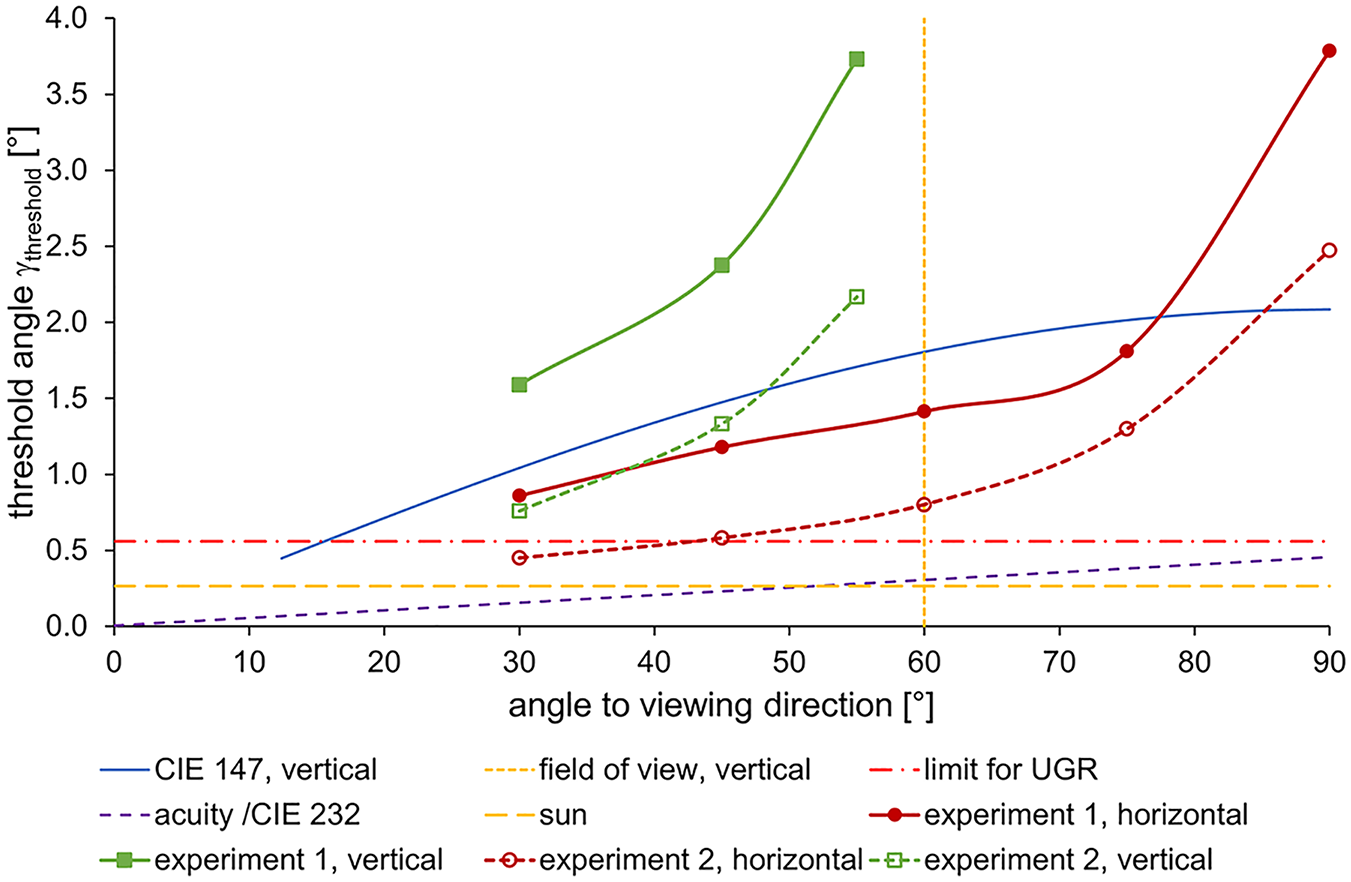
Threshold angles γ_threshold derived from perception studies 1 and 2, angles for visual acuity according to CIE 232, angles obtained from the procedure in CIE 147 and limit as specified for UGR calculation

The results were used to modify the DGP metric to consider the effects concerning the detection of size differences in peripheral vision studied in the two experimental designs.

The concept of the adapted glare rating is to replace the solid angle for glare sources with opening angle smaller than $2\times {\gamma }_{\mathrm{threshold}}$ by ${\omega }_{*}=2\pi (1-\cos {\gamma }_{\mathrm{threshold}})$ . At the same time, the luminance is replaced by the luminance $L_{*}$ averaged over this solid angle ${\omega }_{*}$ to preserve the illuminance at the observer’s eye, that is, also an equal illuminance $E_{\perp }$ perpendicular to the direction of the glare source. For a source that is a cone with opening angle 2 × γ,

$$E_{\perp }=L\pi \mathrm{si}{\mathrm{n}}^2\gamma =L_{*}\pi \mathrm{si}{\mathrm{n}}^2{\gamma }_{\mathrm{threshold}}$$

(2)

and thus

$$L_{*}=L\frac{\mathrm{si}{\mathrm{n}}^2\gamma }{\mathrm{si}{\mathrm{n}}^2{\gamma }_{\mathrm{threshold}}}$$

(3)

For small solid angles this can be replaced by

$$L_{*}=L\frac{\omega }{{\omega }_{*}}$$

(4)

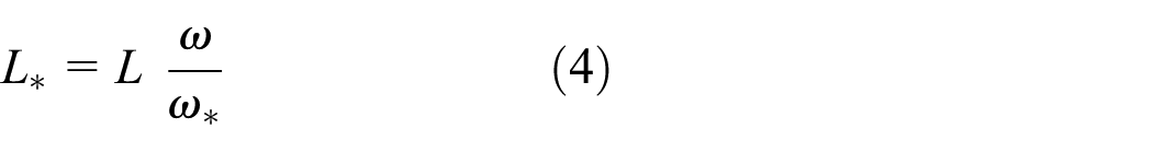
Finally, L ² ω in DGP is replaced by

$$L_{*}^2{\omega }_{*}=L^2\frac{{\omega }^2}{{\omega }_{*}^2}{\omega }_{*}=L^2\frac{{\omega }^2}{{\omega }_{*}}$$

(5)

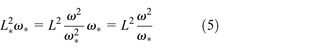
to obtain the modified DGM (Equation (6)):

$$\begin{array}{cc}\multicolumn{1}{c}{\mathrm{DG}{\mathrm{P}}_{\mathrm{modified}}}& =\mathrm{DGM}=5.87\times {10}^{-5}{E}_v+0.0918\hfill \\ \multicolumn{1}{c}{}& \times \log (1+\sum \frac{L_{s,i}^2{\omega }_i^2}{E_v^{1.87}{p}_i^2{\omega }_i^{*}})+0.16\hfill \end{array}$$

(6)

Comparing the results of our experiments with the CIE 147 values and the UGR limit, we decided to base this first proposed modification on the results of experiment 2, which is not only closer to the references mentioned but also causes a less aggressive change in the metric. The threshold angles were thus defined based on experiment 2 introducing an additional factor $\mathrm{scal}{\mathrm{e}}_{\mathrm{threshold}}$ . For $\mathrm{scal}{\mathrm{e}}_{\mathrm{threshold}}=1$ , the results from experiment 2 were fitted with TuringBot 2.16.1, ³⁶ a software using symbolic regression to find mathematical formulas from data values. The following formula for the threshold angle has been chosen (Equation (7)):

$$\begin{array}{c}{\gamma }_{\mathrm{threshold}}=\mathrm{scal}{\mathrm{e}}_{\mathrm{threshold}}\hfill \\ \times [{(\cos \alpha (\beta -0.230914)+\beta -0.284456)}^{2.02609\beta }+0.238658]\hfill \end{array}$$

(7)

with α, β (rad), γ_threshold (°), where α and β are the angles defined according to Figure 14.

Figure 14

Angles α and β used in formula for threshold angle ${\gamma }_{\mathrm{threshold}}$

For $\cos \alpha (\beta -0.230914)+\beta -0.284456\le 0$ we set ${\gamma }_{\mathrm{threshold}}=\mathrm{scal}{\mathrm{e}}_{\mathrm{threshold}}\times 0.238658$ . We propose to use a scaling factor $\mathrm{scal}{\mathrm{e}}_{\mathrm{threshold}}=2.346$ . This limits the solid angle up to ~15° from the viewing direction so that the solid angle is 0.0003 sr, that is, matches the limit specified for the UGR calculation. Additionally, an upper limit ${\gamma }_{\mathrm{threshold}}\le 6.{552}^{°}$ is defined that holds primarily outside the field of view (see Figure 15). For the lower hemisphere, the same formula for the threshold angle is applied and even there the solid angle is at least 0.0003 sr. As no experimental data are available, the DGM should however be used with care for glare sources below the horizon or the line of sight.

Figure 15

Proposed threshold angle ${\gamma }_{\mathrm{threshold}}$ derived from results of experimental design 2, including the proposed scaling factor $\mathrm{scal}{\mathrm{e}}_{\mathrm{threshold}}=2.346$

3.3 Evaluation of the modified metric DGM

We evaluated all 222 simulations of the simulation study (Section 2) using the DGM (i.e. modified DGP) formula from Equation (6) with the proposed scaling factor $\mathrm{scal}{\mathrm{e}}_{\mathrm{threshold}}=2.346$ in Equation (7), and compared it with DGP. Additionally, all images were post-processed using the blur filter ¹⁸ and evaluated with the DGM and DGP methods again. The results based on the images with blur filter are referred to as DGP* and DGM* in Figures 16 to 21.

Figure 16

Glare metrics evaluated for simulations of test room with EC glass under CIE clear sky with sun in Innsbruck, Austria, 15 November, 09.00

Figure 17

Glare metrics evaluated for simulations of test room with EC glass under CIE clear sky with sun in Innsbruck, Austria, 15 November, 10.00

Figure 18

Glare metrics evaluated for simulations of test room with EC glass under CIE clear sky with sun in Innsbruck, Austria, 15 November, 11.00

Figure 19

Glare metrics evaluated for simulations of test room with fabric shades under CIE clear sky with sun in Innsbruck, Austria, 15 November, 09.00

Figure 20

Glare metrics evaluated for simulations of test room with fabric shades under CIE clear sky with sun in Innsbruck, Austria, 15 November, 10.00

Figure 21

Glare metrics evaluated for simulations of test room with fabric shades under CIE clear sky with sun in Innsbruck, Austria, 15 November, 11.00

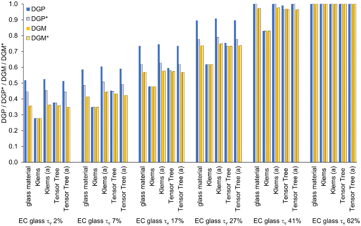
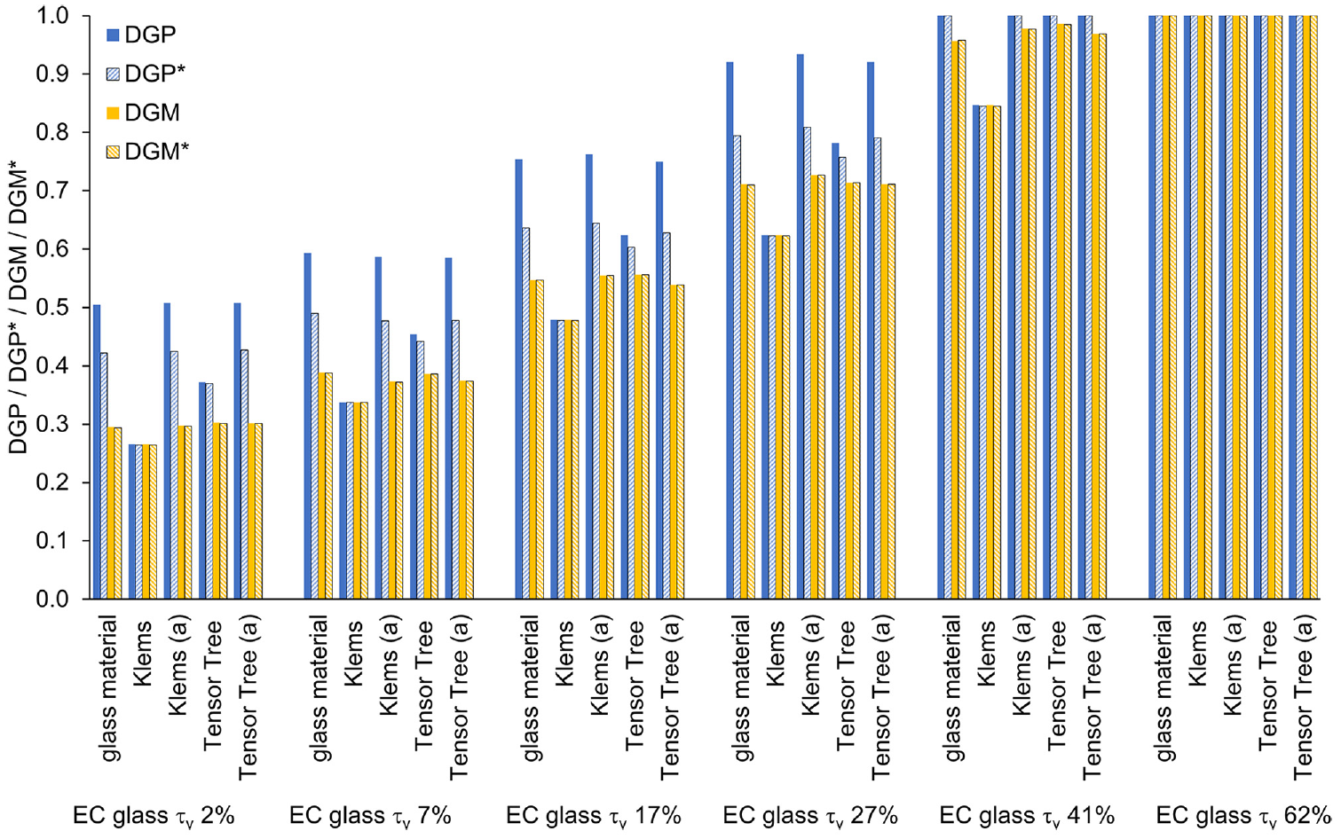
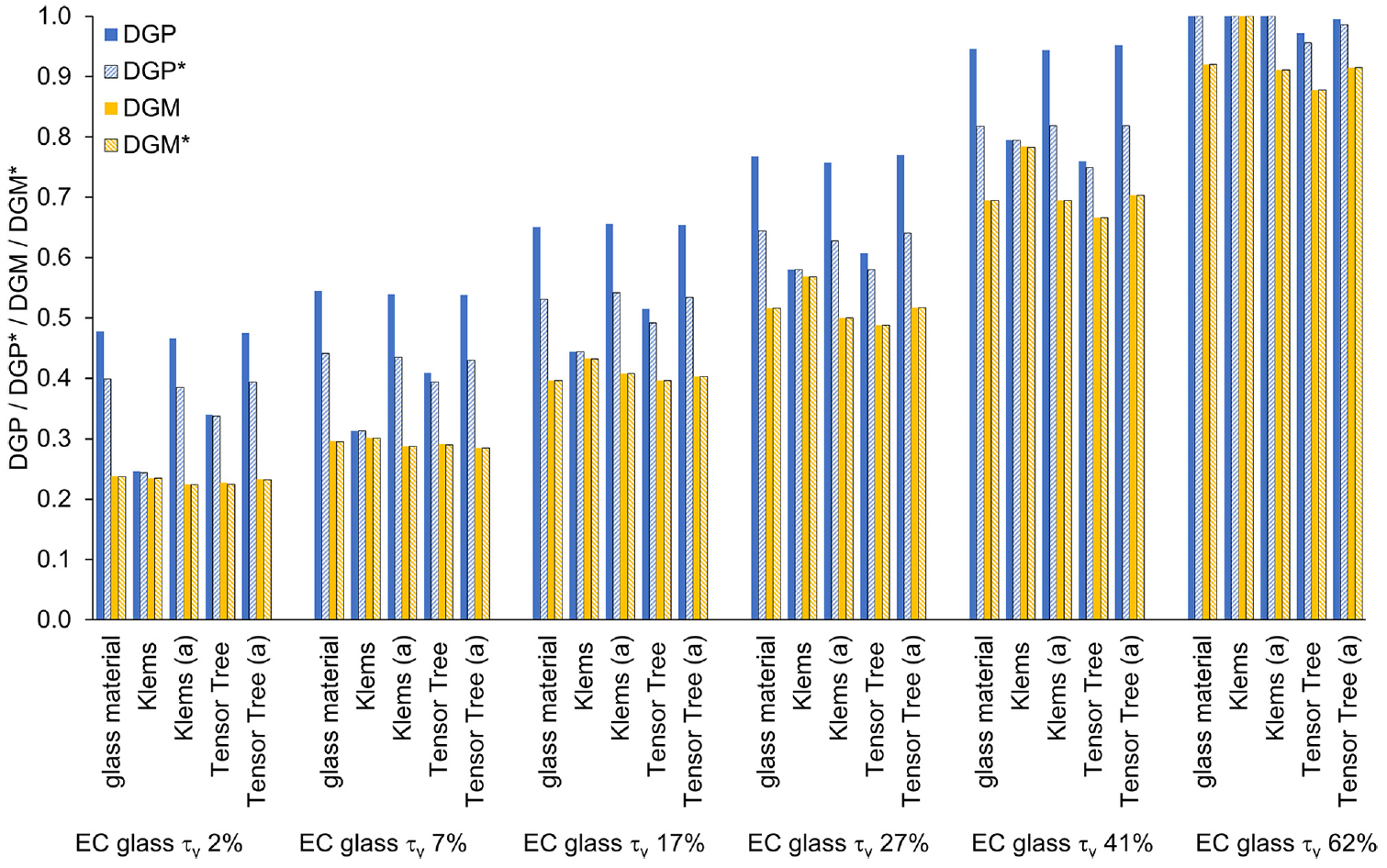
3.3.1 EC glazing

We first look at the results for the scenes with EC glazing in the six different tint states 2%, 7%, 17%, 27%, 41% and 62% (Figures 16 to 18). For each state, the left group of bars shows the results for the reference case (i.e. glazing modelled as Radiance glass material). Furthermore, the results for the glazing modelled as BSDF in Klems resolution are shown in the second (BSDF material) and third groups (aBSDF material; labelled (a)). The fourth and fifth groups show the corresponding results for high-resolution Tensor Tree BSDFs.

The influence of the rendered size of the sun can be clearly seen in the results. For the 2% state at 09.00, for example, DGP in the reference case (glass material) is 0.518, while it is only 0.279 when using the Klems BSDF, or 0.377 when simulating with the Tensor Tree BSDF, respectively. For all situations, PE is always triggered for the EC glass when modelling it as aBSDF material, that is, the sun is always rendered at its real size with 2 × 0.26° opening angle. This is also independent of whether Klems or Tensor Tree discretization is used. The resulting DGP values for the 2% case are 0.525 (Klems as aBSDF) and 0.513 (Tensor Tree as aBSDF), respectively, and thus in very good agreement with the reference.

The significant influence on the DGP results of the application of the blur filter in scenes with tiny sources, that is, the sun in its real size, can be clearly seen. For the above example (2% tint, 09.00), DGP decreases from 0.518 to 0.446 in the reference case (glass material), from 0.525 to 0.453 (Klems aBSDF) or from 0.513 to 0.444 (Tensor Tree aBSDF). The other results are barley affected (from 0.279 to 0.278 for Klems, from 0.377 to 0.375 for Tensor Tree).

However, if we look at the DGM results, we see that the metric stabilizes for sufficiently small representation of the sun. While Klems distributes the luminous flux over a too large solid angle resulting in a DGM of 0.279, the results for the reference, Klems (a), Tensor Tree and Tensor Tree (a) match very well with 0.358, 0.364, 0.359 and 0.350, respectively. As small light sources are already assumed larger in the algorithm for the DGM, the blur filter has no significant influence on the DGM results (additional reduction of about 0.001 to 0.006).

The effects described are comparable for all variants and situations with EC glass. One exception to this is the effect that the results for Klems without PE are slightly higher than with PE for the situation at 11.00. This is due to the position of the sun and its position in the associated Klems patch. This causes the glare source to be blended much further towards the centre.

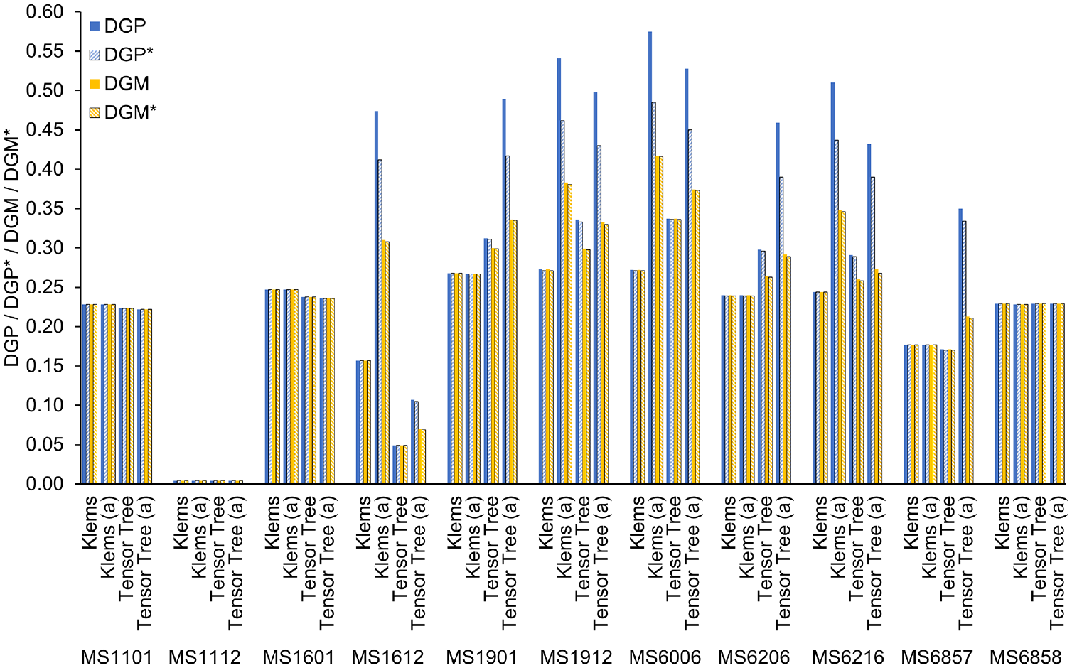
3.3.2 Fabric shades

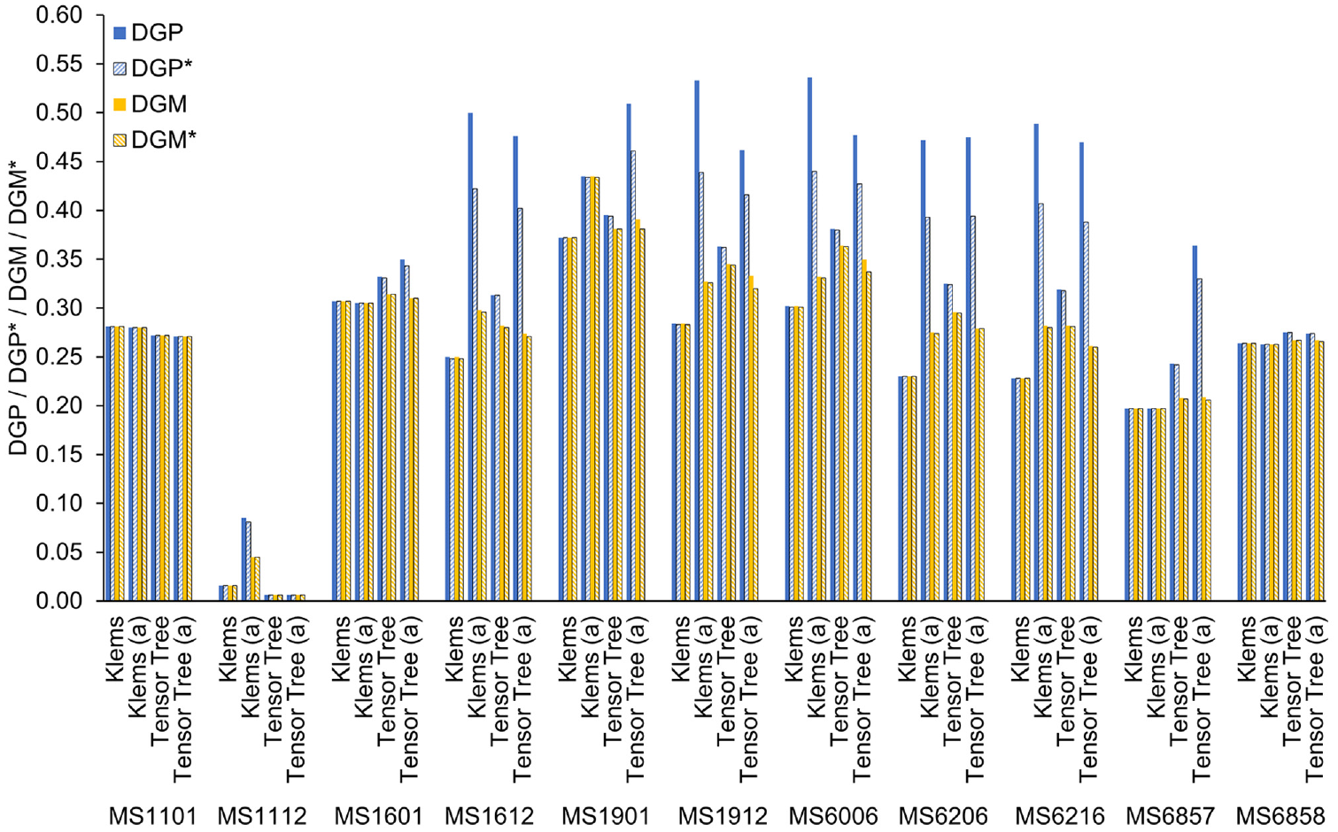
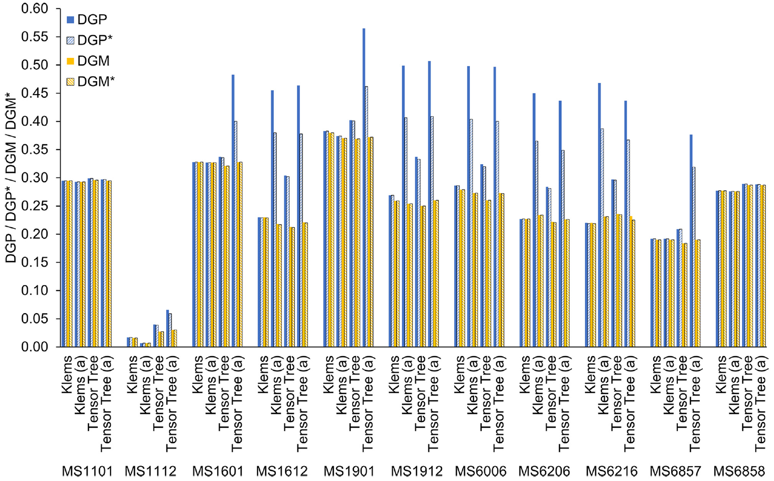
The results for the fabric shades (Figures 19 to 21) show that the behaviour of the systems differs depending on their transmission, OF and structure-dependent cut-off angle.

For systems MS1101 and MS6858, PE is never triggered, that is, no direct solar input is recognized in the algorithm; thus, the results of the modified DGM match the original DGP. For fabric MS1112, a dark fabric with small OF, all reported glare values are below 0.1, that is, below the range where meaningful glare evaluation is possible.

For all other systems, it can be seen that whenever PE is triggered, the resulting DGP values predict significant glare with values that are also significantly higher than predicted when using the high-resolution Tensor Tree BSDF without PE. This predicts clear differences for glare light sources with aperture angles of 2 × 0.26° or 2 × 1.27°, which are clearly in the periphery.

With the DGM, this difference is also present, but not as pronounced and only for the situations at 09.00 and 10.00. At 11.00, where the sun is very peripheral in the field of view (angle from viewing direction 76.1°), the reported DGM values are in very similar ranges for both discretizations Klems and Tensor Tree, with and without PE, respectively. This clearly underlines the results from the studies that the size of the glare sources has hardly any influence in the periphery.

4. Outlook and discussion

Both test setups (experimental designs 1 and 2) allow the investigation of the limited ability to distinguish between stimuli of different sizes that produce the same vertical illuminance on the eye, especially in the peripheral field of view. However, the visual environment and the light stimuli in these tests do not correspond to real daylighting situations. It is thus essential to verify the modification of the DGP with tests in an appropriate visual environment.

In a follow-up study, additional perceptual-psychological tests will be carried out under an artificial sky with an artificial sun (LED luminaire) as glare source to mimic real daylight situations more closely (illuminance from surroundings $E_v$  = 1000 lx, glare sources luminance of up to 6000 kcd m⁻²).

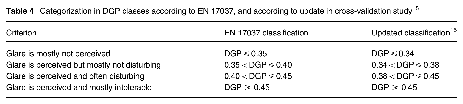
The study design was already developed and a pilot study with internal participants performed (see Figure 22). A total of 16 situations will be presented where the position of the source changes widely in the field of view with azimuth angles of 0°, 20°, 45° and 70° and elevation angles (height) of 20°, 30°, 35° and 40°. The luminance of the source ranges from 375 kcd m⁻² up to 6000 kcd m⁻² (375 kcd m⁻², 750 kcd m⁻², 1500 kcd m⁻², 3000 kcd m⁻², 6000 kcd m⁻²). The situations were selected to show cases where the DGM and DGP ratings differ and fall into different classes according to Table E.1 in EN 17037 (see Table 4), as well as cases where DGP and DGM are equal.

Figure 22

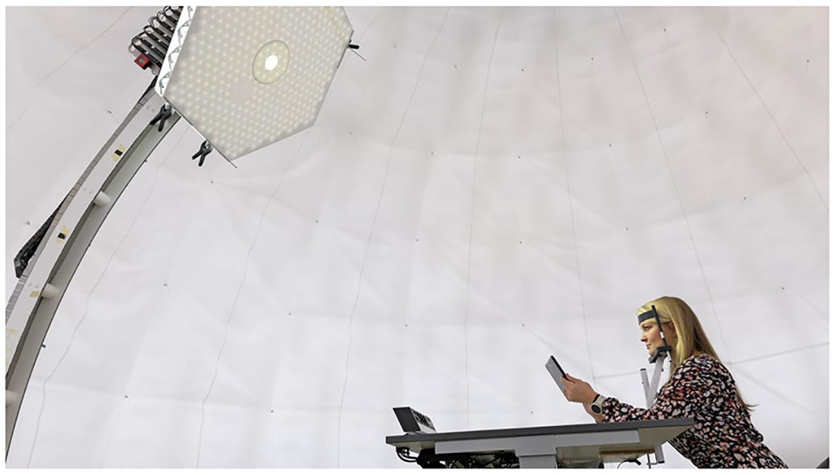
Setup of the pilot study for the upcoming DGM validation study under an artificial sky and sun

Table 4

Categorization in DGP classes according to EN 17037, and according to update in cross-validation study ¹⁵

Criterion	EN 17037 classification	Updated classification 15
Glare is mostly not perceived	DGP ≤ 0.35	DGP ≤ 0.34
Glare is perceived but mostly not disturbing	0.35 < DGP ≤ 0.40	0.34 < DGP ≤ 0.38
Glare is perceived and often disturbing	0.40 < DGP ≤ 0.45	0.38 < DGP ≤ 0.45
Glare is perceived and mostly intolerable	DGP ≥ 0.45	DGP ≥ 0.45

Test case examples contain situations where DGP = DGM = 0.45, or where DGP = 0.53 while DGM = 0.40. Figure 23 shows a selection of the intended situations. The start is a reference situation with intolerable glare (source size 2 × 1.05°, $L_S$  = 6000 kcd m⁻², DGP = 0.69, DGM = 0.62) to have the same situation at the beginning as a calibration for all participants.

Figure 23

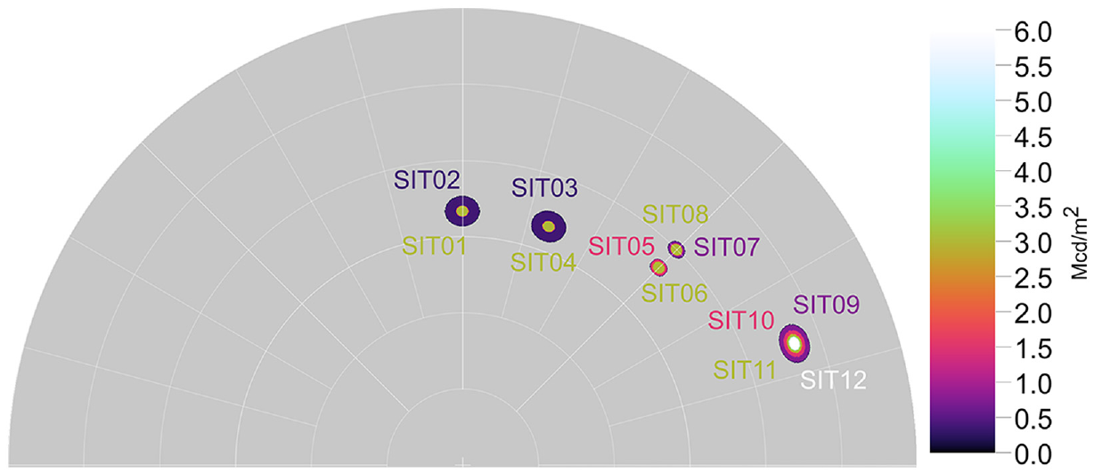
Selection of proposed situations (viewing directions, solid angles and luminances) in the design for the DGM validation study under the artificial sky and sun

This study is aimed to investigate whether the DGM corresponds better with the judgement of the test participants than the original DGP. Additionally, it should allow to check if the adjustment (especially the chosen scaling factor) must be adapted to these results.

As a first indication from the pilot study, effects are as expected. For example, for situations where the azimuth of the sun is 70°, there was no significant difference in the glare assessment of the test persons. This matches with the modified DGP results which are DGM = 0.40 for all these situations, while the original DGP increases from 0.45 to 0.53. These first results indicate that especially in the periphery of the field of view, small glare sources below a threshold angle do not cause more glare than larger glare sources that generate the same vertical illuminance. It is essential to take this effect into account so that the actual glare judgements of test participants correspond optimally with the modified glare metric.

As an alternative to the approach used for the DGM, also a corresponding Gaussian filter on the luminance picture could be applied before calculating DGP. This approach would be similar to the method described for artificial lighting in CIE 232. ²³ The advantage of the DGM is that no post-processing of the luminance picture is necessary. In addition, the DGM corresponds exactly to the classic DGP in cases where the glare source size is not below the threshold. This means that existing evaluations and specifications remain valid for these situations.

In the simulation study, we have seen that there are cases where the triggering of PE depends on the BSDF discretization. In some of these cases, the DGM method achieves that the evaluation does not differ between high-resolution BSDF simulations with and without PE, especially for glare sources in the peripheral field of view. However, it is worth considering whether the PE method can be further refined to achieve even better agreement when PE is triggered.

5. Conclusions

We presented an overview of the status of daylight glare assessment using DGP in current standards and showed why small glare sources pose a problem in the metric. Comparable issues are known from the field of artificial lighting (UGR metric), but are solved there through the definition of threshold values or adaptation and extension of the calculation methods (e.g. CIE 147 or CIE 232). We also gave an overview of tools that have recently been developed to perform daylight simulations and glare assessments. The focus here is clearly on the challenge of being able to properly represent shading and daylighting systems using BSDF data.

The results of the simulation study highlight why the critical analysis of the DGP metric for small, bright glare sources like the sun is of highest relevance. For tinted glazing as well as various fabric shades, we could show that depending on the used BSDF data resolution and the applied methods (with or without PE), the resulting DGP values vary significantly and can jump even between imperceptible to intolerable glare ratings. This prompted us to carry out a study to determine the distinguishability of small glare sources, particularly in the peripheral visual field. We were able to derive an adjustment to the DGP metric from the results of the subject study, which is based on the introduction of a position-dependent threshold for the minimum size of a glare source. We then evaluated the simulation study results using the modified DGM. For situations with small bright glare sources such as the sun in the field of view, the new metric stabilizes the results over different underlying data resolutions or simulation methods. Without small glare sources, the adapted metric matches the classical DGP results. We finally discussed that further tests need to be performed under daylight-like conditions to validate the adjusted metric.

Adoption of the DGM – possibly adapted after the further tests – into the relevant standardization is highly recommended as it is more robust against variations in the underlying data and methods. Irrespective of this, the standards should contain precise instructions on how to carry out the standardized daylight glare assessment. This includes specifying which methods and threshold values are used to extract glare sources from a luminance picture and which parameter settings are to be used in the glare evaluation software. Even if in some cases the optimum settings for the respective situation are certainly not achieved, this is absolutely necessary in terms of standardization to ensure comparability.