Sage Journals: Discover world-class research

Abstract

The effect of a 13-week exposure to moderate levels of light modulation resulting in visible, but not irritable, stroboscopic effect was studied. Over the course of three months, two sets of participants working in an office environment filled in a questionnaire about their health and wellbeing at the start and the end of each working day. Using a schedule of changes between two light settings differing only in the amount of temporal modulation, it was shown that the higher temporal modulation light did not significantly increase the occurrence of any health and wellbeing parameters (like eyestrain and headaches) tested. Furthermore, even though there was a large variation in the individual probability of complaints, there was no interaction effect between the individual level of complaints and the amount of light modulation. Using power analysis, we demonstrate that the increase of unwanted effects of 5% or more has a probability of less than 5%.

1. Introduction

Deliberate temporal modulation (e.g. pulse width modulation) of a light source’s output can be used for predictable control of the intensity and colour of the produced light but can also introduce new problems. Most notably, temporal modulation can lead to unwanted changes in the perception of the environment, called temporal light artefacts (TLA). The two most relevant TLAs for office applications, the applications of interest in this work, are flicker and the stroboscopic effect. Flicker is the direct observation of the temporal modulation, and it is visible to a frequency of about 80 Hz.¹ The stroboscopic effect is a spatio-temporal effect that is a result of the interaction of temporally modulated light with visibly moving objects in the field of view of the observer. Technical definitions and guidelines for measuring the visibility of those effects can be found in International Commission on Illumination (CIE) Publication 006:2016.²

Contrary to the unwanted visual effects of temporally modulated light, the adverse health and wellbeing effects have been less studied. Long-term exposure studies are particularly lacking. The visual effect that is most often indicated in causing adverse biological effects and most often studied is flicker. Light stimuli, temporally modulated at 10 Hz to 20 Hz, can trigger migraine attacks, and migraine is the most prevalent neurological disorder in the general population.³ In patients suffering from photosensitive epilepsy, which is the most common form of stimulus-induced epilepsy, exposure to flickering light can trigger a seizure with the most epileptogenic being modulations at frequencies of 5 Hz to 10 Hz.^4,5 Stimulation with flickering stimuli has been used in clinical studies to examine a variety of abnormal visual functions, for instance to study multiple sclerosis,⁶ Parkinson’s disease,⁷ glaucoma⁸ or autism.⁹ Exposure to flicker has also been shown to induce non-neurological, biological effects. For instance, it can induce changes in the diameter of retinal arteries and veins.¹⁰ Flicker can also hinder continuous flow of information concerning the position of the fixation point to the eye, and as such can impact distributions of inter-saccadic intervals.¹¹

Of note is that these adverse effects have been reported mostly for people suffering from known dysfunctions of their visual or neural system. The adverse effects were induced using flickering stimuli with high contrasts, large spatial extent and relatively low frequencies. Such flickering stimuli do not occur, unless intended, in general lighting applications.

Whether light stimuli modulated at frequencies above the critical flicker frequency (CFF) can cause adverse biological effects in humans is less clear. The response of primate retinal cells to flickering light stimuli has been measured by a number of researchers. Lee et al. recorded the activity of ganglion cells of macaques and used these recordings to derive a physiological contrast sensitivity function.¹² Then, they psychophysically measured a temporal contrast sensitivity function of human observers, showing that it closely parallels the physiological sensitivity of macaques. Smith et al. recorded the activity of horizontal cells (in vitro in macaques) to temporally modulated sinusoidal stimuli, showing that at this processing stage the temporal contrast sensitivity function (TCSF) is primarily low-pass.¹³ The highest frequency of the flickering light stimuli that was found to evoke responses of retinal cells was, in both studies, 78 Hz, which approximates the CFF measured in humans in different psychophysical studies. This suggests that it is unlikely that light modulated at frequencies above the CFF directly trigger a biological response in humans.

However, a response might be triggered through object or eye movement through the stroboscopic effect and the phantom array effect. The latter effect is described in CIE 006:2016,² but since it is not of importance for the current study, it is not defined here. These effects can also produce repetitive visual patterns, both temporal and spatial, that can produce visual stress.^14,15 Visual stress is characterized by symptoms of perceptual distortions, headaches and eyestrain when viewing repetitive patterns, including flicker, and most likely results from a hyperexcitability of the visual cortex.

Studies on biological responses related to temporal modulation at frequencies above the CFF have been mostly conducted using magnetically ballasted fluorescent light sources, with waveforms showing deep modulations at 100 Hz or 120 Hz. Colman et al. and later Fenton and Penney showed that autistic and intellectually handicapped children spent more time engaged in repetitive behaviours under fluorescent light as compared to incandescent light.^16,17 Wilkins et al. recorded the weekly incidence of headaches of office employees working under fluorescent lighting modulated at 100 Hz and at 32 kHz.¹⁸ They concluded that the average incidence of headaches was more than halved under the high-frequency lighting; yet, this conclusion was based only on one of the four groups of participants, and the difference between the conditions was ‘marginally significant’ (p = 0.059). Later, similar low- and high-frequency lighting conditions (120 Hz and 32 kHz) were used in a laboratory study of Kuller and Laike.¹⁹ Contrary to the earlier findings of Wilkins et al., the incidence of headaches was not found to be dependent on the lighting condition. Kuller and Laike reported significant effects only for those participants whose CFF was significantly higher than the average and who responded to 120 Hz lighting with a pronounced attenuation of EEG alpha waves, and an increase in speed and decrease in accuracy of performance. Jaen et al. evaluated visual performance of students using simple visual search tasks under low- and high-frequency light conditions.²⁰ They concluded that the observers achieved a significantly higher visual performance under 60 kHz as compared to 100 Hz. However, the reported effect explained only 4% of the variability in the response scores. The dependent variable, being the time to complete the tasks, averaged 143.3 s (SD = 51.4 s) in the low-frequency condition and 149.8 s (SD = 50.9 s) in the high-frequency condition. In a study of Veitch and McColl, visual performance and comfort were measured under low-frequency conditions at 120 Hz and high-frequency conditions at 20 kHz to 60 kHz.²¹ The task of the observers was to identify the orientation of the gap in Landolt rings. The authors concluded that the visual performance was significantly higher in the high-frequency condition than in the low-frequency condition. However, as in the study of Jaen et al., the effect size was very small. It was associated with a significant effect at only one (out of six) luminance contrast values, for which the mean was 11.4 and 11.9 (out of 13) correctly identified gaps, for the low- and high-frequency conditions, respectively. The difference for the remaining five contrast values was not statistically significant.

A publication by the Institute of Electrical and Electronics Engineers (IEEE) gives an overview of studies on biological effects of modulated light.⁴ Furthermore, it includes recommendations for LED lighting for mitigating health risks to viewers, but the data used in the recommendation come solely from visibility data, rather than the biological responses or health effects.

Clearly, the studies on the effect of modulated light from LEDs on people’s health are not conclusive. As different standardization bodies are working towards setting limits for allowable modulation, it is important to understand how it affects people, especially after long-term exposure. Hence, in this work, we report the results of an experiment carried over the course of 13 weeks in a real-world setting, testing for effects of different levels of light modulation on visual discomfort, health and the mood of the participants.

2. Method

The goal of the experiment was to explore the effect of long-term exposure to moderate amounts of temporal light modulation in an environment that is as realistic as possible and by adding minimal extra work for the participants. This goal influenced many of the decisions in the design of the experiment detailed further in this section.

Testing in real-world conditions is a challenge mainly due to the presence of daylight and the amount of time participants spend away from their workstations. To minimize the effect of daylight, the test was done during winter and part of spring (January to April). Furthermore, the office spaces chosen were occupied by inhabitants with jobs that require a high overall time spent at workstations.

2.1 Design for possible non-significant results

Taking into consideration the mixed results from literature, in the design phase of the experiment, we were aware of the possibility that we might find a lack of a statistically significant effect, i.e. there will be no statistical reason to suspect the amount of modulation in the light has an influence on the health and wellbeing of the study participants. As the lack of statistical significance does not directly result in a lack of an effect, before the start of experiment, we did a statistical power study to select the number of participants and the duration of the experiment that will provide a more meaningful potential negative result.

As one of the most important complaints that can be triggered by modulated light is headache, as a baseline for the power analysis, we used the headache probability. Various sources report different probabilities, and thus we take the average headache probability per day of 10%, as the mean of values reported in two influential studies.^18,22 Taking this is as a baseline, we studied the length of the experiment and the number of participants needed to have a high chance of detecting a statistical effect given an assumed effect of a practically significant size. The practically significant effect size was set at a 5% increase in headache probability and we targeted to detect this effect with a chance of at least 90%. We used a Monte-Carlo simulation to generate 100,000 experiments with np number of participants for different lengths of the experiment and a weekly schedule of changing between baseline and intervention. In the simulation, the intervention lighting had a 5% higher headache probability. For each of the virtual experiments, a generalized linear model was fitted and tested for statistical significance using a χ² test resulting in a 5% type I error. Figure 1 depicts the statistical power (1 – type II error) for several different values of np and lengths of the simulated experiment.

Figure 1

Statistical power simulation results for different durations (in weeks) and number of participants (np)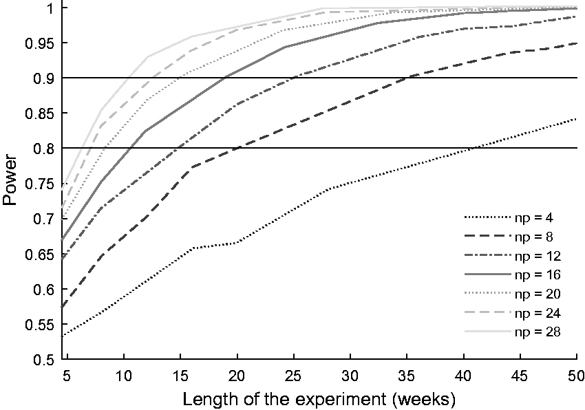

As detailed in Section 2.7, participants and two test environments which met the criteria were found and they had a total number of 46 potential participants. It was expected that around np = 28 will provide usable data (the potential 46 being reduced by absenteeism, unwillingness to participate, forgetting to fill in questionnaires and business travel). With np being 28, a duration of 12 weeks is required to meet the power criteria, which was set at 0.9.

Having a number of participants higher than that required can also help with possible over- or under-dispersion of the data. Over-dispersion is an additional effect that can lower the power of the test in the actual experiment due to the variation between the individual complaint probabilities. In the case of big individual differences, the standard error of the overall complaint probability can be different from the expected one coming from a binomial distribution.

2.2 Environment

Two wings, on two different floors of an office building at the High Tech Campus in Eindhoven, The Netherlands, were selected to carry out the experiment. It was one of the authors’ own buildings; however, the chosen spaces were not. Both spaces were on the south side of the building, next to windows. The space on the second floor was an electronics workbench, shown on the left in Figure 2, the space on the first floor was a typical open office, shown on the right in Figure 2. Typical activities/tasks carried out by the participants in the workbench included the designing, building, measuring and maintaining of electrical components and equipment, and there the LED fixtures together with daylight were the main source of illumination. The employees in the open office carried out typical office tasks, notably working on their laptops, meaning that, in addition to luminaires and daylight, the displays were a source of illumination.

Figure 2

Pictures of the spaces used to carry out the experiment, (left) electronics workbench, (right) open office space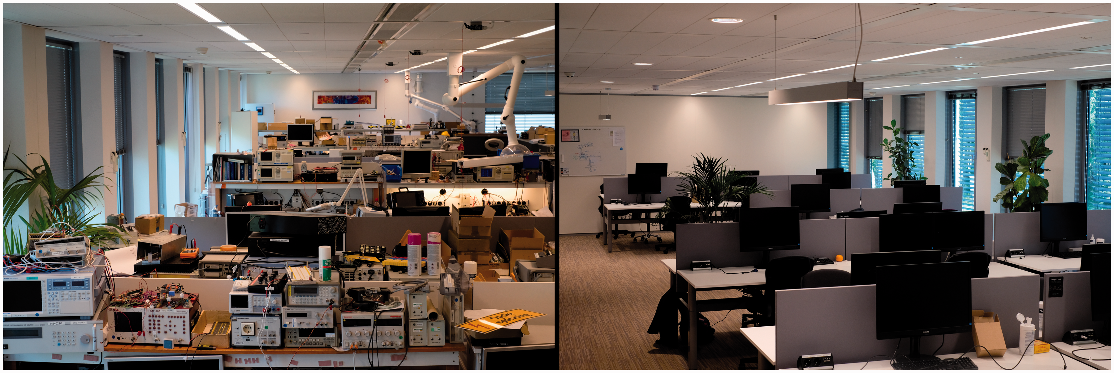

Sixty LED fixtures in the two spaces were equipped with an additional driver, enabling them to switch output. The light settings switched on a weekly or daily basis from the originally installed condition to an intervention by means of an automated timer. Other than the change of the driving current waveform, there was no change in the appearance of the luminaires, the spectrum or the behaviour of the lighting system. The illuminance provided by the electric lighting was fixed at 500 lux on the horizontal working surfaces. This was in addition to any daylight that might be present. All windows were fitted with automatic blinds that limited the amount of direct daylight on the working surfaces.

2.3 Light stimuli

Two lighting stimuli were used in this study, the originally installed condition, referred to as reference and a condition with an increased amount of modulation, referred to as intervention. In Figure 3, their light output as a function of time is shown at the top and their spectral analysis, by means of Fourier transform, at the bottom. Both light waveforms were sinusoidally modulated at the frequency of 100 Hz. The reference had a modulation depth (MD) of 12.5% and a stroboscopic visibility measure (SVM) of 0.47, whereas the intervention had a MD of 36.4% and an SVM of 1.34. SVM = 1 defines the visibility threshold of the stroboscopic effect in a general lighting application. SVM = 1.5 has been proposed as a limit of stroboscopic effect acceptability in a typical office.^23,24 The intervention with SVM = 1.34 has been chosen because such illumination produces visible stroboscopic effect, but it is also considered to be acceptable. The bottom graphs in Figure 3 also show the stroboscopic effect sensitivity curve (dashed), as defined in Perz et al.;²⁵ if the amplitude of a light stimulus with a single frequency component is larger than this curve, the stroboscopic effect produced by this stimulus is visible. This is the case for the intervention light stimulus but not for the reference.

Figure 3

Light stimuli used in the study (left) reference, (right) intervention. The upper graphs depict relative illuminance as a function of time, showing significantly larger modulation depth of the intervention setting as compared to the reference setting. The lower graphs show that both waveforms are modulated at a fundamental frequency of 100 Hz. The stroboscopic effect sensitivity curve (dashed) bounds regions of non-visible (below the curve) and visible (above the curve) effect MD: modulation depth; SVM: stroboscopic visibility measure.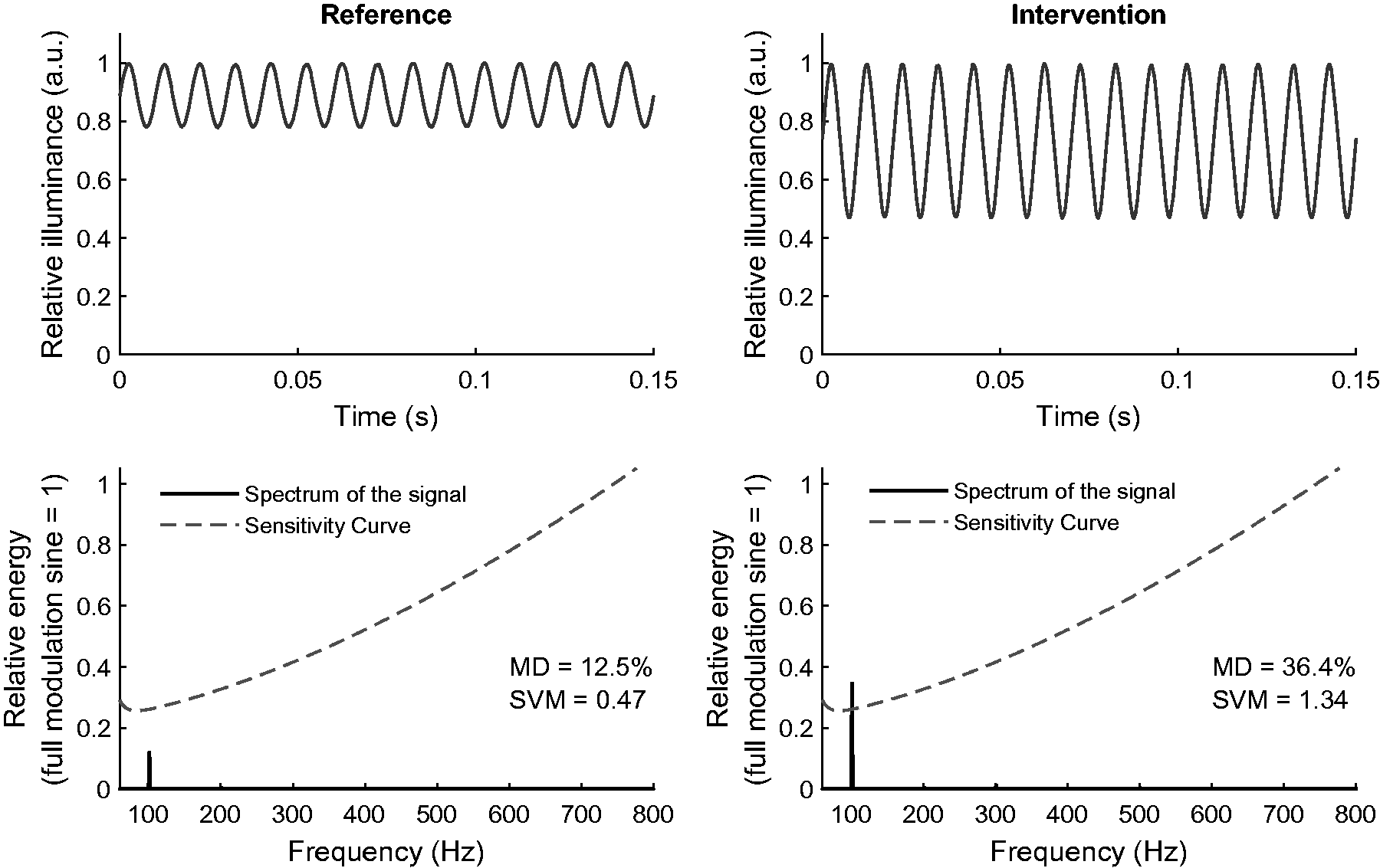

2.4 Daylight analysis

In each space, the desks are arranged in rows of three from the windows (see Figure 2). The amount of daylight contribution to the illumination from LED fixtures (i.e. 500 lux) was measured at each desk, without the blinds. The daily average amount of the total solar radiation incident on a horizontal surface at the surface in front of the building, where the experiment was conducted, was obtained from the NASA Langley Research Center POWER Project.²⁶ The daily profile of global horizontal irradiance was estimated from daily integral and location.²⁷ Then, for every working hour, from 9.00 a.m. until 5.30 p.m., of every day of the experiment, the SVM was computed using the sum of the respective amount of the reference stimuli (SVM = 1.34) and daylight (SVM = 0). Figure 4 shows an example of how the contribution of daylight changed the SVM on three different desks, where Desk 1 is the closest and Desk 3 the furthest from the window. It shows that, as expected, the SVM is highest at the beginning and at the end of the day and the lowest around noon.

Figure 4

The SVM values as a function of the time of the day computed at three desks in the open office, for one day of the experiment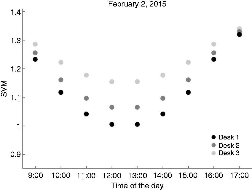

The SVM values were further averaged across all the study days in the two spaces, and Figure 5 shows the results as violin plots, including the minimum, first quartile (Q1), mean and median, third quartile (Q3) and the maximum. The shape of the violin plot shows the distribution of the data. Additionally, the dotted line in Figure 5 depicts the stroboscopic effect visibility threshold, i.e. SVM = 1.

Figure 5

Violin plots of the SVM for time of the day, averaged over all days of the study for (left) electronics workbench and (right) open office. The mean and median values are depicted as a solid and dashed lines, respectively. The borders of the darker shaded areas mark the 25th and 75th percentiles. The dotted line corresponds to the visibility threshold, i.e. SVM = 1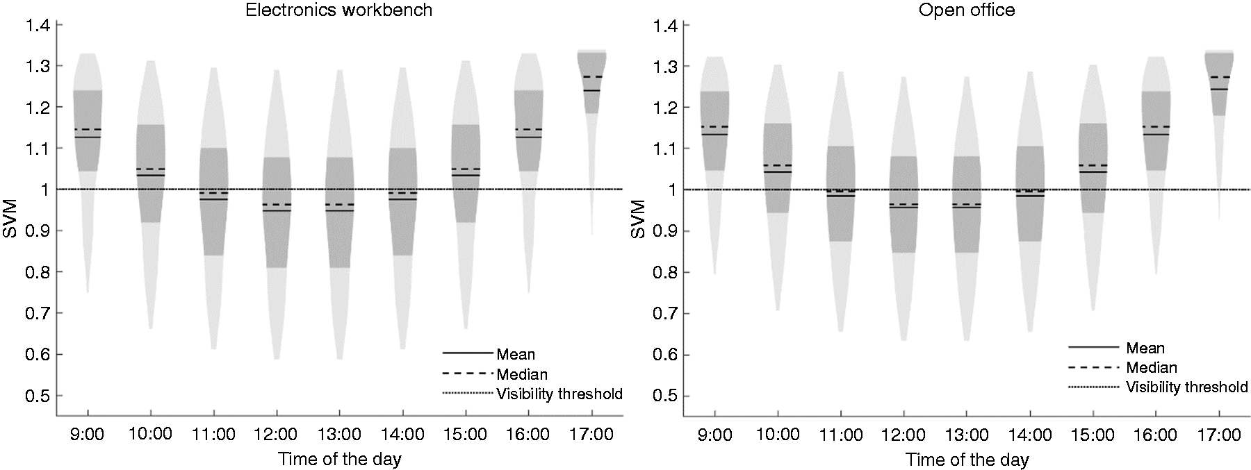

Figure 5 shows that mostly, during the day, the lighting is above the visibility threshold, notably at the beginning and at the end of the day. This was found to provide adequate illumination for the study.

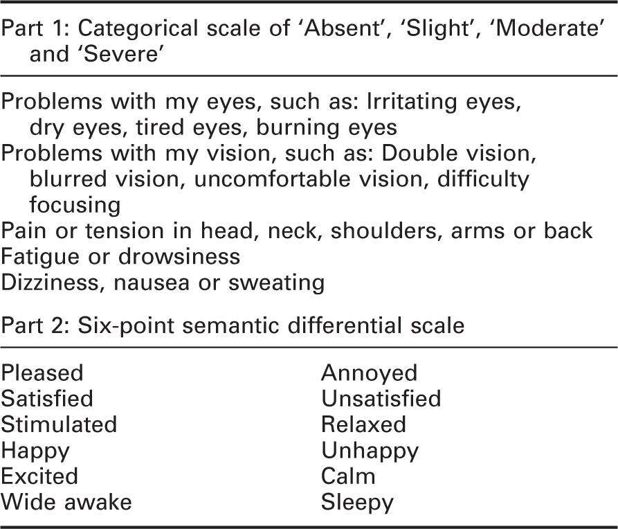
2.5 Questionnaires

To assess the potential detrimental effect of the lighting on the health and wellbeing state of the participants, two sets of questionnaires were used. The first set contained questions related to visual discomfort and other complaints that can result from visual discomfort, depicted in Table 1 on the top. The participants were instructed to rate each of the questions on a four-point categorical scale of ‘Absent’, ‘Slight’, ‘Moderate’ and ‘Severe’. The questions used were inspired by the work of Kennedy et al.²⁸ Additionally, a second set of questions were used to measure the mood of the study participants, using six-point semantic differential scale; the words which were used are given in Table 1, at the bottom. The questionnaire used in this study is shown in Appendix A.

Table 1

Description of the two parts of the questionnaire

Part 1: Categorical scale of ‘Absent’, ‘Slight’, ‘Moderate’ and ‘Severe’
Problems with my eyes, such as: Irritating eyes, dry eyes, tired eyes, burning eyes
Problems with my vision, such as: Double vision, blurred vision, uncomfortable vision, difficulty focusing
Pain or tension in head, neck, shoulders, arms or back
Fatigue or drowsiness
Dizziness, nausea or sweating
Part 2: Six-point semantic differential scale
Pleased	Annoyed
Satisfied	Unsatisfied
Stimulated	Relaxed
Happy	Unhappy
Excited	Calm
Wide awake	Sleepy

2.6 Procedure

On each day of the experiment, the participants received two emails, one at the start of the day and one at the end of the day. Every email had a link to the online questionnaire for the corresponding participant, date and time of day. Participants were not in the building when the light settings switched. Apart from the online questionnaires, the participants did not perform any additional tasks and proceeded with their day-to-day work while immersed in one of the lighting conditions.

The experiment took place during 13 consecutive weeks from January to April. The light conditions were switching between reference and intervention and the schedule of two spaces is given in Table 2. The weeks with the reference settings are marked with ‘off’, while the weeks with the intervention with ‘on’. The weeks marked with ‘mix’ had the setting change every day, with different settings on the different floors. The first four weeks of the study were used to establish a benchmark; due to an unforeseen error, the experimental condition was accidently switched on in the first week in the workbench. After the first four weeks, the settings were switching on a weekly basis, counterbalanced between the two spaces. During weeks 8 and 9, the settings were switched on a daily basis, also counterbalanced between the two spaces.

Table 2

Light setting switching schedule in the two spaces of the experiment

Week no.	1.	2.	3.	4.	5.	6.	7.	8.	9.	10.	11.	12.	13.
Workbench	On	Off	Off	Off	Off	On	Off	Mix	Mix	On	Off	On	Off
Office	Off	Off	Off	Off	On	Off	On	Mix	Mix	Off	On	Off	On

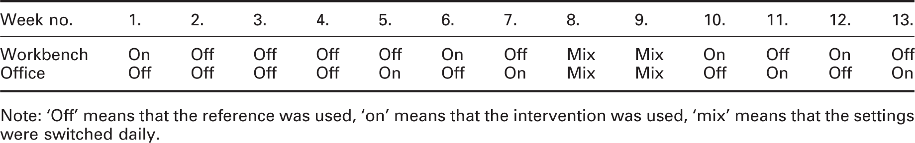
Note: ‘Off’ means that the reference was used, ‘on’ means that the intervention was used, ‘mix’ means that the settings were switched daily.

2.7 Participants

A group of 46 employees of Philips Lighting were exposed to both the reference and the intervention. Twenty-five of these employees worked at the electronics workbench space and 21 in the open office. They were 42 male and 4 female participants, with their age ranging from 36 to 65 years; a detailed distribution of the participants’ age is shown in Figure 6. Most of the participants had general lighting knowledge. They were not informed about the intervention tested in the experiment.

Figure 6

Age distribution of the participants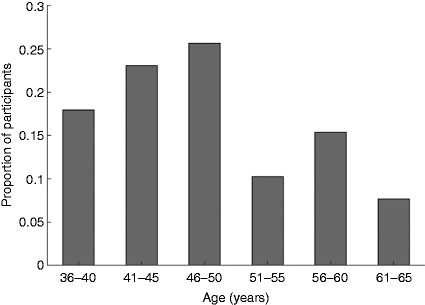

A total of 2813 completed surveys were collected over a period of 13 weeks. Figure 7 depicts the number of surveys competed per day over the experiment period. The participants had the chance to opt out of the experiment at any moment without giving a reason, but none of the participants chose to do so. They were asked to report any serious complaints that they believed were caused by the lighting at which point the experiment would be prematurely stopped. In total, there were 35 participants that filled out more than 20 questionnaires at the start of the day and 24 participants that filled out more than 20 questionnaires at the end of the day.

Figure 7

Questionnaire completion rates over the 13 weeks of the study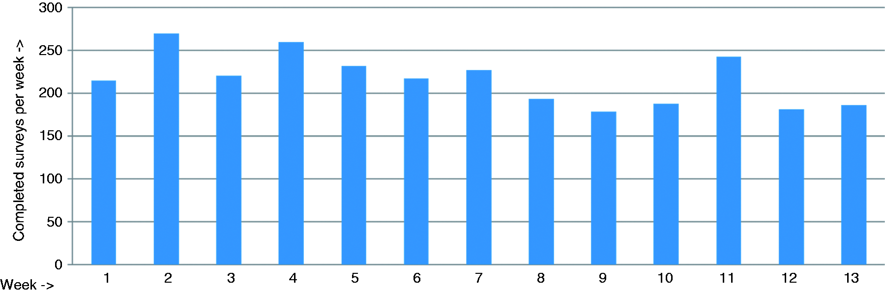

3. Results

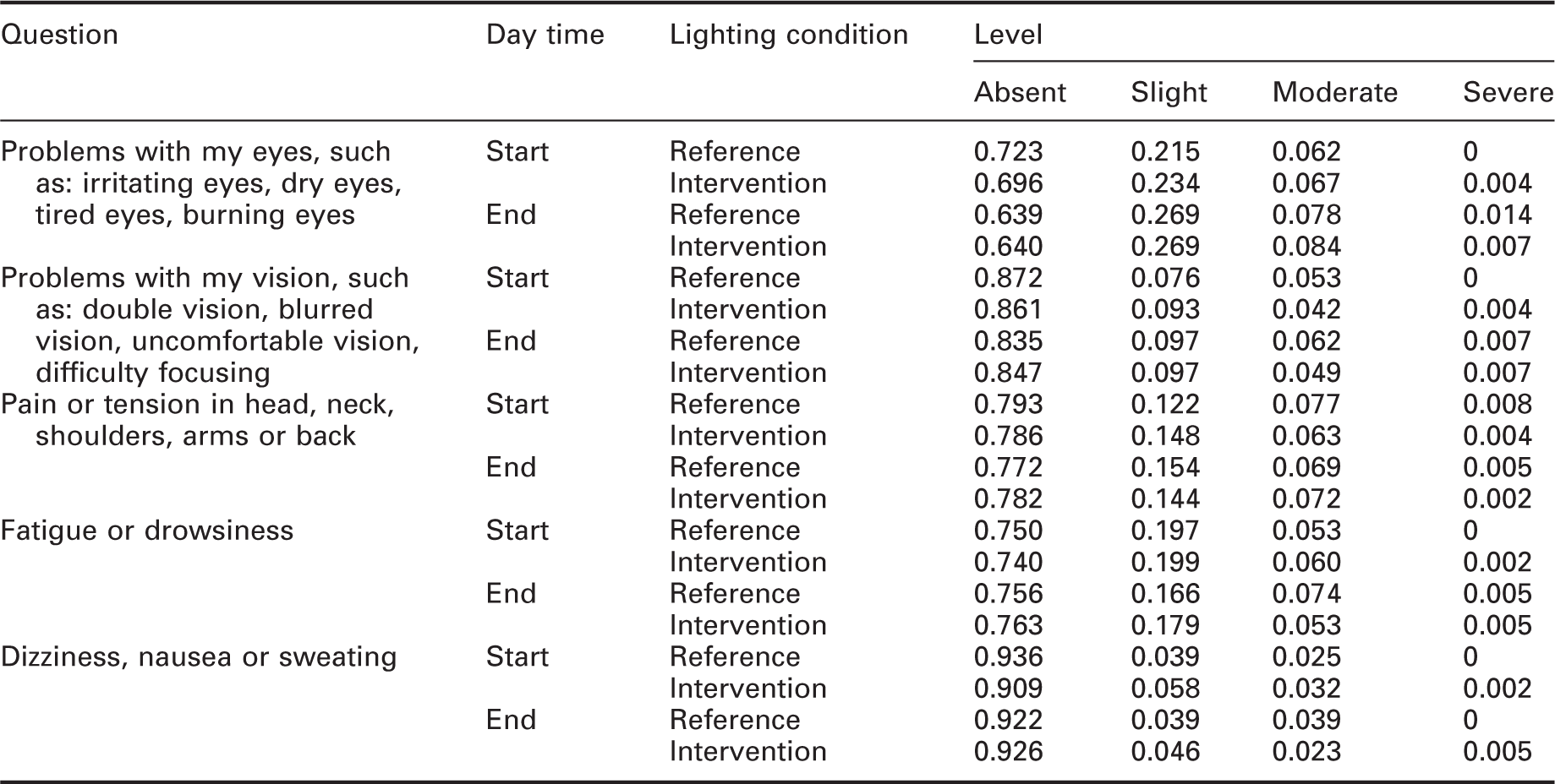
After the end of the experiment, all the results were anonymized and aggregated. Tables 3 and 4 give an overview of the results over all participants for the two parts of the questionnaire.

Table 3

Results for the questions of the first part of the questionnaire, expressed as proportion of each complaint level to the total amount of collected responses

Question	Day time	Lighting condition	Level
			Absent	Slight	Moderate	Severe
Problems with my eyes, such as: irritating eyes, dry eyes, tired eyes, burning eyes	Start	Reference	0.723	0.215	0.062	0
		Intervention	0.696	0.234	0.067	0.004
	End	Reference	0.639	0.269	0.078	0.014
		Intervention	0.640	0.269	0.084	0.007
Problems with my vision, such as: double vision, blurred vision, uncomfortable vision, difficulty focusing	Start	Reference	0.872	0.076	0.053	0
		Intervention	0.861	0.093	0.042	0.004
	End	Reference	0.835	0.097	0.062	0.007
		Intervention	0.847	0.097	0.049	0.007
Pain or tension in head, neck, shoulders, arms or back	Start	Reference	0.793	0.122	0.077	0.008
		Intervention	0.786	0.148	0.063	0.004
	End	Reference	0.772	0.154	0.069	0.005
		Intervention	0.782	0.144	0.072	0.002
Fatigue or drowsiness	Start	Reference	0.750	0.197	0.053	0
		Intervention	0.740	0.199	0.060	0.002
	End	Reference	0.756	0.166	0.074	0.005
		Intervention	0.763	0.179	0.053	0.005
Dizziness, nausea or sweating	Start	Reference	0.936	0.039	0.025	0
		Intervention	0.909	0.058	0.032	0.002
	End	Reference	0.922	0.039	0.039	0
		Intervention	0.926	0.046	0.023	0.005

Table 4

Results for the questions of the second part of the questionnaire, expressed as proportion of each mood level to the total amount of collected responses

Question	Day time	Lighting condition	Level
			3	2	1	−1	−2	−3
Pleased/annoyed	Start	Reference	0.184	0.599	0.131	0.072	0.012	0.002
		Intervention	0.202	0.562	0.130	0.086	0.016	0.004
	End	Reference	0.225	0.543	0.145	0.083	0.005	0
		Intervention	0.218	0.552	0.139	0.084	0.007	0
Satisfied/unsatisfied	Start	Reference	0.212	0.603	0.113	0.062	0.008	0.002
		Intervention	0.236	0.564	0.104	0.079	0.016	0.002
	End	Reference	0.251	0.531	0.136	0.071	0.012	0
		Intervention	0.260	0.552	0.109	0.067	0.012	0
Stimulated/relaxed	Start	Reference	0.145	0.169	0.169	0.161	0.343	0.013
		Intervention	0.158	0.163	0.183	0.135	0.343	0.018
	End	Reference	0.195	0.175	0.161	0.143	0.301	0.025
		Intervention	0.176	0.151	0.165	0.144	0.353	0.012
Happy/unhappy	Start	Reference	0.205	0.586	0.135	0.064	0.007	0.003
		Intervention	0.223	0.566	0.114	0.084	0.011	0.002
	End	Reference	0.235	0.533	0.143	0.083	0.007	0
		Intervention	0.251	0.550	0.123	0.070	0.007	0
Excited/calm	Start	Reference	0.036	0.112	0.246	0.204	0.340	0.062
		Intervention	0.048	0.109	0.236	0.209	0.355	0.044
	End	Reference	0.067	0.124	0.262	0.191	0.306	0.051
		Intervention	0.067	0.095	0.267	0.169	0.350	0.051
Wide awake/sleepy	Start	Reference	0.200	0.514	0.130	0.120	0.035	0.002
		Intervention	0.211	0.519	0.132	0.114	0.023	0.002
	End	Reference	0.320	0.402	0.140	0.115	0.023	0
		Intervention	0.313	0.457	0.128	0.081	0.019	0.002

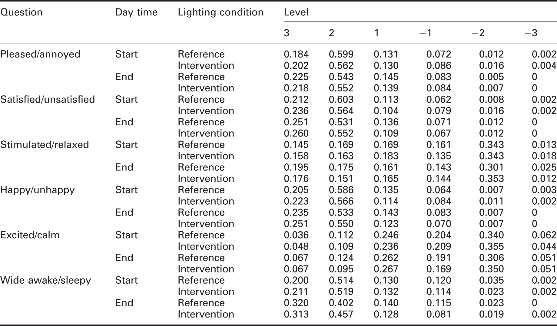
Table 3 shows the responses to the questions from the first part of the questionnaire, expressed as proportion of each complaint level (absent, slight, moderate and severe) to the total number of responses in a given condition. Different numbers of responses were collected for different conditions, being: start of day reference N = 609, start of day intervention N = 569; end of day reference N = 435, end of day intervention N = 431.

Table 3 shows that mostly the complaints in all questions were reported to be absent, notably in the last question over 90% of all the responses reported dizziness, nausea or sweating to be absent. Slight level of problems with eyes (question 1) were reported in different conditions in 21% to 27% of the responses; 17% to 20% reported slight levels of fatigue or drowsiness (question 4) and 13% to 15% reported slight levels of pain or tension in head, neck, shoulders, arms or back (question 3). Responses of moderate complaint level constitute less than 10% and of severe level less than 1% (except question 1, end of the day reference) of all the responses to all the questions.

Table 4 shows the responses to the questions from the second part of the questionnaire, expressed as proportion of each level of a given mood to the total amount of responses in a given condition. The level ranges from 3 to −3, where the positive number corresponds to the first mood describing word (e.g. pleased in question 1) and the negative number to the second word (e.g. annoyed on question 1). Clearly, larger absolute numbers indicate higher association with a given mood (e.g. 3 is more pleased than 2). Similar to the first part of the questionnaire, the total number of collected responses was different across the conditions, as follows: start of day reference N = 609, start of day intervention N = 569; end of day reference N = 435, end of day intervention N = 431.

Table 4 shows that mostly the participants reported to be pleased and not annoyed; combined, levels 1 to 3 amount to 89% to 91% of all the responses. Aggregating the three levels shows that the participants were mostly satisfied, with the responses ranging from 90% to 93%, mostly happy, with 90% to 92%, and mostly wide awake, with 84% to 90%. The responses are roughly evenly distributed between stimulated and relaxed (48% to 53%). Finally, the participants reported to be somewhat calmer (55% to 61%) than excited.

3.1 Data analysis

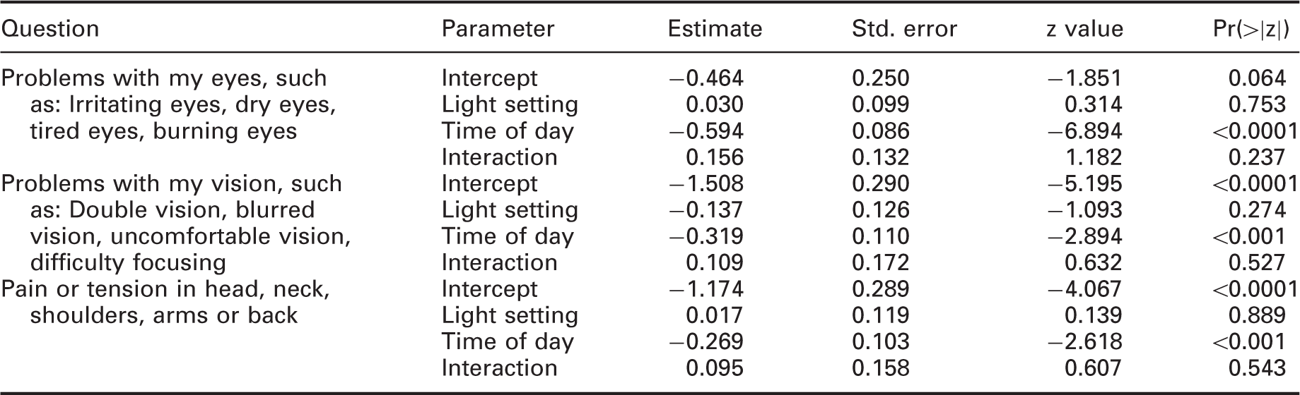
A generalized linear mixed model (GLMM) was fitted to the data using a binomial distribution and a probit link function. For the first part of the questionnaire, all the complaint levels (i.e. slight, moderate and severe) were grouped together resulting in a binary outcome of no complaints, and slight or more severe complaints. The time of the day (‘Start’, ‘End’), the light setting (‘Reference’, ‘Intervention’) and the interaction term between them were added as fixed factors to the model. The identification of the participant was added to the model as a random factor contributing a random intercept, i.e. allowing for a different baseline complaint probability per participant. The parameters estimation was based on the maximum likelihood, using Gauss-Hermite quadrature, by means of the statistical package R and the mixed model library lme4.²⁹

Results of the statistical analysis of the first part of the questionnaire show a significant effect of the time of the day for the first three questions (p < 0.001). Table 5 shows parameter estimates and standard errors of the GLMM for these questions. The significance of each parameter was assessed using the Wald statistics. For these questions, the estimate is negative, meaning that the associated complaints are worse at the end of the day, as compared to the start of the day. The time of the day was not significant for the remaining two questions (p = 0.67, p = 0.38). The analysis showed no significant effect of light setting for any of the questions, with the corresponding values of significance being p = 0.75, p = 0.27, p = 0.89, p = 0.67 and p = 0.38. Moreover, no significant interaction between the time of the day and the light setting was found, with the significance values of p = 0.24, p = 0.53, p = 0.54, p = 0.91 and p = 0.32.

Table 5

Parameter estimates with their standard errors and significance values of the GLMM for the first three questions of the first part of the questionnaire

Question	Parameter	Estimate	Std. error	z value	Pr(>\|z\|)
Problems with my eyes, such as: Irritating eyes, dry eyes, tired eyes, burning eyes	Intercept	−0.464	0.250	−1.851	0.064
	Light setting	0.030	0.099	0.314	0.753
	Time of day	−0.594	0.086	−6.894	<0.0001
	Interaction	0.156	0.132	1.182	0.237
Problems with my vision, such as: Double vision, blurred vision, uncomfortable vision, difficulty focusing	Intercept	−1.508	0.290	−5.195	<0.0001
	Light setting	−0.137	0.126	−1.093	0.274
	Time of day	−0.319	0.110	−2.894	<0.001
	Interaction	0.109	0.172	0.632	0.527
Pain or tension in head, neck, shoulders, arms or back	Intercept	−1.174	0.289	−4.067	<0.0001
	Light setting	0.017	0.119	0.139	0.889
	Time of day	−0.269	0.103	−2.618	<0.001
	Interaction	0.095	0.158	0.607	0.543

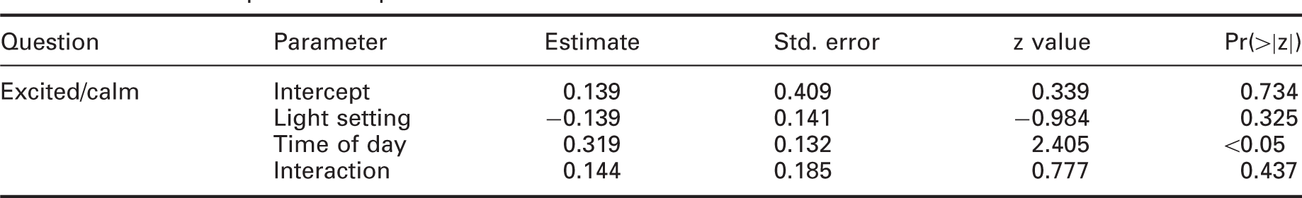
The data of the second part of the questionnaire were also binarized before fitting a generalized linear mixed model. This could be done in a natural way as the number of possible answers was even (from −3 to 3), and there was no neutral number. As in the GLMM in the first part, the time of the day, the light setting and the interaction term between them were added as fixed factors, and the participant was added as a random factor to the model.

Results of the statistical analysis of the second part of the questionnaire show a significant effect of the time of the day for one question (i.e. excited/calm). Table 6 shows parameter estimates and standard errors of the GLMM for this question. The estimate is positive meaning that the respondents were on average calmer at the end of the day. No other significant effects were found, with the significance values of time of the day for the remaining questions ranging from 0.26 to 0.73, of the light setting from 0.17 to 0.81, and of the interaction from 0.27 to 0.82.

Table 6

Parameter estimates with their standard errors and significance values of the GLMM for the question: calm/excited of the second part of the questionnaire

Question	Parameter	Estimate	Std. error	z value	Pr(>\|z\|)
Excited/calm	Intercept	0.139	0.409	0.339	0.734
	Light setting	−0.139	0.141	−0.984	0.325
	Time of day	0.319	0.132	2.405	<0.05
	Interaction	0.144	0.185	0.777	0.437

4. Discussion and conclusion

Even though no statistically significant effect of the light setting was found, several other interesting statistically significant effects were found. The number of complaints significantly increased during the day for the questions with a significant effect of time of day. As no interaction effect was found, the increase of complaints was equal for both light settings. Another time effect was found over the whole duration of the experiment. The number of complaints significantly decreased, and the mood became more positive with time, easily explainable by the transition from winter to spring.

From the demographics, a significant effect of age was found. The biggest effect of age on visual discomfort was between the groups above 50 and below 50 years of age. Upon comparing these groups, there was a significant difference in: Probability of eye and vision problems start and end of day; headache probability at the end of the day and fatigue at the end of the day. In all cases, the above 50 group had increased probability of complaints. The increased probability occurred equally both in the reference condition and in the intervention.

To test if the effect of light setting was different for participants with different probability of complaints, the end of day data from the first part of the questionnaire were fit to a GLMM with both a random intercept and slope per participant. While the intercept significantly differed across participants, there was no significant difference in the slopes between participants, indicating no effect of light setting for participants with both low and high probability of complaints.

Lastly, power analysis was carried out using parametric bootstrap of the data. For all the questions in the first part of the experiment, the data for each participant and light setting separately were bootstrapped 10,000 times using the probability of complaints from the data and the number of questionnaires the participant filled in. The data were then aggregated per question, and the bootstrapped distribution of the aggregated probability of complaints computed. Based on the power analysis in the design of the experiment, a power of at least 90% for an effect size of 5% was expected. However, the results of the bootstrapping procedure show an observed power of 95% or more for an effect size of 5% for all the questions. Thus, there is a less than 5% chance that there is an increase of more than 5% in the probability of complaints and the experiment failed to detect it.

The results of the study demonstrate that in a real-world application, low levels of temporal modulation that can still produce visible stroboscopic effect do not significantly increase the probability of complaints. Furthermore, the power analysis shows that if there was a practically significant level of complaints increase, the experiment would have found it with a high probability.

Footnotes

Declaration of conflicting interests

The authors declared no potential conflicts of interest with respect to the research, authorship, and/or publication of this article.

Funding

The authors disclosed receipt of the following financial support for the research, authorship, and/or publication of this article: These data were obtained from the NASA Langley Research Center (LaRC) POWER Project funded through the NASA Earth Science/Applied Science Program.

ORCID iD

D Sekulovski

References

Kelly

. Visual responses to time-dependent stimuli I. Amplitude sensitivity measurements. Journal of the Optical Society of America A 1961; 51: 422–429.

Commission Internationale de l’Eclairage. CIE Publication 006:2016: Visual Aspects of Time-Modulated Lighting Systems – Deﬁnitions and Measurement Models, Vienna: CIE, 2016.

De Tommaso

Ambrosini

Brighina

. Altered processing of sensory stimuli in patients with migraine. Nature Reviews Neurology 2014; 10: 144–144.

Institute of Electrical and Electronics Engineers. IEEE Standard 1789: Recommended Practices for Modulating Current in High-Brightness LEDs for Mitigating Health Risks to Viewers, Piscataway, NJ: IEEE, 2015.

Porciatti

Bonanni

Fiorentini

Guerrini

. Lack of cortical contrast gain control in human photosensitive epilepsy. Nature Neuroscience 2000; 3: 259–259.

Celesia

Brigell

Gunnink

Dang

. Spatial frequency evoked visuograms in multiple sclerosis. Neurology 1992; 42: 1067–1067.

Marx

Bodis-Wollner

Bobak

. Temporal frequency-dependent VEP changes in Parkinson’s disease. Vision Research 1986; 26: 185–193.

Porciatti

di Bartolo

Nardi

Fiorentini

. Responses to chromatic and luminance contrast in glaucoma: a psychophysical and electrophysiological study. Vision Research 1997; 37: 975–1987.

Fujita

Yamasaki

Kamio

Hirose

Tobimatsu

. Parvocellular pathway impairment in autism spectrum disorder: evidence from visual evoked potentials. Research in Autism Spectrum Disorders 2011; 5: 277–285.

10.

Polak

Schmetterer

Riva

. Influence of flicker frequency on flicker-induced changes of retinal vessel diameter. Investigative Ophthalmology and Visual Science 2002; 43: 2721–2726.

11.

West

Boyce

. The effect of flicker on eye movements. Vision Research 1968; 8: 171–192.

12.

Lee

Pokorny

Smith

Martin

Valbergt

. Luminance and chromatic modulation sensitivity of macaque ganglion cells and human observers. Journal of the Optical Society of America A 1990; 7: 2223–2236.

13.

Smith

Pokorny

Lee

Dacey

. Primate horizontal cell dynamics: an analysis of sensitivity regulation in the outer retina. Journal of Neurophysiology 2001; 85: 545–558.

14.

Conlon

Lovegrove

Hine

. The effects of visual discomfort and pattern structure on visual search. Perception 1998; 27: 21–33.

15.

Wilkins

. Visual Stress, Oxford, UK: Oxford University Press, 1995.

16.

Colman

Frankel

Ritvo

Freeman

. The effects of fluorescent and incandescent illumination upon repetitive behaviors in autistic children. Journal of Autism and Childhood Schizophrenia 1976; 6: 157–162.

17.

Fenton

Penney

. The effects of fluorescent and incandescent lighting on the repetitive behaviours of autistic and intellectually handicapped children. Australia and New Zealand Journal of Developmental Disabilities 1985; 11: 137–141.

18.

Wilkins

Nimmo-Smith

Slater

Bedocs

. Fluorescent lighting, headaches and eyestrain. Lighting Research and Technology 1989; 21: 11–18.

19.

Kuller

Laike

. The impact of flicker from fluorescent lighting on well-being, performance and physiological arousal. Ergonomics 1998; 41: 433–447.

20.

Jaen

Sandoval

Colombo

Troscianko

. Office workers visual performance and temporal modulation of fluorescent lighting. Leukos 2005; 1: 27–46.

21.

Veitch

McColl

. Modulation of fluorescent light: flicker rate and light source effects on visual performance and visual comfort. Lighting Research and Technology 1995; 27: 243–256.

22.

Houle

Turner

Houle

Smitherman

Martin

Penzien

Lipton

. Rounding behavior in the reporting of headache frequency complicates headache chronification research. Headache: The Journal of Head and Face Pain 2013; 53: 908–919.

23.

Perz

Vogels

IMLC

Sekulovski

Heynderickx

. Modeling the visibility of the stroboscopic effect occurring in temporally modulated light systems. Lighting Research and Technology 2015; 47: 281–300.

24.

Perz

Sekulovski

Beeckman

. Acceptability Criteria for the Stroboscopic Effect Visibility Measure. CIE 2017 Midterm Meeting “Smarter Lighting for Better Life” , Vienna: CIE, 2017.

25.

Perz

Sekulovski

Vogels

Heynderickx

. Stroboscopic effect: contrast threshold function and dependence on illumination level. Journal of the Optical Society of America A 2018; 35: 309–319.

26.

National Aeronautics and Space Administration. NASA Langley Research Center. POWER project data sets 2019. Retrieved 24 July 2019, from https://power.larc.nasa.gov/

27.

Roderick

. Estimating the diffuse component from daily and monthly measurements of global radiation. Agricultural and Forest Meteorology 1999; 95: 169–185.

28.

Kennedy

Lane

Berbaum

Lilienthal

. Simulator sickness questionnaire: an enhanced method for quantifying simulator sickness. The International Journal of Aviation Psychology 1993; 3: 203–220.

29.

Bates D, Maechler M, Bolker B. lme4: linear mixed-effects models using S4 classes. R package version 0.999375-39; 2011. Retrieved 25 July 2019, from http://cran.r-project.org/web/packages/lme4/index.html.

Effects of long-term exposure to stroboscopic effect from moderate-level modulated light

Abstract

1. Introduction

2. Method

2.1 Design for possible non-significant results

2.2 Environment

2.3 Light stimuli

2.4 Daylight analysis

2.5 Questionnaires

2.6 Procedure

2.7 Participants

3. Results

3.1 Data analysis

4. Discussion and conclusion

Footnotes

Declaration of conflicting interests

Funding

ORCID iD

References