Sage Journals: Discover world-class research

Abstract

The presence of fog leads to an increase in road traffic accidents. An experiment was carried out using a scale model to investigate how the detection of hazards in peripheral vision was affected by changes in luminance (0.1 cd/m² and 1.0 cd/m² road surface luminance), scotopic/photopic (S/P) ratio (0.65 and 1.40) and fog density (none, thin and thick). Two hazards were used, a road surface obstacle and lane change of another vehicle. Increasing luminance, and reducing from thick to thin fog, led to significant increase in detection rate and a reduction in reaction time, for both types of hazard. The effect of a change in S/P ratio was significant only when measuring detection of the surface obstacle using reaction times, under the thick fog, with an increase in S/P ratio leading to a shorter reaction time.

1. Introduction

For drivers of motorised vehicles, the purpose of road lighting is to allow them to proceed safely, specifically to provide visual cues and reveal potential hazards so that safe vehicular operation is possible.¹ Road lighting reveals objects that are beyond the reach of vehicle forward lighting, which can potentially occur frequently at higher speeds.²

Many aspects of visual performance deteriorate under reduced lighting conditions: spatial resolution, contrast discrimination, stereoscopic depth perception, accommodation response and reaction time.³ Reaction time has been proposed as a suitable proxy for measuring visual performance.⁴

Road lighting on main roads typically uses road surface luminances in the range 0.3 cd/m² to 2.0 cd/m².¹ In this range, we expect higher luminances to lead to a lower percentage of misses⁵ and shorter reaction time⁶ when detecting peripheral targets. Under typical road lighting conditions, vision falls into the mesopic region, the region of transition between the photopic and scotopic states, in which there is a gradual change in spectral sensitivity according to dominance of the rods (scotopic) or cones (photopic). This means that the spectral power distribution (SPD) of the light source is expected to affect performance of tasks in peripheral vision. According to the CIE system for mesopic photometry⁷ this effect of SPD is characterised by the S/P ratio – the ratio of scotopic luminance to photopic luminance. Lighting of higher S/P ratio is expected to reduce reaction time to detection of peripheral targets with this effect increasing at lower luminances.⁶

Vision can be impaired by weather conditions such as fog. Fog is a dense cloud of water droplets lying close to the surface of the ground that occurs when the air temperature approaches its dew point. The UK Meteorological Office describes fog as a visibility of less than 1000 m.⁸ Thick fog reduces visibility to less than 200 m.⁹ Photons of light incident on the water droplets of fog are absorbed and scattered.¹⁰ The effect of absorption of light is a reduction in the luminance of a target; the effect of scattering is to create a veil over the target that reduces its contrast against the background. Reductions in luminance and contrast lead to reduced visual performance.¹¹ This is critical for safe driving because a reduction in detection rate or an increase in reaction time may lead to an increase in road traffic collision frequency and/or severity. Reduced visibility due to fog can distort distance cues and this is one of the main explanations given for the behavioural modifications and high accident rate associated with driving in fog.¹² Note however that both the nature of the task and the degree of fog will affect the likely impact, for example lane-keeping ability does not appear to be affected until visibility is reduced to less than 30 m.¹³

Rather than considering individual tasks, what matters to many people is likely to be the overall effect of fog on road traffic accidents. Two studies of road accidents occurring in fog (or smoke) found that fog led to crashes that were more severe and more likely to involve multiple vehicles; that fog crashes were more likely to occur at night without street lighting; and that there is an elevated prevalence of crashes among young drivers and along undivided rural highways.^14,15

This paper reports an experiment carried out to investigate the influence of fog on drivers’ ability to detect hazards and the interaction between fog density, luminance and light SPD. Road lighting would be of benefit during fog if it improves the ability to detect potential hazards, specifically, if it increases the probability of detection and decreases the reaction time for detection.

2. Apparatus

Hazard detection was investigated using a 1:10 scale model simulating a driver’s view of a road. The driver was located in the middle lane of a three-lane carriageway. The road was lit by the driver’s own headlights on a dipped setting (these were switched on for all trials) and by two arrays of LEDs simulating overhead road lighting, of which the luminance and SPD were varied in trials. Two detection tasks were carried out in parallel: detection of a suddenly appearing obstacle in the road ahead, with detection indicated by pressing a foot pedal similar to a braking action, and detection of one or other of the two vehicles ahead moving into the driver’s lane, with detection indicated by pressing a button on the steering wheel. A third task was used to add cognitive load during trials, and to direct attention ahead rather than onto the detection tasks: this required test participants to read out the intermittently appearing digits on a dynamic fixation crosshair. There were three levels of artificially generated fog (none, thin and thick). The effect of changes in lighting and fog were analysed by comparing the frequency of correct detection responses and the reaction times of these responses.

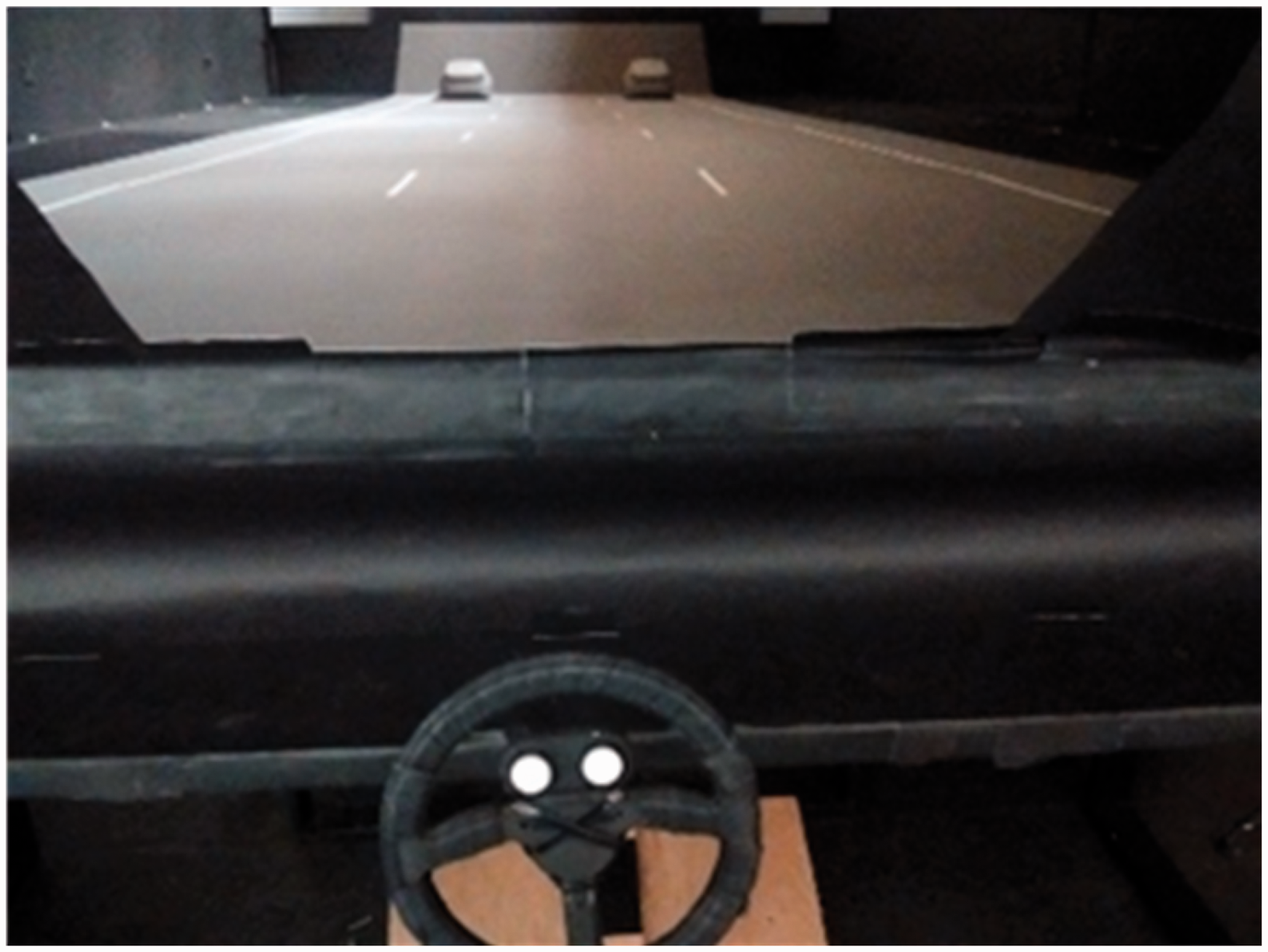
Figure 1 shows the chamber built for this work, a cuboid enclosure of internal dimensions approximately 5 m by 2.5 m by 1.5 m, raised on stilts above the laboratory floor. A driver-participant sitting outside the chamber viewed the interior through an acrylic window at the bottom of one end wall, which put their horizontal sightline approximately 150 mm above the chamber floor. The chamber floor was constructed from MDF sheet painted predominantly in neutral grey (Munsell N5) to represent an asphalt road surface. Other inner surfaces of the chamber (the plywood sidewalls, plywood elements of the ceiling, the end wall with the window) were painted matt-black. The back wall of the chamber was formed by a dark-grey PVC rear-projection screen. Lanes were delineated by continuous and broken white lines applied to the road surface. Test participants sat in a chair adjusted to position their eye level approximately 150 mm above the road surface. There was a response button mounted on a steering wheel beneath the windscreen and a response pedal on an angled footplate on the floor (Figure 2).

Figure 1.

Plan and section through the test chamber including detection targets, overhead road lighting, vehicle forward lighting, viewing position, fog apparatus and fog density lasers.

Figure 2.

The participant’s view of the road ahead, showing the detection-response buttons on the steering wheel.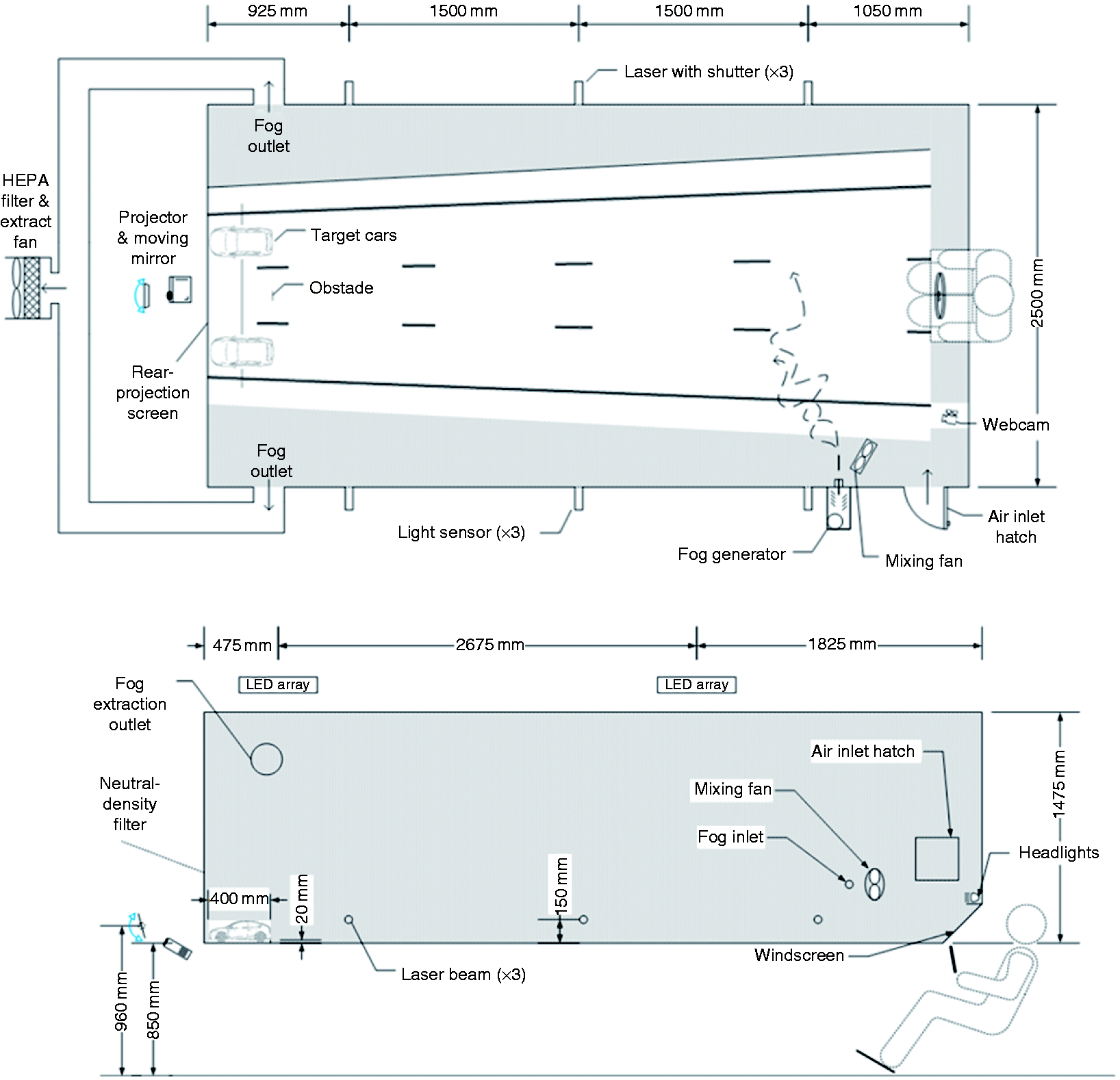

2.1. Lighting

Road lighting inside the chamber was simulated by two LED luminaires located above transparent sections of the ceiling (Figure 1). Each luminaire had six four-colour (red-yellow-green-blue) LED modules arranged in a row, 415 mm long. In front of each module, an acrylic diffuser (opal white Perspex) and small adjustable barn doors (matt-black acrylic) controlled illuminance uniformity and spatial distribution.

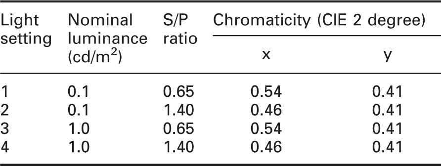
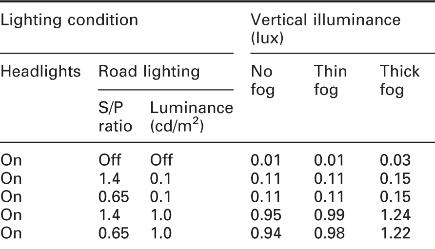
Table 1 shows the light settings used in this work. The luminances were chosen to represent those typical on UK roads¹⁶ with the log unit difference employed with the expectation of revealing a significant effect on detection.¹⁷ Two spectra were chosen, these representing the S/P ratio of high-pressure sodium (HPS, S/P = 0.65) and metal halide (MH, S/P = 1.40) lighting typical of UK roads (Figure 3). Lighting was provided using LEDs to enable rapid switching between settings, significantly reducing experimental time. This simulation means the S/P ratios were matched, but not the precise spectral curves.

Table 1.

Summary of lighting conditions.

Light setting	Nominal luminance (cd/m²)	S/P ratio	Chromaticity (CIE 2 degree)
Light setting	Nominal luminance (cd/m²)	S/P ratio	x	y
1	0.1	0.65	0.54	0.41
2	0.1	1.40	0.46	0.41
3	1.0	0.65	0.54	0.41
4	1.0	1.40	0.46	0.41

Figure 3.

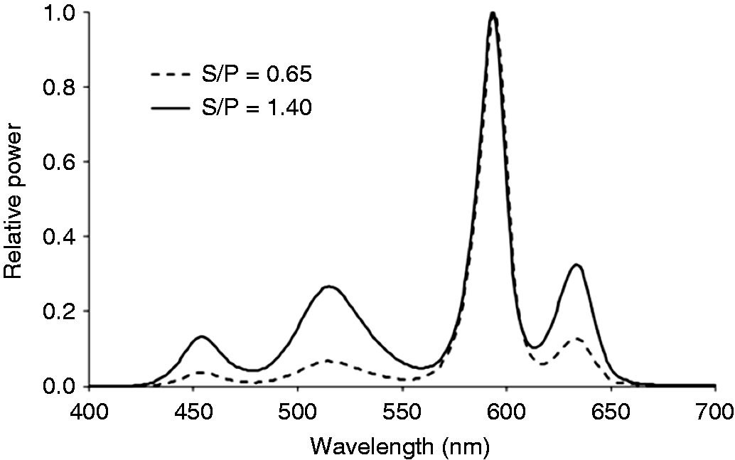
Spectral power distributions (normalised to a peak response of unity) for the two scotopic/photopic (S/P) ratios used in the tests.

Pre-set conditions for the road lighting SPDs and luminances to be tested were established by tuning the four-colour LED intensities by a MATLAB program and confirmed by direct measurement of SPDs inside the chamber (Konica-Minolta CS-1000). During the tests, road lighting was switched between these pre-set conditions by a Python program that also controlled the sequence of detection targets.

Road surface luminance was measured along the centreline of the middle lane with the luminance meter in the location of the test participant as a driver (but without the windscreen). Measurements were recorded at 0.5 m intervals starting at 0.45 m from the far wall (i.e. directly underneath the further LED array). The nominal luminances shown in Table 1 are those at the location of the detection targets. Considering only those luminances measured between the two LED arrays (simulating road lighting at a spacing of 27 m), the mean luminance was 0.87 that of the nominal luminance and with a longitudinal uniformity (minimum/maximum) of 0.58. For the M lighting classes, minimum longitudinal uniformity ranges from 0.4 (M6) to 0.7 (M1).¹⁸

To promote ecological validity, low beam forward lighting from the participant’s vehicle was simulated using two white LEDs (4000 K). Figure 4 shows the SPD. The beam pattern was produced using individual LED lenses and fine-tuned with small adjustable barn doors and opaque masking tape. Beam luminous intensity was controlled with a dimmable constant-current LED driver. The beam pattern was adjusted to give the same relative distribution on the central and adjacent targets as for typical headlamps¹⁹ but with the vertical illuminance lower than typical so that changes in detection were a function of changes in road lighting and not vehicle lighting.

Figure 4.

Spectral power distribution of the driver’s headlight.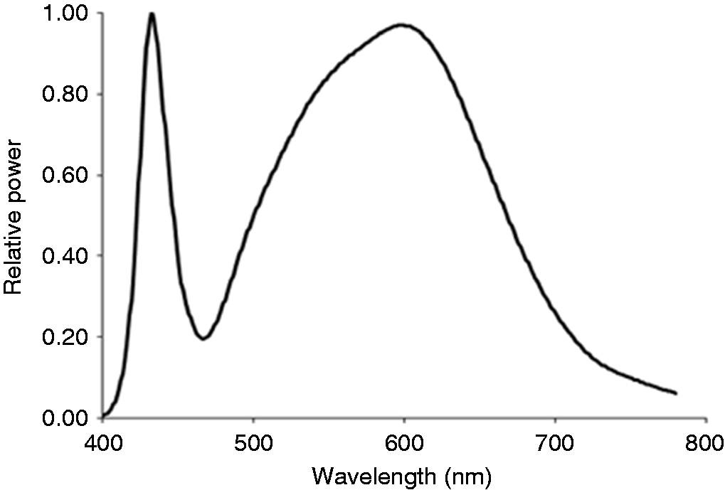

Vertical illuminances from the forward lighting were 0.16 lux at the obstacle and 0.13 lux and 0.17 lux in front of the left-hand and right-hand cars, respectively. This asymmetry is not believed to be significant: analysis of the lane-change detection trials (detection rate and reaction time) did not suggest significant differences between the left-hand and right-hand cars. Considering reaction times to detecting the right and left car lane changes with head-lighting only (these data are reported separately²⁰), which would exaggerate the influence of any asymmetric distribution, did not suggest a significant bias (Mean reaction times for left and right cars were 2731 ms and 2764 ms respectively; p = 0.30, repeated measures t-test, data normally distributed).

The acrylic windscreen had a transmittance uniform across the visible spectrum of approximately 0.9, which is above the minimum required (0.8) for new vehicle windscreens.²¹ Table 2 shows vertical illuminances measured from outside the chamber (i.e. through the windscreen), from the approximate eye position of participants, and aimed towards the target area. These data suggest that thick fog increases illuminance at the eye, as expected due to the increased scatter; that light from the two different SPDs are similarly scattered, which is as expected²²; and that the contribution of the headlamps changes between the two road light luminances, being approximately 10% of illuminance at the eye at 0.1 cd/m² but only 1% at 1.0 cd/m².

Table 2.

Vertical illuminances on the driver’s eyes during trials.

Lighting condition			Vertical illuminance (lux)
Headlights	Road lighting		No fog	Thin fog	Thick fog
Headlights	S/P ratio	Luminance (cd/m²)
On	Off	Off	0.01	0.01	0.03
On	1.4	0.1	0.11	0.11	0.15
On	0.65	0.1	0.11	0.11	0.15
On	1.4	1.0	0.95	0.99	1.24
On	0.65	1.0	0.94	0.98	1.22

2.2. Detection tasks

Test participants were required to detect two events representing drivers situational tasks¹; the appearance of a static obstacle on the road ahead and a car slightly ahead moving into the same lane. In the scale model (Figures 1 and 2) the driver and obstacle were located in the middle lane of a three-lane carriageway while the target cars were located in the nearside and offside lanes, with their unexpected movement into the middle lane being the detection event. All three targets were located 4.7 m ahead of the driver’s eyes and scaled to represent the visual sizes of real targets at 47 m. This distance ahead gave a notional time to impact of approximately 1.5 seconds when driving at 70 mph (113 km/h), which meant the size subtended by the static detection target represented situations where a prompt reaction is necessary to avoid a collision.

The two 1/10th scale cars were body shells (licenced copy of the Ford Focus shape), painted the same neutral grey (Munsell N5) as the road surface and the lower section of back wall to reduce the task contrast (Figure 5). Tail lights were switched off during trials so that detection performance was a function only of changes in road lighting. To enable lane-changing movements, the cars were connected through a slot in the road surface to carriages underneath on a shared linear guide rail. This rail was orientated perpendicular to the run of the road, spanning the three lanes. Each carriage had its own drive system comprising a timing belt, pulleys at the ends of the guide rail, direct drive of one pulley by a stepper motor, an incremental positon sensor (optical encoder) and a proximity sensor to establish absolute position.

Figure 5.

Photographs (from the side, not from the driver’s viewpoint) of the target cars and the raised road obstacle.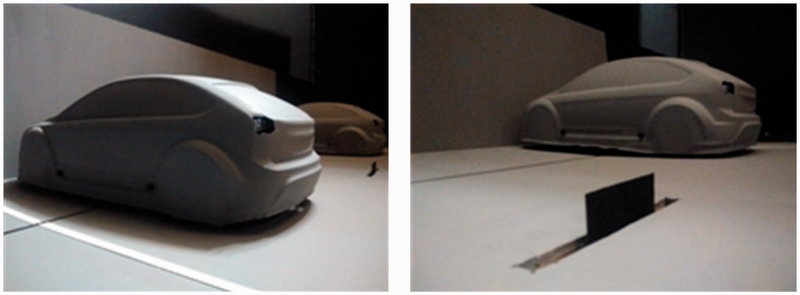

These cars followed two movement patterns: purposeful lane change and random in-lane drift. For the lane changes, motor drives were set to accelerate at 60 mm/s² up to (and down from) a lateral speed of 75 mm/s which completed a move from lane-centre to lane-centre in 6 seconds, simulating the typical speed of a lane change.²³ On arriving at the centre of the middle lane, a car would immediately set off again with the same acceleration and speed settings to return to its home lane. Participants were instructed to press the steering wheel buttons on detecting a lane change. Reaction times were recorded from the onset of a lane-change movement. Responses within 500 ms of the start of a lane change were excluded from the analysis since genuine detection and reaction would likely take longer than this.²⁴ Responses after 6 seconds were assumed to be false alarms (i.e. movement to centre of middle lane complete). Thus, correct detection was assumed to be those events detected between 0.5 seconds and 6 seconds from the onset of a lane change.

In-lane drift usually results from a driver’s imperfect steering inputs. To simulate this, the cars were programmed for a continuous series of lateral moves at speeds between 5 mm/s and 15 mm/s (and acceleration 4 mm/s²) to random positions up to 40 mm either side of the centre of the home lane. Lane changes started from within this range of positions so, for each detected lane change, the recorded data included the particular start position as well as the start time, and the position and time upon detection.

The second detection target represented an obstacle lying in the middle lane, a scaled distance of 47 m ahead of the driver, hence in the same plane as the rear ends of the two cars (Figure 5). The obstacle was formed from a balsawood vane, 60 mm wide and painted matt black to give the appearance of a car tyre lying on its side. This was normally out-of-sight below the surface of the road, but at random intervals could be raised on a servo motor arm through a slot. At its full height of 20 mm the obstacle had the same visual size as a common tyre (e.g. 205/50R16). The obstacle rose to a height of 20 mm in 1 second, remained for 2 seconds, and then took 1 second to drop back out of sight. This rate of growth in visual height is comparable with that of a static obstacle approached when driving. Participants were instructed to press the foot pedal as soon as they noticed the obstacle. Reaction times were recorded from the onset of obstacle movement. Responses in the first 500 ms were excluded from analyses as likely false alarms. Similarly, responses after 4 seconds were ignored as at this point the obstacle would have moved back below the road surface.

A Python program running on a desktop PC coordinated the sequence of obstacles, lane changes and intervals as well as logging reaction times. The reaction time threshold requirements described above resulted in the exclusion of 136 responses, representing 2.9% of all responses made to both detection targets.

Contrasts were calculated as C = (L_t-L_b)/L_b where L_t is the target luminance and L_b is the background luminance.²⁵ The road obstacle was seen in negative contrast, meaning the surface of the vertical target is darker than the road surface it is seen against. For negative contrast, the range of contrasts is 0 to −1.0, with contrasts closer to −1.0 being more visible. Obstacle contrasts were C = −0.88 at 0.1 cd/m², and C = −0.96 at 1.0 cd/m². At the lower luminance, the contribution of the headlamps in lighting the vertical surface of the target is greater than at the higher luminance, which slightly reduces the contrast.

The aspects of the target vehicles that were visible to the test participant presented complex surfaces with three distinct regions – the bumper, tailgate and rear window; all painted matt grey. The luminance of the sloping window was higher than that of the near-vertical bumper and tailgate. Note also that from the driver’s viewpoint, the bumper was surrounded by horizontal road surface, but the tailgate and window were seen against the rear vertical surface (Figure 5). The bumper presented a contrast of approximately C = −0.80 against the road surface, that is a negative contrast. The tailgate presented a positive contrast of approximately C = 0.7 against the side surrounds. Note that the range for positive contrasts extends from 0 to infinity, with higher contrasts being more visible. The window contrast changed with luminance, being approximately C = 8.0 at 0.1 cd/m² and C = 12.0 at the higher luminance. The window to tailgate contrast was approximately C = 6.5.

A dynamic fixation task was used to place the detection tasks, performed in parallel, in the test participant’s peripheral visual field.²⁶ Rather than the static fixation point used in many studies, a dynamic fixation mark simulates the non-static gaze patterns of a driver. The participant was required to track the moving image of a cross projected onto the back wall of the chamber. At irregular intervals between 1 seconds and 6 seconds, the cross would be replaced for 300 milliseconds by a random number between 1 and 9. Participants read aloud the numbers, and the experimenter recorded these responses; the accuracy of identifying these digits was used as a measure of the degree to which fixation was maintained. The cross had a luminance of 1.3 cd/m² against the background luminance of 0.03 cd/m², as measured using a Konika-Minolta LS-110 luminance meter with no other light sources present. It subtended a visual size of 34 minute arc to 54 minute arc at the viewing distance of approximately 5.1 m.

Eye tracking has demonstrated a tendency for driver’s gaze on main roads to fall within a 10° circle.²⁷ The fixation target, therefore, followed a random path within a 10° circle, with the lower fifth excluded to avoid it coming too close to the cars and obstacle: the target was between 6° and 12° above the horizontal sightline and the detection tasks (cars and obstacle) were between 0° and 2° below the horizontal.

Fog would have disrupted a projector beam inside the chamber so the back wall was formed by a rear-projection screen (Rosco Black 2107) and the projector was located outside the chamber. A problem found in projecting a continuously tracking fixation task in dark surroundings is the significant amount of light contained in the black background. To avoid this, the projector was turned away from the screen towards a mirror of the same size as the fixation character. Unwanted background light was absorbed in black fabric surrounding the mirror while the character was reflected onto the screen. The mirror was mounted on a programmable robotic gimbal as in previous work^26,28 enabling movement of the fixation image across the screen.

2.3. Fog simulation

Simulating fog required an artificial fog generator, a mixing fan, an extract system and three lasers for measuring light attenuation to establish different levels of fog density.

The artificial fog, a colourless aerosol of liquid droplets suspended in air, was generated from a mixture of glycerol and water, vaporised in a heat exchanger (Mini Colt 4, Concept Engineering Ltd.). A push-button on the fog generator let the experimenter introduce short bursts of fog directly into the chamber, using the air stream from a mixing fan inside the chamber to disperse the fog. Fog density was reduced (or eliminated completely) using a centrifugal fan unit with a HEPA filter connected to two outlet ducts at the far end of the chamber.

Fog consists of small water droplets: the diameters are suggested to be in the range of 5 µm to 35 µm,¹⁰ although some measurements suggest sizes less than 2 µm make a large contribution.²⁹ The water droplets created in this apparatus were slightly smaller, with a median diameter of 0.2 µm to 0.3 µm. Droplet size matters because it affects how light is scattered, and hence how well it simulates the effect of fog on scattering which is largely insensitive to wavelength.²² For larger droplets, Mie scattering is predominant which is not significantly affected by wavelength, but for smaller droplets then Rayleigh scattering becomes more significant, and this is affected by wavelength.³⁰ Mie scattering is expected when droplet radius (here the smaller median droplet size has radius 0.1 µm) is greater than 0.1 times the wavelength of light (here 0.07 µm for long wavelength light at 700 nm)³¹: this suggests the droplets used in this fog simulation adequately represent the light scatter of real fog. Rayleigh scattering has a stronger effect on light in the short wavelength region, and hence if significant in the current apparatus it would change the S/P ratio. To examine this, the spectra of light reaching the observers were measured, for the two SPDs used in the experiment. For the thick fog (absorption coefficient 0.04 – see below) the S/P ratios decreased by less than 5% compared with that measured with no fog (4.4% for the low S/P ratio lighting and 4.8% for the high S/P ratio lighting).

Fog density was measured by the absorption coefficient of the chamber atmosphere calculated from the attenuation of light propagating through it, the approach used in previous work investigating smoke.³² Light attenuation was measured using the beams from three collimated laser diodes (532 nm, 5 mW, Thorlabs Ltd.) which crossed the chamber 150 mm above the road surface at three locations along the length of the road, this being approximately the eye-height of participants viewing the chamber (Figure 1). Three lasers and sensors were used in order to assess the variation in fog density at different locations in the chamber.

The 3.5 mm-diameter laser beams passed through separate 10 mm diameter windows perpendicularly opposite the lasers to enter the sensor housings outside the chamber. Inside each housing, the sensor (TSL2561, TAOS, Inc.) was located behind a small acrylic diffuser (opal white Perspex) at the end of a 10 mm diameter, 30 mm long tube. The diffuser was expected to reduce the effect of tiny changes in beam-sensor alignment (the two had similar diameters) that might occur during a test session. The tube was included to impede non-laser light paths.

A laptop PC logged the three laser intensities every 2 seconds and displayed the resulting absorption coefficient in numeric and graphical form, allowing the experimenter to monitor fog density. To promote stable measurements, the lasers were powered from a regulated linear supply and kept switched-on from 1 hour in advance of each experiment session.

Two different SPDs were used in these trials, representing the S/P ratios of HPS and a typical MH lamp. These spectra were used to check for possible effects on peripheral detection.^28,33 It is not expected that fog would scatter lighting of different SPDs in different ways since the mean size of water droplets which form fog is usually quite large and theoretically should be the same scatter level for all wavelengths.^34,35

Fog density is defined by the degree to which light is attenuated due to scatter and absorption, and this can be related to visibility distance. The quantitative measure used is the absorption coefficient per unit depth of fog, for which typical values are 0.003 m⁻¹ (light fog), 0.006 m⁻¹ (medium fog) and 0.03 m⁻¹ (heavy fog).¹⁰

Three levels of fog were used in the current work: none, thin and thick (Table 3). The no-fog condition gives a benchmark against which to compare results gained with fog. Thin and thick fog levels were chosen to give a wide difference, and hence it was expected that tests in these conditions would lead to different levels of visual performance. The two fog densities were thick fog with an absorption coefficient of 0.04 m⁻¹, and thin fog with an absorption coefficient of 0.005 m⁻¹. The corresponding percent reductions in measured laser intensity for these conditions, in turn, are 63.2% and 11.7%. The fog densities of the current work represent visibility distances of approximately 600 m (thin fog) and 75 m (thick fog).³⁶ It is very rare to observe fog with a meteorological visibility distance lower than 50 m.³⁶

Table 3.

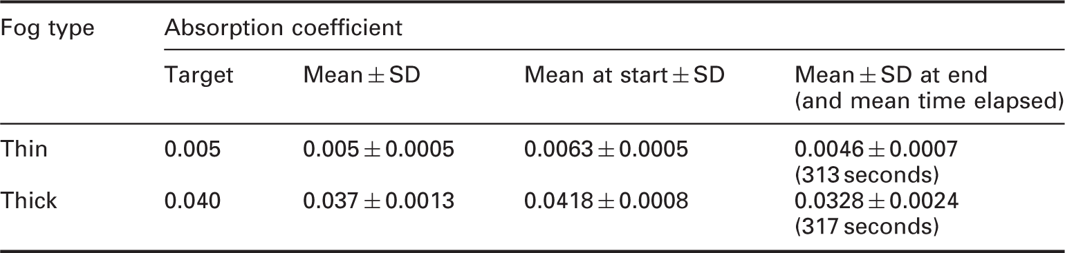
Target and measured levels of fog absorption coefficient as measured immediately before and after each trial.

Fog type	Absorption coefficient
Fog type	Target	Mean ± SD	Mean at start ± SD	Mean ± SD at end (and mean time elapsed)
Thin	0.005	0.005 ± 0.0005	0.0063 ± 0.0005	0.0046 ± 0.0007 (313 seconds)
Thick	0.040	0.037 ± 0.0013	0.0418 ± 0.0008	0.0328 ± 0.0024 (317 seconds)

The visible laser light would confound test conditions during trials, and so fog density was measured immediately before and after trials but not during trials. This was done using remotely controlled motorised shutters on the laser housings. Measurement and logging paused automatically when the experimenter opened the laser shutters, restarting when the shutters were closed.

It was anticipated that the level of fog would slightly decay during trials. Therefore, before each trial, the experimenter increased the level of fog to produce an absorption coefficient slightly above the target (Table 3). Laser shutters were closed immediately before a trial, and immediately after completion of one light-setting trial (4-minute block), they were reopened to check and re-set the level of fog before continuing with trials at the next light condition.

3. Procedure

Participants were seated at the apparatus, ensuring the foot pedal and steering wheel button positions were comfortable before ambient room lights were switched off and a 20-minute adaptation period commenced. During adaptation, with all room lighting switched off and the apparatus lighting was set to the condition the participant would first experience, the experimenter explained the set-up. Participants were instructed to pay attention primarily to the dynamic fixation marker whilst simultaneously responding to the lane change and obstacle detection. They were asked to press the relevant response button/pedal when a detection event was noted, even if not completely sure that it was an event. A practice trial (3 minutes) was carried out to gain familiarity with the stimuli and response mechanisms.

In trials there were three parallel tasks: (i) reading aloud the dynamic fixation digit when this momentarily changed from a crosshair; (ii) pressing the steering wheel button in response to a lane change of one the cars ahead; and (iii) pressing the foot pedal in response to a suddenly appearing road surface obstacle. To notify the participant that their response was acknowledged, it generated an electronic bleep. A recording of ambient sound inside a moving car was played throughout all conditions. Any number called out by the participant in response to the dynamic fixation target was recorded in a spreadsheet by the experimenter.

Presentation orders of the three detection targets (obstacle and two cars) were divided into 1-minute bins. Within each bin, there were four detection events, presentation of two lane changes (either car) and two surface obstacles. These were initiated at pseudo-random intervals randomly selected from between 5 seconds and 26 seconds whilst ensuring that four events were completed in any 1-minute period. No two events overlapped. The number of lane changes was balanced between the cars every two bins, so there were always two right, and two left car lane changes every two bins.

The experiments examined four light settings (Table 1) and three levels of fog. All four light settings were experienced within one block of trials of constant fog level. Within each block, the light setting orders were randomised. The no-fog block was always used first, followed by the thin or thick fog in a counterbalanced order, avoiding the long period required to completely evacuate the chamber of fog. Each trial lasted for 4 minutes and was followed by 1 minute for the experimenter to change the light setting. The tests were completed within a single test session, lasting just under 2 hours.

A sample of 30 test participants was recruited, drawn from two age ranges (younger: 18–30 years and older: 40–70 years) to allow an analysis of the effect of age (Table 4). Acuity was tested using a Landolt ring chart; participants wore corrective lenses for the acuity test and for the test trials if they usually did so when driving. For driving in the UK, drivers are required to be able to read a vehicle number plate at a distance of 20 m, which is a Snellen acuity of approximately 6/10 or better (equivalent to logMAR ≥ 0.20). Of the 30 test participants recruited, all but one were found to have visual acuity at this level or better, this one person being a member of the older sample. The results for this person were retained during analysis: the results (below) show the two minor changes to conclusions that would arise if these data were omitted. Colour vision examined using the Ishihara test (under a D65 source) did not suggest any test participants to have non-normal colour vision. Test participants were given a small reimbursement for their participation.

Table 4.

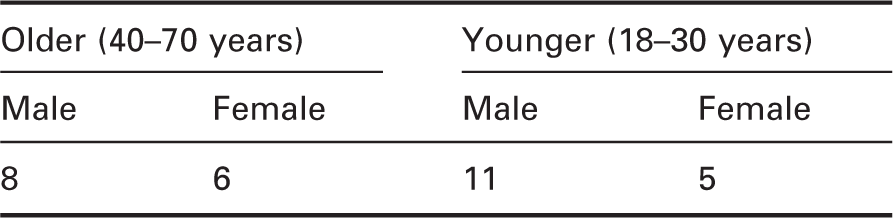
Age and gender breakdown of the test sample.

Older (40–70 years)		Younger (18–30 years)
Male	Female	Male	Female
8	6	11	5

4. Results and analysis

The mean rate of correct identification of the fixation target was 93.6% (SD = 4.6%) during trials with no fog and 93.4% (SD = 5.5%) during trials with thin fog. However, the rate dropped to 80.7% (SD = 12.5%) during trials with thick fog. This decrease in the identification of the fixation target is expected, as the visibility of this target was reduced due to the increase in fog density. These high success rates suggest the fixation target was effectively holding the foveal gaze of participants, ensuring the lane change and obstacle detection tasks were carried out using peripheral vision, as was intended.

Mean detection rates and reaction times were calculated for each of the car and obstacle targets, under each fog and light condition. The experiment had a 2 × 2 × 2 × 3 factorial design. The age group of the participant was a between-subjects factor with two levels (young and old). The luminance of the light condition was a within-subjects factor with two levels (0.1 cd/m² and 1.0 cd/m²). The spectrum of the light condition was also a within-subjects factor with two levels, characterised as low and high S/P ratios. The fog condition was a within-subjects factor with three levels (none, thin and thick). Note that in thick fog the obstacle detection events were detected by only about 40% of the sample at 0.1 cd/m² and 75% at 1.0 cd/m², and hence there was a reduction in the number of reaction time data points under these conditions.

Linear mixed-effects models were used to compare performance between the different conditions, for each combination of target type (car and obstacle) and response type (detection rate and reaction time). This statistical test avoids the need to exclude unmatched data in the within-subjects factors. The distribution of the residuals for each of these models was assessed for normality by examining histogram and QQ plots. Three of the four sets of residuals adequately matched a normal distribution. The model residuals for detection rates of the car target marginally deviated from normality. However, linear mixed-effects models are robust to small deviations from normality (e.g. Warrington et al.³⁷) and use of the model was therefore considered acceptable. Table 5 shows the results from each of these linear mixed-effects models.

Table 5.

F statistics and p-values for detection rates and reaction times to each target. Results based on linear mixed models.

Effect	Car lane change				Obstacle
	Detection rate		Reaction time		Detection rate		Reaction time
	F	p	F	p	F	p	F	p
Age	0.72	0.40	0.98	0.33	2.33	0.14	0.42	0.52
Luminance	9.87	<0.01*	168.1	<0.01*	71.60	<0.01*	39.60	<0.01*
S/P ratio	1.26	0.27	0.86	0.36	0.72	0.40	2.78	0.10
Fog level	35.28	<0.01*	236.8	<0.01*	181.9	<0.01*	37.02	<0.01*
Age × luminance	0.48	0.49	0.76	0.39	1.31	0.26	2.38	0.13
Age × S/P	0.20	0.66	0.28	0.60	0.00	0.95	0.13	0.72
Luminance × S/P	0.06	0.81	0.33	0.57	0.50	0.48	0.09	0.77
Age × fog	0.19	0.82	0.02	0.98	0.26	0.77	0.40	0.67
Luminance × fog	11.81	<0.01*	24.14	<0.01*	8.97	<0.01*	2.17	0.12
S/P × fog	1.16	0.31	0.57	0.57	2.05	0.13	5.73	<0.01*
Age × luminance × S/P	1.99	0.16	0.70	0.41	0.39	0.54	2.04	0.16
Age × luminance × fog	0.10	0.91	0.87	0.42	1.64	0.20	1.48	0.23
Age × S/P × fog	1.01	0.37	1.26	0.29	0.29	0.75	0.47	0.63
Luminance × S/P × fog	0.62	0.54	0.13	0.88	0.82	0.44	0.37	0.69
Age × luminance × S/P × fog	0.74	0.48	0.05	0.95	0.92	0.40	0.13	0.88

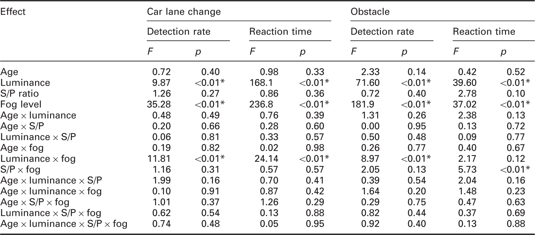
Statistically significant at p < 0.01.

Figure 6 plots the mean detection rates for the lane change by the two age groups and for each combination of fog and light condition. Detection rates for the car were high, reaching near maximal performance under the no fog and thin fog conditions for all light conditions. They were slightly lower when the fog was thick. There also appeared to be a difference in detection rates between the two luminances, with slightly better performance at 1.0 cd/m² compared with 0.1 cd/m². There does not appear to be a consistent and obvious effect of the spectrum, however, nor the age group of the observer.

Figure 6.

Mean detection rates for car lane change by age group, fog condition and light condition. Error bars show the standard error of the mean.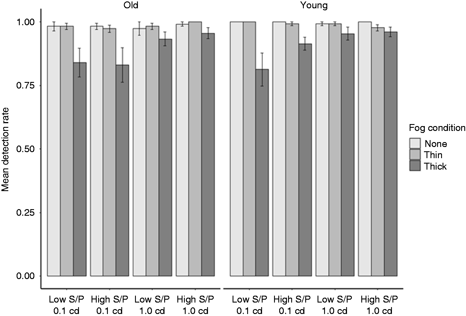

The only statistically significant main effects revealed by the linear mixed-effects model were for luminance and for the fog level. Detection rates were slightly higher at 1.0 cd/m² (mean = 0.98) compared with 0.1 cd/m² (mean = 0.94). A post hoc Tukey test showed that the thick fog condition produced a significantly lower detection rate (mean = 0.90) than both no fog and thin fog conditions (mean = 0.99 for both). There was no difference between the no fog and thin fog conditions. The only significant interaction between the different factors revealed by the linear mixed-effects model was between luminance and fog condition (F(2, 223) = 11.8, p < 0.001). The interaction between luminance and fog condition is plotted in Figure 7. This suggests the increase in luminance made a larger improvement to detection of the car lane changes in the thick fog condition compared with the other two conditions. This was confirmed with post hoc Tukey tests which showed that the change in detection rates between the two luminance levels was not significant for the no fog and thin fog conditions (p = 1.0 for both), but was significant for the thick fog condition (p < 0.001).

Figure 7.

Mean detection rates for car lane change by luminance and fog condition. Error bars show standard error of the mean.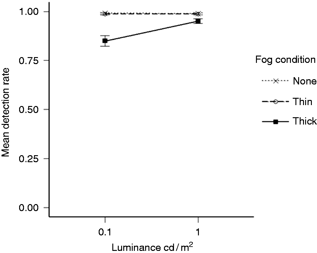

The sample used in these trials included one older driver whose vision, according to the Landolt ring acuity test, does not meet the standard required for driving. The results for this participant have been retained in all analyses reported here. Separate analysis of the data revealed that only two conclusions would change if this participant were removed, and these both relate to detection rates of the car lane change: (i) interaction between fog level and luminance is no longer suggested to be statistically significant and (ii) interaction between SPD and fog becomes statistically significant (p < 0.01).

Figure 8 plots the mean detection rates for the obstacle by the two age groups and for each combination of fog and light condition. The obstacle was detected less often than the car lane change, as this was a more difficult task due to the size and duration of the target. There is again a clear drop in detection rates for the thick fog condition compared with the other two fog conditions. There is also a suggestion that the older age group may have had slightly poorer performance than the younger age group.

Figure 8.

Mean detection rates for obstacle by age group, fog condition and light condition. Error bars show standard error of the mean.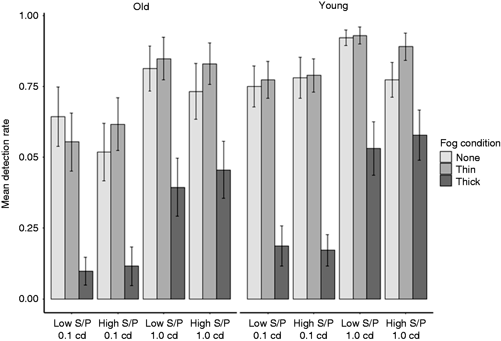

The linear mixed-effects model only found significant main effects for luminance and fog condition. Detection of the obstacle was significantly higher at 1.0 cd/m² (mean = 0.73) compared with 0.1 cd/m² (mean = 0.50). Post hoc Tukey tests did not reveal differences in detection rates during the no fog (mean = 0.75) and thin fog conditions (mean = 0.78, p = 0.49), but detection rates during the thick fog condition (mean = 0.32) were significantly lower than both no and thin fog conditions (p < 0.001 in both cases). The only significant interaction was between the luminance and fog conditions. The interaction between these two factors, plotted in Figure 9, suggests that although detection rates for the obstacle increased for all three fog conditions when luminance was increased from 0.1 to 1.0 cd/m², the increase was larger during thick fog. This interpretation was confirmed by post hoc Tukey tests. These showed that whilst the change in detection rates between 0.1 cd/m² and 1.0 cd/m² was not significant with no fog (p = 0.10), the change was significant when thin fog was introduced (p = 0.003), and even more significant when thick fog was introduced (p < 0.001).

Figure 9.

Mean detection rates for obstacle by luminance and fog condition. Error bars show standard error of the mean.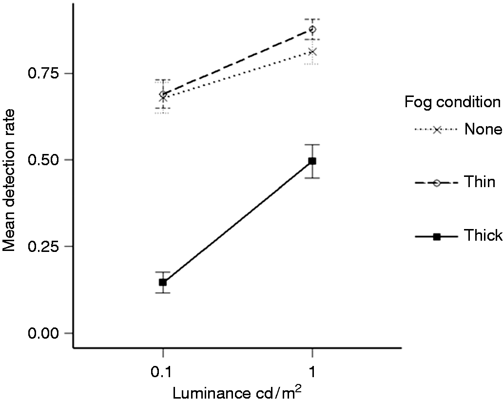

Figure 10 shows the mean reaction times to detection of the car lane change, by age group, light condition and fog condition. There is again a clear difference between reaction times during the thick fog condition compared with the other two fog conditions. There also appears to be an improvement in reaction times when the luminance is increased to 1.0 cd/m², but no obvious difference between the two spectra. There is also no obvious difference in mean reaction times between the two age groups.

Figure 10.

Mean reaction times for detection of car by age group, fog condition and light condition. Error bars show the standard error of the mean.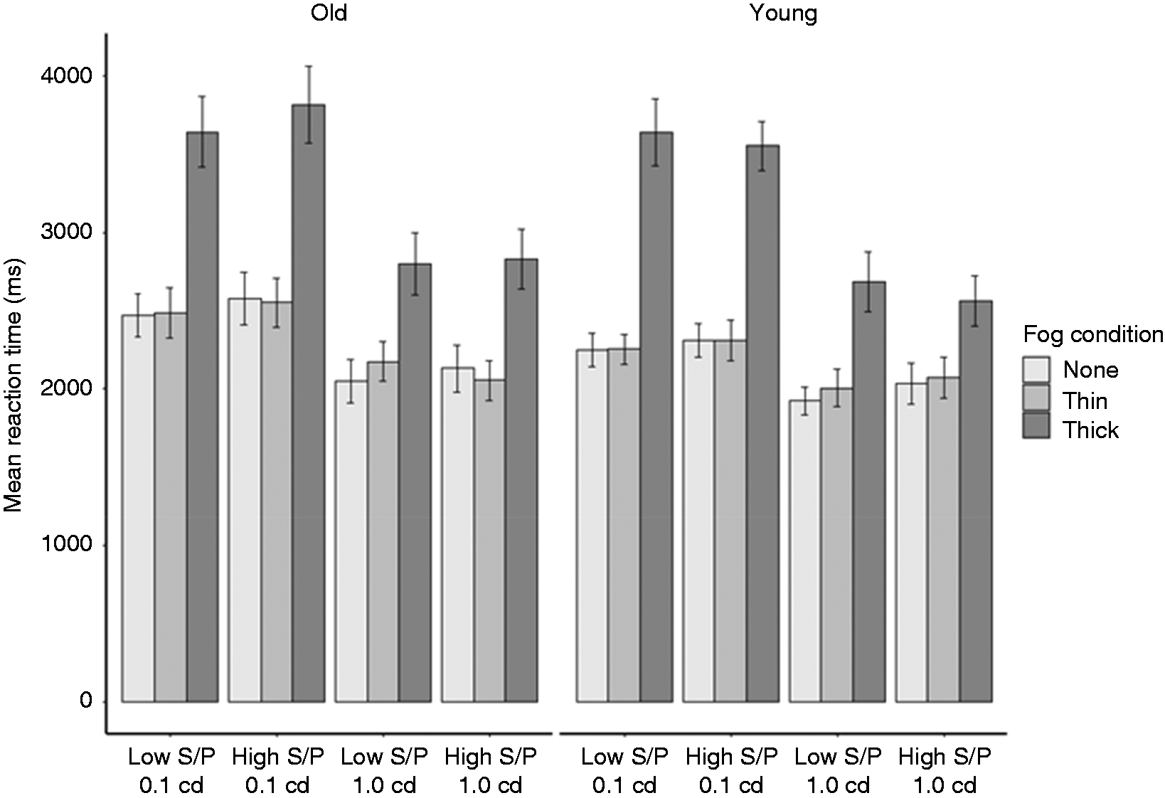

The linear mixed-effects model confirmed that there were significant main effects of luminance and fog condition. The higher luminance produced a significantly shorter reaction time (mean = 2270 ms) than the lower luminance (mean = 2811 ms). Post hoc Tukey tests showed that thick fog produced a significantly slower reaction time (mean = 3187 ms) than both no fog and thin fog conditions (means = 2211 ms and 2234 ms respectively, p < 0.001 in both cases). There was no difference in reaction times between the no fog and thin fog conditions (p = 0.99). The only significant interaction found by the linear mixed-effects model was between luminance and fog condition. This interaction is plotted in Figure 11 and suggests the increase in luminance produced a larger improvement in reaction times during the thick fog condition compared with the other two fog conditions. Post hoc Tukey tests did not confirm this interpretation of the interaction plot, however, as they showed that the increase in luminance significantly reduced reaction times in all three fog conditions (p < 0.005 in all cases).

Figure 11.

Mean reaction times for detection of car by luminance and fog condition. Error bars show the standard error of the mean.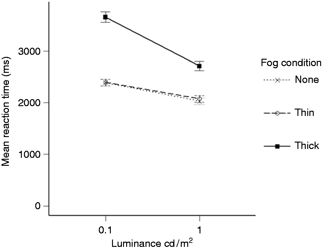

Figure 12 shows the mean reaction time to detection of the obstacle by age group, light condition and fog condition. There are differences in reaction times between the different fog conditions, with slower responses during thick fog and faster responses during no fog. There is no obvious difference between the two age groups, but reaction times appear to be shorter with an increase in luminance. There is also a suggestion that reaction times may be shorter under the higher S/P ratio compared with the condition with lower S/P ratio, particularly during thick fog.

Figure 12.

Mean reaction times for detection of obstacle by age group, fog condition and light condition. Error bars show the standard error of the mean.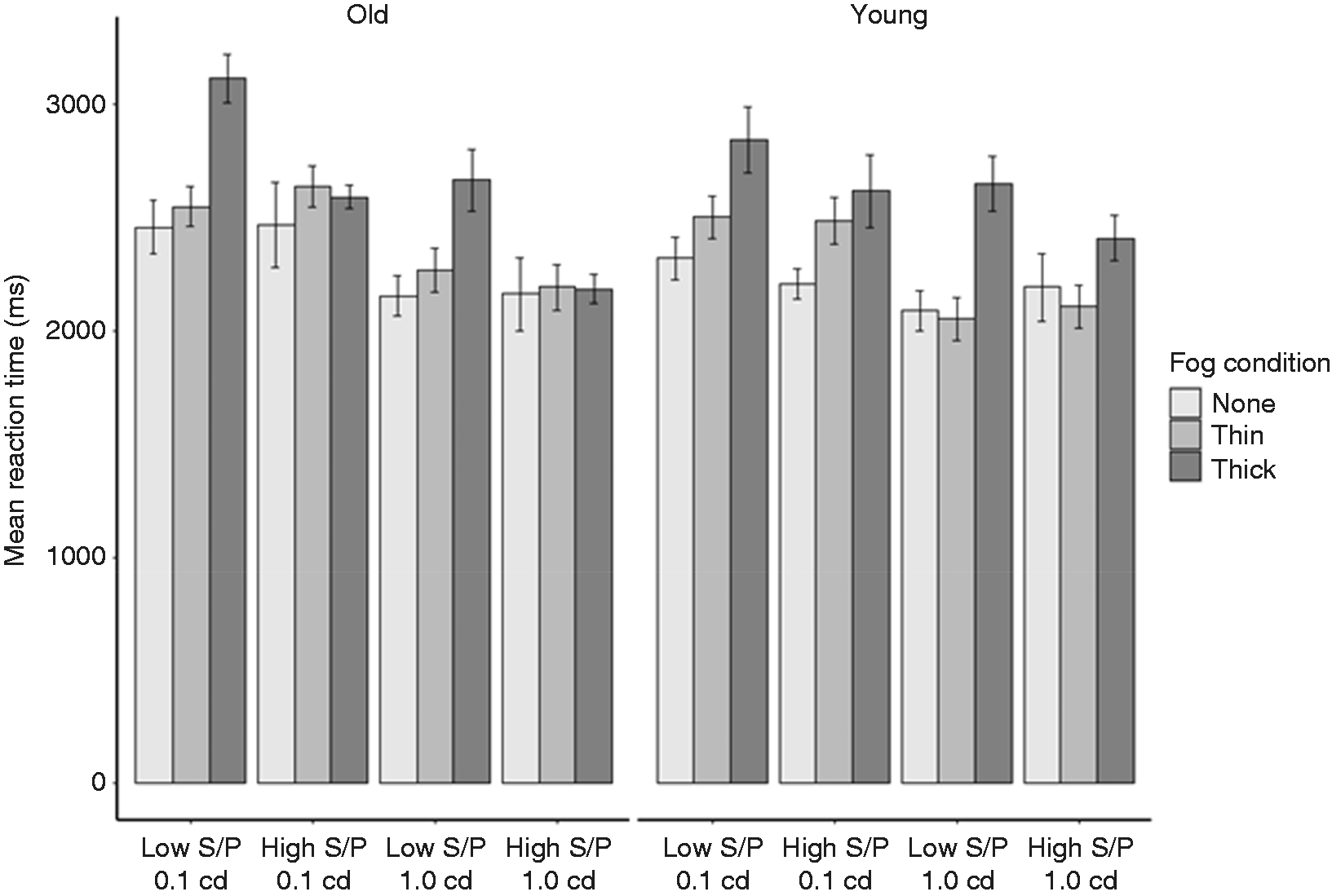

The linear mixed-effects model found significant main effects for luminance and fog condition. Reaction times were significantly shorter under 1.0 cd/m² luminance (mean = 2241 ms) compared with 0.1 cd/m² (mean = 2508 ms). Post hoc Tukey tests showed that the thick fog condition produced a significantly longer reaction time (mean = 2589 ms) than both no fog and thin fog conditions (means = 2247 ms and 2337 ms respectively, p < 0.005 in both cases). There was no difference between the no and thin fog conditions (p = 0.58). The only significant interaction was between S/P ratio and fog condition (F(2, 163) = 5.7, p = 0.004). This interaction is plotted in Figure 13, and suggests that whilst the S/P ratio of the lighting may not have influenced reaction times when there was no or thin fog, under thick fog conditions there was a difference, with faster reactions produced under the higher S/P ratio light compared with the lower S/P ratio light. Post hoc Tukey tests were unable to confirm this interpretation of the interaction effect, as the differences between spectra conditions for all three fog conditions were not found to be significant. However, repeated-measures t-tests comparing reaction times between the two S/P ratios for each of the three fog conditions found that whilst there was no significant difference for the no fog (low S/P mean = 2245 ms, high S/P mean = 2249 ms, p = 0.96) and thin fog (low S/P mean = 2329 ms, high S/P mean = 2344 ms, p = 0.70), there was a significant difference between spectra under thick fog conditions, with the high S/P ratio light producing shorter reaction times compared with the low S/P ratio light (low S/P mean = 2764 ms, high S/P mean = 2413 ms, p = 0.001).

Figure 13.

Mean reaction times for detection of obstacle by spectrum and fog condition. Error bars show the standard error of the mean.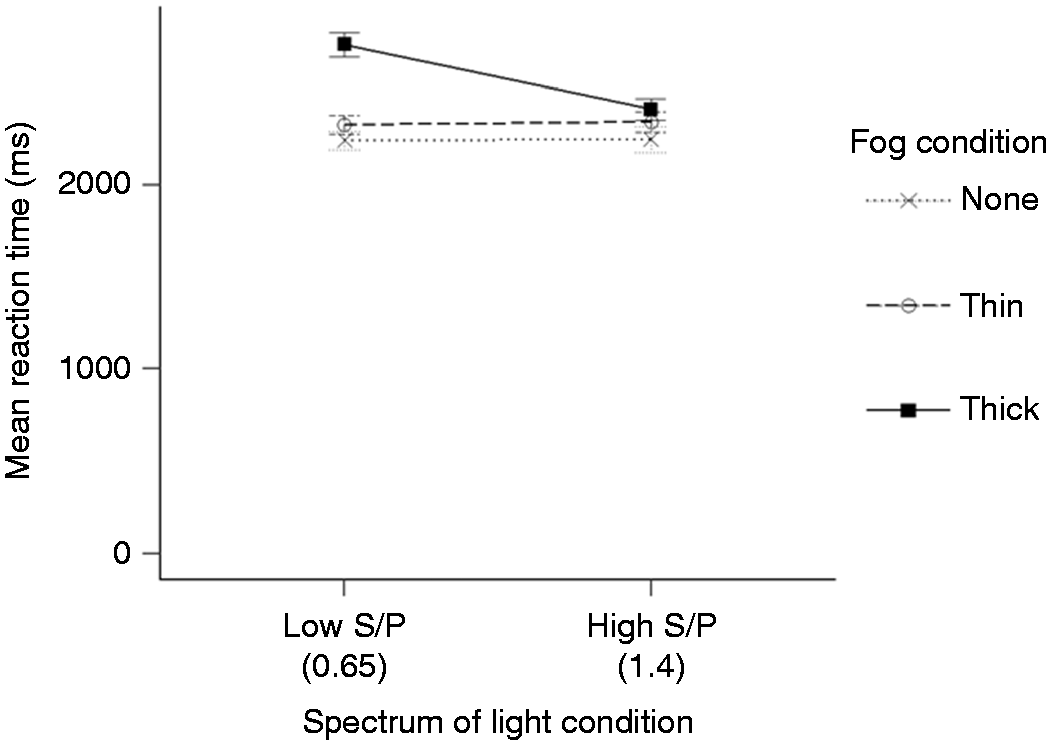

For consideration of collision avoidance note that reaction times were measured from first onset of movement of the obstacle. For the first second the obstacle was rising and hence subtended a smaller visual size, representing the approach to a more-distant obstacle, and a driver travelling at 70 mph would take approximately 1.5 seconds to reach the full-size obstacle at the simulated distance ahead of 47 m. This collision avoidance threshold of 2.5 seconds is the standard assumption for detecting and perceiving road hazards.³⁸

5. Discussion

The experiment tested the effect of light conditions on peripheral detection with two different luminances (0.1 cd/m² and 1.0 cd/m²) and two different SPDs (characterised by their S/P ratios, 0.65 and 1.4). Participants were generally better able to detect the car lane change and the obstacle under the higher luminance level, with detection rates being higher and reaction times being shorter for both the car and obstacle targets. An increase in luminance produced the greatest improvements under thick fog conditions. This suggests that a luminance of 1.0 cd/m² is particularly beneficial in foggy conditions compared with 0.1 cd/m². Although this may imply that a higher luminance will improve detection performance of drivers in thick fog, an important caveat to this is that we do not know what effect increasing the luminance beyond 1.0 cd/m² may have. It is possible that at higher luminances the amount of scattered light may begin to have a negative impact on visibility.³¹ Further research may be required to identify an appropriate luminance level for optimising visibility under conditions when fog density is greater than that used in the current trials. We also note that the target vehicles used for the lane change task did not use tail lights nor direction indicators which would otherwise contribute to detection of a lane change movement.

The difference in S/P ratios used in the experiment did not reveal any consistent effects on detection performance. The only possible effect related to S/P ratio was an interaction with the fog level and its effect on reaction times for detecting the obstacle. Under thick fog conditions, the light with the higher S/P ratio produced shorter reaction times. This is in line with expectations about the effects of S/P ratio – light with a higher S/P ratio is generally perceived as being brighter under mesopic conditions.³⁹ Previous work has also shown that shorter-wavelength light, typically with higher S/P ratios, produces higher perceived luminances than other types of light, particularly under fog conditions.⁴⁰

The experiment demonstrated that a higher luminance improved detection, particularly in thick fog conditions, and within the experiment’s parameters the higher luminance also equates to increased brightness. However, this effect of S/P ratio was not found for detection rates of the obstacle, or reaction times and detection rates for the car. No overall effect of S/P ratio on detection performance was found. One possible explanation for the minimal effects of spectrum measured in this experiment is that the detection tasks may not have been difficult enough. The effect of spectrum becomes magnified the closer a visual task is to the threshold levels of vision,⁵ and the more difficult a task is the closer it is to threshold levels. On this point, it is worth noting that an effect of S/P ratio was only revealed for the most difficult task (detection of the obstacle) and under the most reduced visibility conditions (thick fog). It is also worth noting that the lowest luminance used in this experiment was 0.1 cd/m². Previous work that has used similar detection tasks and experiment paradigms^28,33 only found an effect of spectrum at a luminance of approximately 0.01 cd/m², a log-unit difference from the lowest luminance used here. It is likely that an effect of the lighting S/P ratio may have been more evident at lower luminance levels.

These results suggest that thick fog reduces detection performance compared with no or thin fog. Reduced detection may lead to more collisions, and this can be seen in accident data. An analysis of 994 accidents occurring in Florida, 2003 to 2007, found that at speeds of 55 mph or higher (but not for lower speeds) the number of crashes was higher in fog than in clear conditions, and also that fog crashes were more likely to occur at night without street lighting.¹⁴ This suggests that street lighting can be beneficial as a counter measure to collisions in fog.

6. Conclusion

An experiment was carried out using a scale model to investigate how the detection of hazards in peripheral vision is affected by changes in light level (road surface luminances of 0.1 cd/m² and 1.0 cd/m²), S/P ratio (0.65 and 1.40) and fog density (none, thin and thick as defined by the absorption coefficient). Two types of hazards were used, a road surface obstacle and lane change of vehicles in adjacent lanes, and detection performance was measured using detection rate and reaction time. Increasing luminance, and reducing from thick to thin fog, led to significant increases in detection rate and reductions in reaction time, for both types of hazard. The effect of a change in S/P ratio was significant only when measuring detection of the surface obstacle using reaction times, under the thick fog, with an increase in S/P ratio leading to a shorter reaction time.

Footnotes

Declaration of Conflicting Interests

The authors declared no potential conflicts of interest with respect to the research, authorship, and/or publication of this article.

Funding

The authors disclosed receipt of the following financial support for the research, authorship, and/or publication of this article: This work was carried out in partnership with the Arup AECOM Consortium, funded by Highways England under TTEAR Work Package 584 – Impact of Road Lighting Review. The work was also supported by EPSRC Impact Acceleration Account EP/K503812.

References

Commission Internationale de l’Éclairage. Lighting of Roads for Motor and Pedestrian Traffic. CIE 115:2010. Vienna: CIE, 2010.

Olson

Sivak

. Comparison of headlamp visibility distance and stopping distance. Perceptual and Motor Skills 1983; 57: 1177–1178.

Plainis

Murray

Charman

. The role of retinal adaptation in night driving. Optometry and Vision Science 2005; 82: 682–688.

Plainis

Murray

. Reaction times as an index of visual conspicuity when driving at night. Ophthalmic and Physiological Optics 2002; 22: 409–415.

Bullough

Rea

. Simulated driving performance and peripheral detection at mesopic and low photopic light levels. Lighting Research and Technology 2000; 32: 194–198.

Rea

Bierman

Bullough

. Evaluating light source efficacy under mesopic conditions using reaction times. Journal of the Illuminating Engineering Society 1997; 26: 125–138.

Commission International de l’Éclairage. Recommended System For Visual Performance Based Mesopic Photometry. CIE 191:2010. Vienna: CIE, 2010.

Meteorological Office. What is Fog? Retrieved 19 December 2016, from http://www.metoffice.gov.uk/learning/fog.

Moore

Cooper

. Fog and Road Traffic. Transport and Road Research Laboratory Report LR 446. Crowthorne, UK: TRRL, 1972.

10.

Boyce

. Lighting for Driving, Boca Raton, FL: CRC Press, 2009.

11.

Rea

Ouellette

. Relative visual performance: a basis for application. Lighting Research and Technology 1991; 23: 135–144.

12.

Cavallo

Colomb

Doré

. Distance perception of vehicle rear lights in fog. Human Factors 2001; 43: 442–451.

13.

Brooks

Crisler

Klein

Goodenough

Beeco

Guirl

Tyler

Hilpert

Miller

Grygier

Burroughs

Martin

Ray

Palmer

Beck

. Speed choice and driving performance in simulated foggy conditions. Accident Analysis and Prevention 2011; 43: 698–705.

14.

Abdel-Atya

Ekram

A-A

Huang

Choi

. A study on crashes related to visibility obstruction due to fog and smoke. Accident Analysis and Prevention 2011; 43: 1730–1737.

15.

Hamilton

Tefft

Arnold

Grabowski

. Hidden Highways: Fog and Traffic Crashes on America’s Roads, Washington, DC: AAA Foundation for Traffic Safety, 2014.

16.

British Standards Institution, BS 5489-1: 2013 Code of Practice for the Design of Road Lighting. London: BSI, 2012.

17.

Alferdinck

. Target detection and driving behaviour measurements in a driving simulator at mesopic light levels. Ophthalmic and Physiological Optics 2006; 26: 264–280.

18.

British Standards Institution. EN13201-2:2015. Road Lighting. Part 2: Performance Requirements. London: BSI, 2015.

19.

Schoettle

Sivak

Flannagan

. High-beam and Low-beam Headlighting Patterns in the U.S. and Europe at the Turn of the Millennium, UMTRI-2001-19. Ann Arbor, MI: The University of Michigan Transportation Research Institute, 2001.

20.

Fotios

Cheal

Fox

Uttley

. The transition between lit and unlit sections of road and detection of driving hazards after dark. Lighting Research and Technology 2017. http://journals.sagepub.com/doi/full/10.1177/1477153517725775 .

21.

Walsh

Pearce

. The influence of automobile windscreen rake on effective light transmittance. Ophthalmic and Physiological Optics 2010; 30: 785–789.

22.

Bullough

Rea

. Impacts of fog characteristics, forward illumination, and warning beacon intensity distribution on roadway hazard visibility. The Scientific World Journal 2016. ; 8. Article ID: 4687816. DOI: 10.1155/2016/4687816.

23.

Olsen ECB, Lee SE, Wierwille WW. Analysis of distribution, frequency, and duration of naturalistic lane changes: Proceedings of the Human Factors and Ergonomics Society 46th Annual Meeting, 2002: pp.1789–1793.

24.

Green

. How long does it take to stop? Methodological analysis of driver perception-brake times. Transportation Human Factors 2000; 2: 195–216.

25.

Boyce

. Human Factors in Lighting,, 3rd Edition. Boca Raton, FL: CRC Press, 2014.

26.

Fotios

Uttley

Cheal

. Maintaining foveal fixation during a peripheral detection task. Lighting Research and Technology 2016; 48: 898–909.

27.

Winter

Fotios

Völker

. Gaze direction when driving after dark on main and residential roads: Where is the dominant location? Lighting Research and Technology. First published 17 February 2016. DOI: 10.1177/1477153516632867.

28.

Uttley

Fotios

Cheal

. Effect of illuminance and spectrum on peripheral obstacle detection by pedestrians. Lighting Research and Technology. 2017; 49: 211–227.

29.

Garland

. Some fog droplet size distributions obtained by an impaction method. Quarterly Journal of the Royal Meteorological Society 1971; 97: 483–494.

30.

Bohren CF. Atmospheric Optics. The Optics Encyclopedia. Wiley-VCH. Retrieved 15 September 2007, from http://onlinelibrary.wiley.com/doi/10.1002/9783527600441.oe004/abstract. DOI: 10.1002/9783527600441.oe004.

31.

Middleton

WEK

Vision through the atmosphere. In: Bartels

(ed). Geophysics II, Berlin: Springer-Verlag, 1957, pp. 254–287.

32.

Bierman

Raffucci

Boyce

DeCusatis

. Exit-sign degradation in smoke: a quantitative simulation. Lighting Research and Technology 1996; 28: 177–188.

33.

Fotios

Cheal

. Obstacle detection: a pilot study investigating the effects of lamp type, illuminance and age. Lighting Research and Technology 2009; 41: 321–342.

34.

Ikaunieks

le Colomb

Ozolinsh

. Light scattering in artificial fog and simulated with light scattering filter. Ophthalmic and Physiological Optics 2009; 29: 351–356.

35.

Otas

Pakenas

Vaskys

. Investigation of LED light attenuation in fog. Electronics and Electrical Engineering 2012; 5: 47–52.

36.

Tarel J-P, Hautière N, Cord A, Gruyer D, Halmaoui H. Improved visibility of road scene images under heterogeneous fog: Proceedings of the Intelligent Vehicles Symposium (IV), 2010; IEEE: pp. 478–485.

37.

Warrington

Tilling

Howe

Paternoster

Pennell

Briollais

. Robustness of the linear mixed effects model to error distribution assumptions and the consequences for genome-wide association studies. Statistical Applications in Genetics and Molecular Biology 2014; 13: 567–587.

38.

Rea

Bullough Zhou

. A method for assessing the visibility benefits of roadway lighting. Lighting Research and Technology 2010; 42: 215–241.

39.

Fotios

Cheal

. Predicting lamp spectrum effects at mesopic levels. Part 1: Spatial brightness. Lighting Research and Technology 2011; 43: 143–157.

40.

Kelly JMF, Smedley ARD, Carden D, Murray IJ, Webb AR. Explaining the high visibility of light emitting diodes in fog: Proceedings of the 28th CIE Session, 2015: pp. 1669–1775.

The effect of fog on detection of driving hazards after dark

Abstract

1. Introduction

2. Apparatus

2.1. Lighting

2.2. Detection tasks

2.3. Fog simulation

3. Procedure

4. Results and analysis

5. Discussion

6. Conclusion

Footnotes

Declaration of Conflicting Interests

Funding

References