The sunlight beam index

Abstract

This paper describes a fundamental rethinking of the basis for the evaluation of the sunlight potential of spaces. It provides a robust methodology to answer the question: how much sunlight can enter a room? The measure proposed is the cross-sectional area of beam sunlight that passes through a window. The new measure – called the sunlight beam index – is described, and examples are given for a realistic residential dwelling. The sunlight beam index is determined for a full year on a time-step basis (e.g. every 15 minutes), but it can be aggregated into monthly or yearly totals. The annual total provides a single measure for one window, a group of windows or all the windows for an entire dwelling.

1. Introduction

It is generally accepted worldwide that all dwellings should have occasional direct sun penetration through at least some of the windows. The same or similar criteria also apply to other categories of buildings, e.g. schools, residential/care homes, hospitals, etc. The guidelines for different countries/locales vary enormously though they tend to have similar key characteristics, e.g. that a window should receive direct sun for a certain period on, say, the equinox. For example, British Standard 8206-2 recommends that

“the centre of at least one window to a main living room can receive 25% of annual probable sunlight hours, including at least 5% of annual probable sunlight hours in the winter months between 21st September and 21st March. ¹ ”

A recent paper by Darula et al. lists the sunlight recommendations for 10 European countries. ² Three of them are reproduced in Table 1 to illustrate the range in the types of recommendations given.

Table 1

A selection of recommended sunlight duration requirements from Darula et al. ²

Country	Sunlight duration requirements
Czech Republic	At least 1.5 hours on March 1st or balance of sunlight duration in the period from February 10th to March 21st is at least 1.5 hours; solar altitude is at least 5°
Italy	At least 2 hours of sun per day in the period February 19th to October 21st
Sweden	At least one room or separable part of a room shall have access to direct sunlight; at least 5 hours sunlight between 9 am and 5 pm at spring and autumn equinox

This paper describes a new metric to assess the sunlight beam potential of arbitrarily complex building apertures, typically windows. The rationale for the new model is the need to create an index of sunlight beam potential for buildings that is a faithful measure of that actually experienced. As noted, existing measures of sun exposure/potential are many and various. However, they all possess one or more of the following weaknesses:

They consider only certain times of the day and/or year, e.g. one of the equinox conditions.

They either ignore the direction at which the sun is incident on the window, or employ crude switch mechanisms such as the ‘dead angle’.

They ignore the size of the window.

They ignore or cannot adequately account for the shadowing effects of frame bars or window reveals.

They ignore or cannot adequately account for shadowing caused by surrounding structures or buildings.

The method employed is restricted to idealised geometry or built forms.

The evaluation cannot produce a meaningful, aggregate measure for multiple windows and/or an entire dwelling.

The evaluation provides no information on the temporal dynamics of possible sun exposure.

The new model is an attempt to overcome all of the above deficiencies. Furthermore, the new model has all of the characteristics desirable for a robust methodology that could serve as the basis for guidelines and standards. A single, unambiguous measure of sunlight beam potential forms the basis of the new method. The evaluation considers all possible hours of the year when direct sunlight may illuminate a window. This paper describes the theoretical basis of the new metric and demonstrates its application to a realistic building model of a residential house.

2. Rationale for the new approach

The intention is to quantify the cross-sectional area of beam sunlight that enters an internal space through a glazed aperture, and to provide a meaningful measure of the cumulative annual potential of this occurrence. When sunlight passes through any aperture in a building (usually a window), the beam cross-sectional area can be reduced by four mechanisms:

If the angle of incidence θ is greater than zero, i.e. anything other than normal incidence.

The beam is blocked by any external wall/facade reveal depth (occurs whenever $\theta >0$ ).

The beam is blocked by any internal wall/facade reveal depth (occurs whenever $\theta >0$ ).

The presence of any additional external obstruction, e.g. balcony, neighbouring buildings, etc.

The first three of these mechanisms are illustrated in Figure 1. Assume that the beam and the glazed aperture have the same cross-sectional area: x². When the angle of incidence of the beam to the aperture normal is θ, the cross-sectional area of the beam passing through the aperture is $x^2\cos \theta$ in the absence of any internal/external reveal depths (i.e. for infinitely thin walls). In the presence of both external and internal reveal depths, the beam area is further reduced by the projecting structures (i.e. reveals) on the outside and inside of the window plane (Figure 1).

Figure 1

Mechanisms by which beam sunlight cross-sectional area entering a space can be reduced.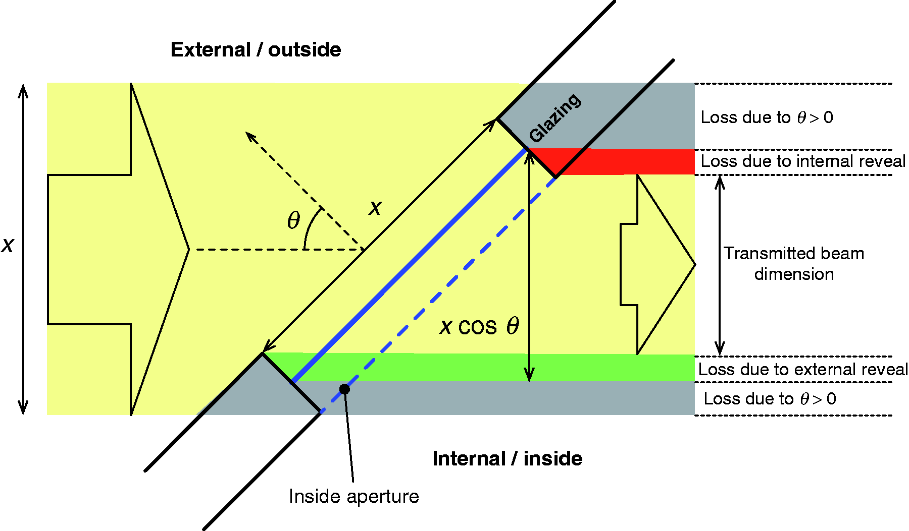

The preceding made reference to the window plane because this surface is invariably used in existing planning guidelines, etc., for the assessment of sunlight availability. Also, building refurbishment could result in an increase to either or both the external and internal reveal depths, e.g. due to added insulation. The position of the glazing plane, however, is usually unchanged when, say, insulation layers are added. The reduction in beam cross-sectional area due to the internal reveal depth is determined by calculating also the beam sunlight that enters the internal space through a ‘virtual’ inside aperture (Figure 1).

2.1. Theoretical basis

A single, unambiguous measure of sunlight beam potential forms the basis of the new method. Consider a glazed aperture of area A_g. When this area of glazing is illuminated by the sun at normal incidence for a period of time $\Delta t$ , the sunlight beam index (SBI) $S_{\Delta t}$ for that duration of time is equal to the product of the illuminated area A_i and the time period. Thus the SBI is a measure of the cross-sectional area and duration of direct sun beam that enters a space. ^a

a

Whilst SBI is analogous in nature to any flux-related quantity, there is no actual measure of ‘flow’ since the beam of sunlight for this purpose is treated as an instantaneous entity.

For the case of normal incidence with no obstructions (i.e. A_i = A_g):

$S_{\Delta t}=A_g\Delta t$

(1)

However, when the angle of incidence θ is greater than 0°, the SBI is reduced by the cosine of the angle because the cross-sectional area of the transmitted beam is reduced by that amount. Thus, the illuminance at the window plane serves as a proxy for the reduced cross-sectional area of the transmitted beam:

$S_{\Delta t}=A_g\cos \theta \Delta t$

(2)

Most window glass will be fixed in a frame that stands proud ‘above’ the surface of the glass, i.e. the glass is, in effect, recessed within the frame. Thus, any direct sun illumination on the glass at non-normal incidence will result in the frame and/or reveal casting a shadow onto the glass. In other words, the illuminated area of glass will be less than the total area of the glazed aperture, i.e. A_i < A_g. The area of glass in shade (or ‘umbra’) is A_u:

$A_g=A_i+A_u$

(3)

Shading of direct sun can also result from any other structure, nearby (e.g. balcony) or more distant (e.g. obstructing tall building). The angle and obstruction effects are illustrated in Figure 2. Combining the angle and obstruction effects, the generalised SBI equation is:

$S_{\Delta t}=A_i\cos \theta \Delta t=(A_g-A_u)\cos \theta \Delta t$

(4)

With the area given in square metres and the time period given in hours (or more typically, a fraction of an hour), the SBI has units of square meter per hour. This formulation makes good sense for a number reasons:

• It is consistent with fundamental illumination physics (e.g. the cosine law of illuminance as a proxy for reduced area of cross-sectional beam).

• The penetration depth of the sun’s rays into the space will be reduced with increasing angle of incidence.

• Large incidence angle sun illumination on the window will have a proportionate (i.e. small) contribution in any evaluation without requiring any recourse for arbitrary cut-off conditions, e.g. ‘dead angles’, etc.

• The glazed area is properly accounted for.

• Shading – whatever its origin – is properly accounted for.

Any meaningful evaluation must account for the entire year of possible sun positions to capture all of the potential occurrences of sun and, importantly, shading also. How this is done is described in the following section.

Figure 2

Angle and shading effects in the evaluation of the sunlight beam index.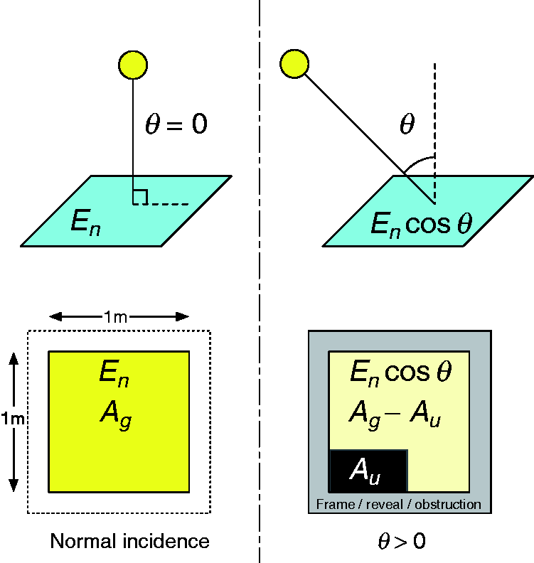

2.2. Annual SBI

The total SBI S_tot for any glazed aperture – or group of glazed apertures – is the sum of all the individual sunlight beam indices for the entire year where the sun altitude γ_s is greater than zero:

$S_{\mathrm{tot}}=\sum _{{\gamma }_s>0}(A_i\cos \theta \Delta t)$

(5)

Additionally, the individual values of $S_{\Delta t}$ for the entire year can be used to populate a 2D matrix that can be visualised as a temporal map (TM) T, which has dimensions 24 × 365 for hourly data (i.e. $\Delta t=1$ hour):

$\mathbf{T}=[S_{1,1}{S}_{1,2}\dots \mathrm{\hspace{1em}\hspace{1em}\hspace{1em}}{S}_{1,365}{S}_{2,1}{S}_{2,2}\dots \mathrm{\hspace{1em}\hspace{1em}\hspace{1em}}{S}_{2,365}::S_{24,1}{S}_{24,2}\dots \mathrm{\hspace{1em}\hspace{1em}\hspace{1em}}{S}_{24,365}]$

(6)

For a time-step of 15 minutes, the TM array has dimensions 96 × 365. For a space with n multi-aspect windows (or window groups) labelled a, b, etc., the total SBI for the space is simply the sum of the individual SBIs:

$S_{\mathrm{space}}=S_a+S_b+\dots +S_n$

(7)

Similarly, the TM for the space is the sum of the individual TM arrays:

${\mathbf{T}}_{\mathrm{space}}={\mathbf{T}}_a+{\mathbf{T}}_b+\dots +{\mathbf{T}}_n$

(8)

If required, the total SBI for a dwelling or building can be obtained by summing all SBIs for the relevant windows or window groups. Thus, it becomes possible to characterise the SBI for an entire building (e.g. dwelling) with is single SBI value.

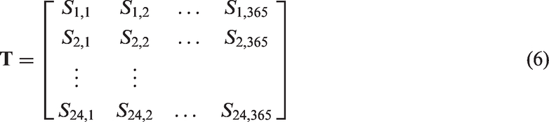
The combining of individual TM arrays allows for the creation of a visual algebra, whereby the temporal dynamics of sunlight beam for an entire building of arbitrary complexity can be readily conveyed to, say, the designer. For example, the TMs for individual windows can be incrementally summed (or subtracted) to immediately reveal – and communicate – the effect of design changes/options.

2.3. Computation of SBI

The Radiance lighting simulation system was used as the ‘engine’ in the implementation described here. ³ In fact, the SBI simulation tool used was a subset of a generalised climate-based daylight modelling (CBDM) tool referred to as the ‘4 component’ method. ⁴ Note, however, that lighting simulation per se is not required to compute SBI because the method depends only on a line-of-sight calculation; the modelling of inter-reflection and/or the transmission/scattering effects of light are not needed. Thus, SBI could in principle be computed by any 3D CAD/BIM tool that can determine whether there is line-of-site visibility between two points: one in the building model, the other at a sun position on the sky vault.

The accuracy and precision of the computed SBI depends primarily on the faithfulness of the 3D model. In short, good geometry should ensure a reliable result. Simulation parameters which have an influence on the outcome are:

the simulation time-step combined with the sun discretisation scheme (these two are related), and

the density of the sensor grid at the window aperture.

The setting of these parameters is essentially arbitrary, incurring only an overhead in computational resources. For the examples shown in this paper, a 15-minute time-step was used, i.e. the sun position was determined at 15-minute intervals for an entire year. Potential sun positions on the sky vault at each time step were taken from a pre-determined set of 2056 evenly distributed points. In the ‘4 component’ CBDM tool, these points are used to compute the daylight coefficient matrix for the direct sun component of illumination. ⁴ The divergence between an actually occurring sun position (at each time step) and the nearest pre-computed point on the sky vault was never greater than 2.3°. This granularity in spatial discretisation for the pre-computed sun positions is comparable with a time-step of approximately 9 minutes, i.e. approximately commensurate with the 15-minute time-step used for the computation of SBI. There would be no advantage with regards to the accuracy of the predicted SBI if there were a significant mismatch between these two time-step values.

The density of the sensor grid at the window aperture was determined by indirect means using an approach, which is commonly known as the ‘stencil method’. The ‘stencil method’ is described in Appendix 1 together with an illustration demonstrating the scalability of the Radiance-based tool to compute SBI.

3. SBI illustration

3.1. One metre square aperture

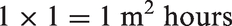
Consider a 1 m by 1 m square glazed aperture. When this is illuminated at normal incidence by the sun for a period of 1 hour, the SBI for that period is:

$1\times 1=1{\text{m}}^2\text{hours}$

In other words, a beam of sunlight with a cross-sectional area of 1 m² passed through the window aperture for a period of 1 hour. If instead, the glass were illuminated at an angle of incidence of 60° for the same 1-hour period, the SBI would be:

$1\times \cos 60\times 1=0.5{\text{m}}^2\text{hours}$

because, at 60° incidence, the cross-sectional area of the transmitted beam is half what it was at normal incidence. Additionally, the glazed area may be partially shaded by the window reveal and/or external structures. Say, 0.3 m² of the glazed are is in shade, giving an illuminated area 0.7 m². The SBI would now be:

$0.7\times \cos 60\times 1=0.35{\text{m}}^2\text{hours}$

3.2. Annual SBI

The annual sunlight beam on the 1 m² window aperture in the vertical plane was predicted using clear sunny skies for a full year. The geographical locale used to generate the sun positions was London (UK), and a time-step of 15 minutes was used, i.e. there were approximately 17,520 above horizon sun positions accounted for in the evaluation. The SBI was simulated for the window in eight orientations: the cardinal and mid-cardinal compass points. This was done for both an unobstructed window aperture and one set in a 20 cm reveal depth. The results are shown in Table 2. Immediately evident is the expected large variation in SBI with respect to orientation. The aperture reveal depth also has a significant effect, and across all orientations. For example, for the south facing orientation, it reduces the SBI from 1927 to 1340 m² hours.

Table 2

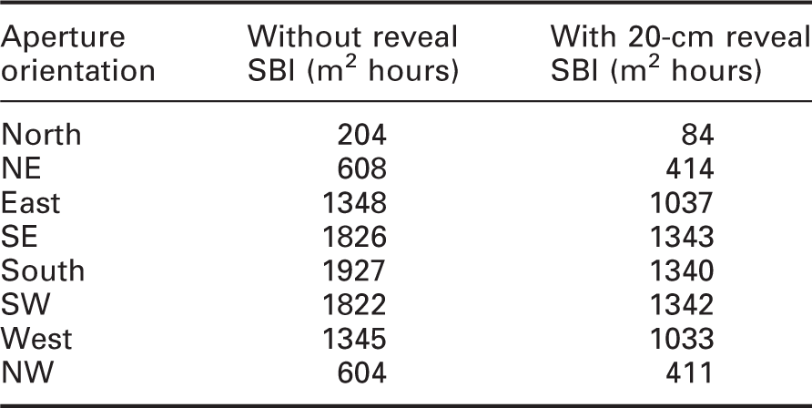
SBI for 1 m² glazed aperture without and with 20-cm external reveal depth

Aperture orientation	Without reveal SBI (m2 hours)	With 20-cm reveal SBI (m2 hours)
North	204	84
NE	608	414
East	1348	1037
SE	1826	1343
South	1927	1340
SW	1822	1342
West	1345	1033
NW	604	411

3.3. TM example: One window

An example sunlight beam TM is given in Figure 3. This example is for window (glaz01) on the upper story of a residential building. For this building orientation (135° clockwise rotation from north), the window faces south-east, i.e. also 135°. The building location for this example is Ostersund, Sweden. From the TM, the pattern of night (dark grey) and day (light grey or colour) is clearly visible. Daytime light grey indicates that the sun is above the horizon but has no direct visibility of any part of the window area either because the sun is ‘behind’ the window (i.e. angle of incidence > 90°) or it is blocked by local obstructions. Where there is an evident light grey ‘notch’ in the pattern of colour, this usually indicates that the window is being shaded by some local obstruction (surrounding buildings were present in the model). A yellow shade indicates that sun can be incident on the window at near normal incidence. Whereas a blue shade indicates large angle of incidence direct sun and/or significant obstruction.

Figure 3

Temporal map example. (Available in colour in online version)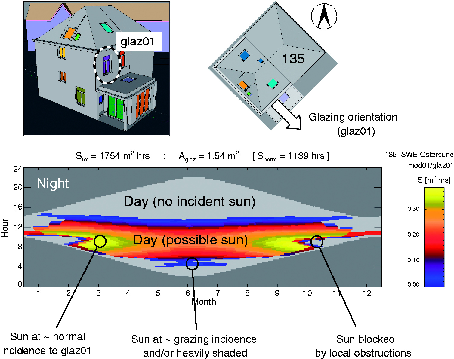

The plot title contains the following: The annual total SBI (1754 m² hours), the area of the glazed aperture (1.54 m²), and the normalised annual total SBI (1139 hours). The normalised annual total SBI is simply the annual total SBI divided by the area of the glazed aperture. The normalised annual total can be taken to be a SBI ‘efficiency’ measure, which could be used to make comparison between various window types and/or arrangements.

3.4. TM example: Complete dwelling

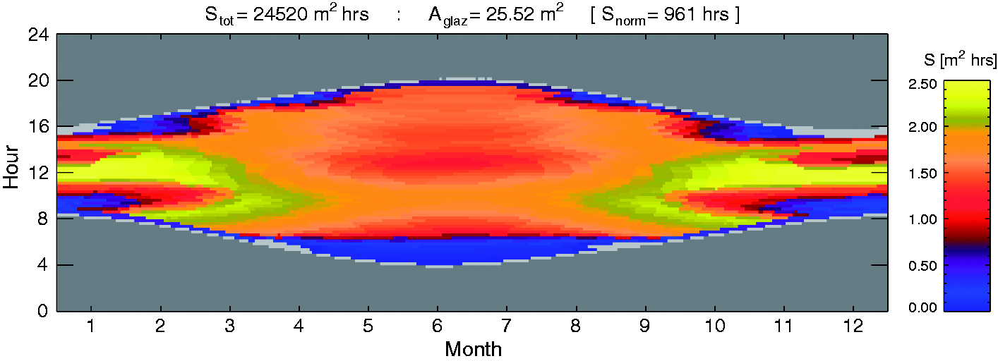
For this illustration, TMs were generated for all 16 windows of the house used in the previous example. There are 16 glazing groups for 10 distinct space types, Figure 4. This ‘Row House’ model is surrounded by neighbouring houses (not shown), and the effect of horizon obstructed by houses in the distance is accounted for by an ‘enclosing’ cylinder. The combined TM for the entire dwelling is shown in Figure 5. The numerical total for SBI across the year was 24,520 m² hours – a single figure can characterise the sunlight beam potential of an entire dwelling.

Figure 4

Glazing elements/groups in the ‘Row House’ model.

Figure 5

Summed temporal map for the entire dwelling (all 16 window groups). (Available in colour in online version)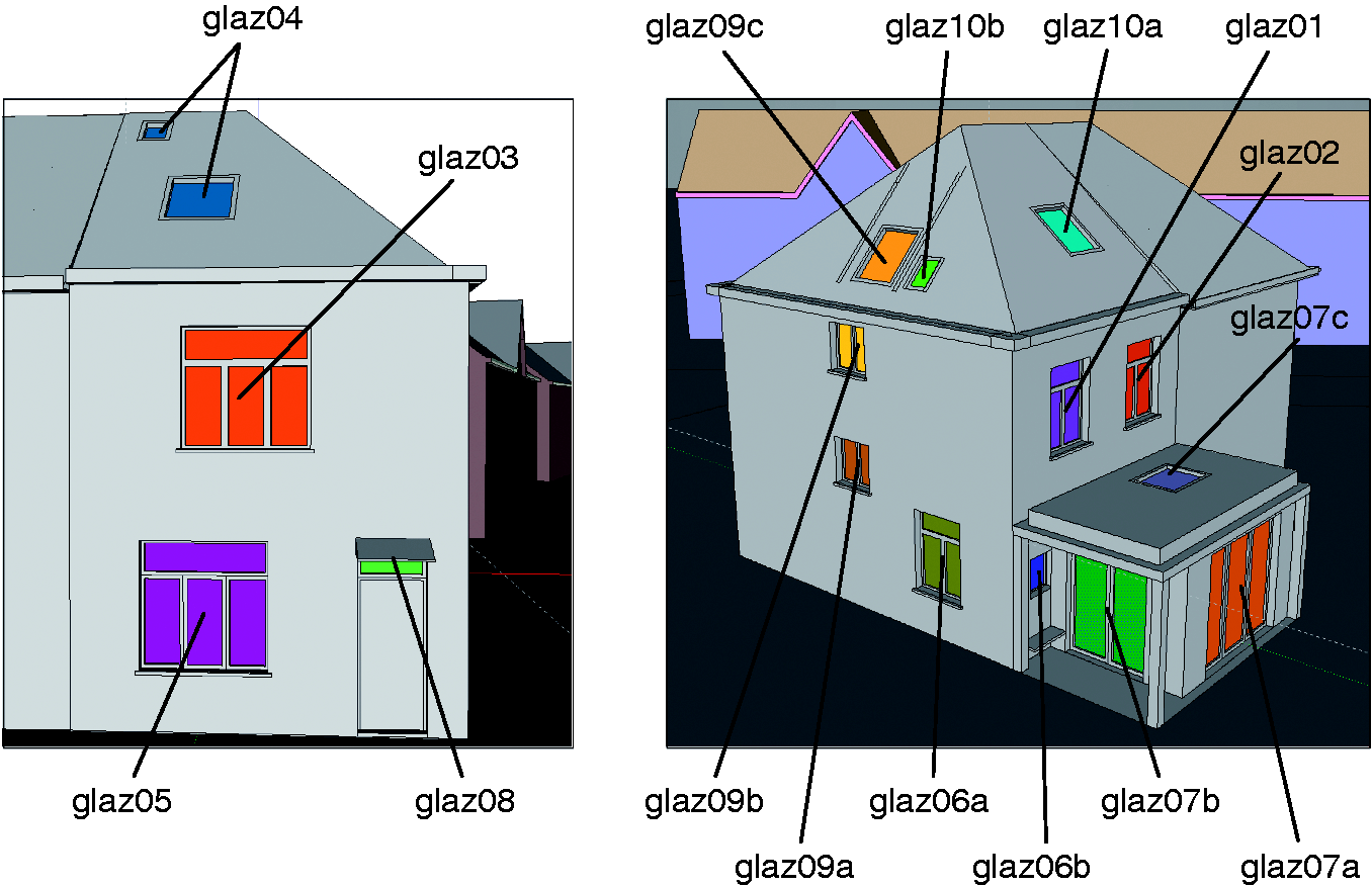

Eight of the 16 TMs are shown in Figure 6. This figure is best viewed on-screen and enlarged. Note that the false colour scale varies according to glazing area for each window or window group. At a glance, one can appreciate the patterns in annual sunlight beam potential for the entire house on a window group by window group basis. This visual presentation of data becomes particularly effective when comparing, say, the TMs for the same house design given different orientations. Quite dramatic difference in the patterns of annual SBI are observed for changes in orientation, and the approach would appear well-suited for the evaluation of housing masterplans, etc.

Figure 6

Eight of the 16 SBI temporal maps for the Row House model. (Available in colour in online version)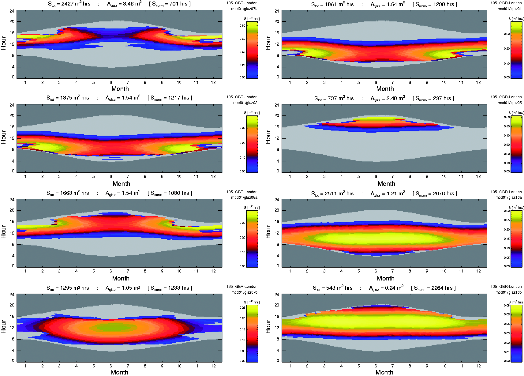

3.5. Effect of internal reveals on SBI

As noted in Section 2, any non-zero internal reveal depth will lead to a reduction in the cross-sectional area of any beam that passes through the window aperture (for all $\theta >0$ ). The beam sunlight that enters the main volume of the space (i.e. that is not ‘lost’ in the internal reveal) is determined in the same manner as above, only now an ‘inside aperture’ parallel to the window serves as the calculation grid. The internal aperture is flush with the internal wall boundary and entirely covers the window opening (from this position). In other words, any beam sunlight that passes through the window aperture must pass through the internal aperture to enter the space, Figure 7 (see also Figure 1). The internal aperture is often larger that the window due to the presence of the frame. Note that, any window frame in front of the glazing aperture can block beam sunlight in the same way as the external reveal. Similarly, any window frame ‘behind’ (i.e. inside) the glazing aperture can block beam sunlight the same as the internal reveal.

Figure 7

Model showing internal (250 mm) and external (50 mm) reveal depths for 300-mm wall.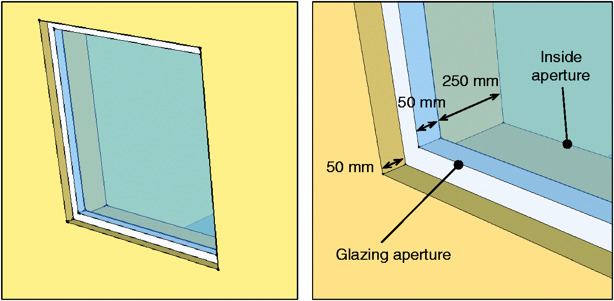

The effect of internal reveal is demonstrated for two wall thicknesses: 300 and 600 mm (the latter indicating a very thick, super-insulated wall). In each case, the external glazing surface has a 50 mm recess (or external reveal), resulting in internal reveal depths of 250 and 550 mm. The glazing area for the model shown in Figure 7 was 1.21 m² (same for the model with the thicker wall). The glazing orientation was due south and the SBI predicted for a London (UK) location. The results are summarised in Figure 8. The bar chart shows the monthly SBI totals for three internal reveal depths: 000 mm (i.e. same as that calculated at the glazing aperture), 250 mm, and 550 mm. The plot is annotated with the annual total for each case. Also shown are the three corresponding TMs. From the annual totals, approximately a quarter of the beam sunlight that passes through the window is ‘lost’ in the 250-mm deep window reveal, and more than half in the 550-mm deep reveals. As expected, the blocking effect of the internal reveal is greatest in the summer months when the angle of incidence between the sun and the window normal is greatest.

Figure 8

Effect on internal reveal depth on sunlight beam index. (Available in colour in online version)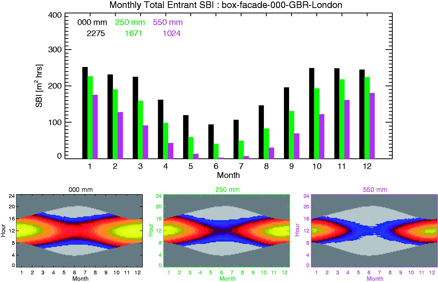

3.6. Volumetric assessment of beam sunlight

For this final part of the exposition of this new approach, the potential to make some meaningful aggregate measure and visualisation of the volume of space ‘penetrated’ by direct beam sunlight is investigated. For this, a very simple space is used: height × width × depth was 3 m × 3 m × 5 m, with a 1 m × 1 m glazed aperture positioned centrally in one of the walls, Figure 9(a). The sensor array is now a ‘stack’ of 12 sensor grids separated by 10-cm intervals, and starting from a height of 5 cm above the floor. Thus, the sensor array accounts for a volume of height 1.2 m above the floor. This was chosen because this is typically the ‘occupied’ height above the floor for people seated in a space. To be consistent with daylight simulation recommendations, there is a 0.5-m perimeter space between the sensor array and the walls, i.e. each sensor plane has dimensions 2 m × 4 m. ⁵ Each point on the sensor arrays now represents a volume element (or voxel) rather than an area.

Figure 9

Volumetric display of sunlight beam potential. (Available in colour in online version)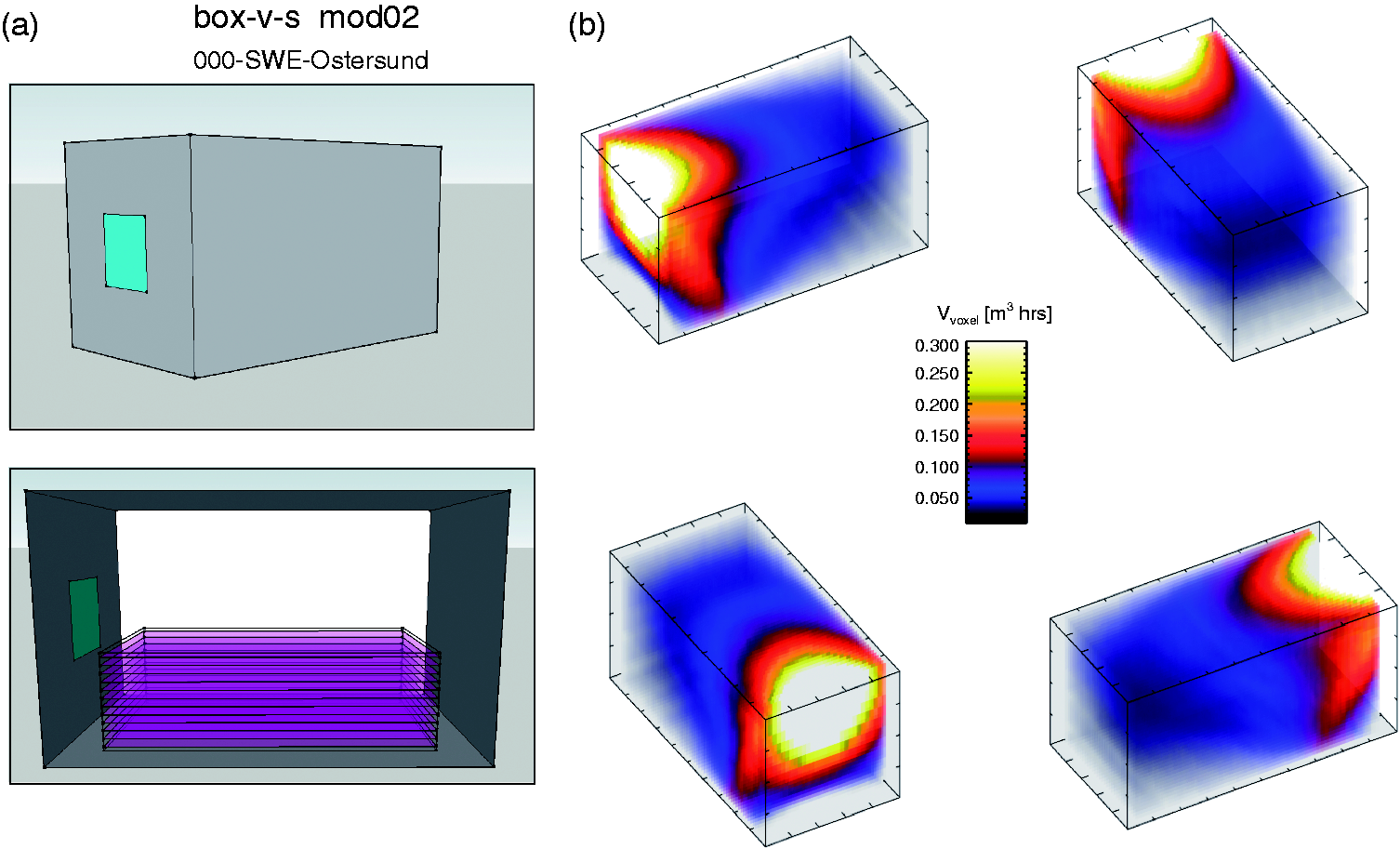

The simulation was run as before for a full year at a time-step of 15 minutes and, for this illustration, the location of the room was Ostersund (Sweden) and the window aperture was facing due south. For each time-step $\Delta t$ that sunlight was incident on a sensor array point (voxel volume v m³), the volumetric sunlight beam potential at that point is simply $v\Delta t$ m³ hours. The annual total is then the sum of the individual voxel values over the year.

A volumetric rendering of the total annual sunlight beam potential is given in Figure 9(b) – four views of the same volume are given. For this rendering of 3D data, the voxel opacity is proportional to the magnitude of the value at that point. Thus, the very low values (shaded black) are given a very low opacity and so appear as a ‘grey haze’ allowing the viewer to ‘see through’ to the shaded higher values (yellow/white). Additionally, it is also possible to determine a single numerical total volumetric potential for beam sunlight – for this case, it was 1785 m³ hours. It remains to be determined how best to interpret and apply measures of the volumetric potential of beam sunlight in spaces.

4. Discussion

This paper has described what is, in effect, a fundamental rethinking of the basis for the assessment and quantification of sunlight potential in spaces. The approach is founded on the long-term quantification of the cross-sectional area of beam sunlight that can enter a space. The approach accounts for all potential losses due to obstructions of any kind and at any scale. Furthermore, the approach distinguishes between losses calculated at the window plane, and those due to the internal construction of the building (e.g. internal sill depth). The graphical/numerical outputs have varying degrees of granularity: the SBI can be presented as a TM for one or more windows (i.e. every value for the year at, say, a 15-minute time-step), or aggregated into monthly/annual numerical totals. The approach is highly scalable and can accommodate any practical building geometry constructed using a CAD/BIM system.

The inherent simplicity and scalability of the approach described in this paper indicates that it could form a common basis for the evaluation of sunlight across, say, the EU/CEN countries. Although the existing guidelines vary considerably from one country to the next, the purpose of each is to make some meaningful assessment of sunlight potential. ² The work described here will be expanded upon to determine its applicability as a basis for future EU/CEN guidelines. This will involve an evaluation of SBI alongside a variety of the measures recommended in current European guidelines/legislation.

No mention has been made thus far regarding glazing transmissivity and its effects on SBI. This is another area to be explored as it would require the evaluation of absolute values for the intensity of the transmitted sunlight beam. This in turn leads to a consideration of the prevailing climate as an indicator of the likely occurrence of sunny conditions throughout the year. To account for the attenuation of SBI due to glazing transmission – including its angular dependency – the sensor grid is placed just ‘behind’ (instead of just in ‘front’ of) the glazing. The window is now modelled with the correct transmission properties for the particular glass type. A maintenance factor accounting for reduced transmissivity due to dirt could also be included. In 2003, the World Meteorological Organization (WMO) defined sunshine duration as that period during which the direct solar irradiance exceeds 120 Wm⁻². ⁶ Applying local climate data, and using the WMO definition as a threshold, the SBI approach could readily be extended to determine the prevailing intensity of entrant sunlight beam as well as its cross-sectional area over time. It remains to be determined how best such measures could be used to quantify entrant sunlight as it is experienced by building occupants.