
Abstract
In management research, fixed alpha levels in statistical testing are ubiquitous. However, in highly powered studies, they can lead to Lindley’s paradox, a situation where the null hypothesis is rejected despite evidence in the test actually supporting it. We propose a sample-size-dependent alpha level that combines the benefits of both frequentist and Bayesian statistics, enabling strict hypothesis testing with known error rates while also quantifying the evidence for a hypothesis. We offer actionable guidelines of how to implement the sample-size-dependent alpha in practice and provide an R-package and web app to implement our method for regression models. By using this approach, researchers can avoid mindless defaults and instead justify alpha as a function of sample size, thus improving the reliability of statistical analysis in management research.
Keywords
The rule of thumb quite popular now, that is, setting the significance level arbitrarily to .05, is shown to be deficient in the sense that from every reasonable viewpoint the significance level should be a decreasing function of sample size. Leamer (1978: 92)
Statistical analysis is often used to estimate the effect of one variable on another. Or, more precisely, to give a range of estimates that accounts for uncertainty: a confidence interval. While this interval is useful, researchers typically wish to also state whether an effect exists. Do acquisitions cause employees to leave? Do successions from a non-family CEO back to a family CEO reduce labor costs? Do university entrepreneurship programs promote entrepreneurship? These questions—or hypotheses—require a binary answer: yes or no. To answer such questions empirically, researchers often rely on null hypothesis significance testing (NHST). NHST is a statistical procedure that can govern researchers’ behavior toward whether a hypothesis is true while ensuring that they are not wrong too often (Neyman et al., 1933). To reach such a conclusion, a significance threshold at which to reject a hypothesis must be chosen.
Every part of the research process should be justified (Aguinis et al., 2018, 2021) yet discussions regarding the significance threshold—the alpha level—have been almost entirely absent from the management literature (for an exception, see Aguinis et al., 2010). This choice should be justified before data collection and should not be based on the idea of “one alpha to rule them all” (Lakens et al., 2018a: 169). Yet, justification for the alpha level is exceedingly rare in management research; arbitrary thresholds such as 0.10, 0.05, 0.01, and 0.001 abound (Aguinis and Harden, 2009). These thresholds act as gatekeepers for whether a result is deemed valuable or not (Bettis et al., 2016). From 2002 to 2006, 99% of papers in top management journals relied on these conventional values for α, making management the business discipline that has most strongly embraced this tradition (Aguinis et al., 2010). It is fair to say that “[p]articular p-values (0.05, 0.01, or 0.001) have been endowed with almost mythical properties” (Bettis et al., 2016: 259).
Unfortunately, relying on a universal α, such as 0.05, is problematic. With a large sample, p-values lower than conventional alpha levels can be more likely under the null hypothesis than the alternative. This phenomenon—known as Lindley’s paradox (Wagenmakers and Ly, 2021)—occurs because the distribution of p-values is a function of the sample size (Cumming, 2008). Management researchers who subscribe to Bayesian statistical philosophy have already identified this as a major limitation of NHST (Certo et al., 2022): with a fixed alpha, “[s]tatistical significance is an easy goal because any researcher can achieve it by adding more data” (Starbuck, 2016: 61) or, put differently, “[a] researcher who gathers a large enough sample can reject any point-null hypothesis” (Schwab et al., 2011: 8). With the era of big data creeping ever more into management research (Barnes et al., 2018; Wright, 2016), this problem becomes more serious; it is now standard to work with thousands, if not tens of thousands, of observations. 1
In this article, we propose a principled and practical way of lowering the alpha level as the sample size increases. This approach ensures the null is only ever rejected when it is less likely than the alternative. Researchers can thus enjoy the long-run Type I error rate guarantees of NHST while interpreting a significant test as evidence for the alternative hypothesis in a Bayesian fashion. Our solution to Lindley’s Paradox can be seen as a frequentist/Bayesian compromise. Indeed, it brings Bayesian and frequentist statistics closer together by solving the large-n conflict that arises when a fixed alpha is used.
Our solution extends the work of Maier and Lakens (2022), who recently proposed a Bayesian/frequentist compromise for justifying the alpha level in psychology research. Maier and Lakens (2022) build a bridge between p-values and Bayes factors for analysis of variance (ANOVA) and simple t-tests. In this article, we extend their method to allow for all standard generalized linear regression models, including linear, logistic, and Poisson regression, among others. We achieve this by relying on recent advances in the methodological development of Bayes factors (Mulder et al., 2021), specifically the approximate adjusted fractional Bayes factor (Gu et al., 2018). To ease use, we provide a practical workflow in Table 1, an R-package, and a Shiny web app.
Summary of recommendations for setting alpha based on sample size.
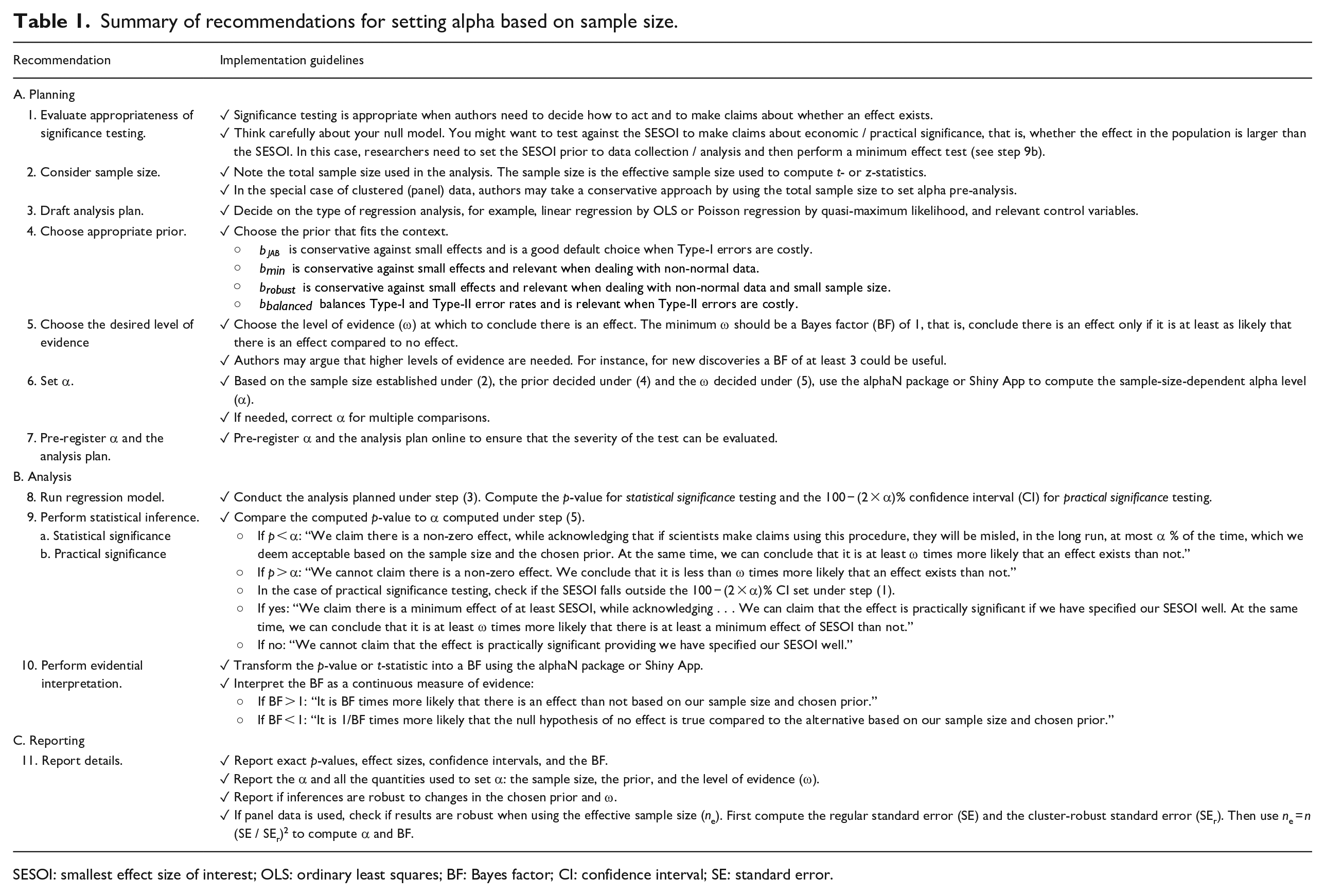
SESOI: smallest effect size of interest; OLS: ordinary least squares; BF: Bayes factor; CI: confidence interval; SE: standard error.
The issues of NHST have long been acknowledged. Indeed, in the last decade, many prominent journals have removed all significance thresholds from their publications. While choosing no threshold necessarily means choosing no arbitrary threshold, we argue that this does not solve the problem. Those who consume research (fellow researchers, industry professionals, and policymakers) do so to inform decisions. Whether academic articles include thresholds or not, readers still require a decision threshold: should I take action based on this result? Thus, such journal policies do not negate the need for our method. We encourage readers of any study to use our approach irrespective of the alpha level used (or lack thereof) by the authors of the study. Thus, even if researchers themselves are no longer responsible for choosing sensible thresholds, those who use research, and those who judge the usefulness of research (journal editors and referees), still require guidance. Indeed, our approach can act as a guidepost for editors and referees to point researchers to, such that their journal maintains consistency in their NHST protocols.
We hope that besides consumers and judges of research, researchers themselves can use our guidance to inform good research practice when carrying out NHST, interpreting results, and reporting statistical significance (see Table 1 for details, Appendix 3 for a checklist, and Appendix 4 for a suggested reporting format). We also emphasize that our approach can—and should—be used in conjunction with tools designed to investigate practical significance, such as confidence intervals and smallest effect size of interest (SESOI) testing.
We do not wish our message to be seen as a negative one. Using our approach, it will be more difficult to find statistical significance when using large samples. But if a large sample is required to uncover such effects, it is likely they are of little practical importance. Furthermore, an alpha that shrinks as the sample size increases, is one that grows as the sample size decreases. For research that relies on small samples, our method provides good reasons to increase alpha; with a sample size of 150, an alpha of 11% can be well justified using our method.
The rest of this article is organized as follows. First, we recap the basics of NHST and the issues with fixed alpha levels. We then discuss existing solutions and why they are deemed inappropriate, before giving our solution. Finally, we discuss practical implementation using previous papers as examples. Table 1 contains a full guide for use. For immediate implementation, the Shiny app can be accessed at https://crossvalidated.shinyapps.io/alphaN/, or the R package alphaN can be used.
Significance testing and alpha levels
NHST is widely considered the dominant approach for statistical inference in quantitative management research (Lockett et al., 2014; Van Witteloostuijn, 2020). NHST is appropriate when researchers must decide how to act with respect to a given hypothesis. If a researcher would like to know whether they can make a scientific claim about an effect, they set up a null hypothesis. For instance, if a researcher is interested in knowing whether inter-divisional knowledge sharing in an organization leads to more inventions, they can set up the null hypothesis

where T is the test statistic that quantifies the incompatibility with
This procedure, known as the Neyman–Pearson approach to statistical inference, allows researchers to make binary claims while controlling the error rate (Lakens, 2021). If a researcher rejects
Here, a researcher wishes to make a claim about a population, yet they only have access to a sample. In NHST, a researcher can be wrong in two ways: rejecting a true
Problems with a fixed alpha level
Conventional α levels can be traced back to Ronald A. Fisher, one of the fathers of frequentist hypothesis testing, who often used an α of 0.05 or 0.01. However, neither Fisher, Neyman, nor Pearson recommended a universal threshold (Maier and Lakens, 2022). For instance, Fisher (1971) explains that “[i]t is open to the experimenter to be more or less exacting in respect of the smallness of the probability he would require before he would be willing to admit that his observations have demonstrated a positive result.” Similarly, Neyman et al. (1933) made it clear that
[f]rom the point of view of mathematical theory all that we can do is to show how the risk of the errors may be controlled and minimized. The use of these statistical tools in any given case, in determining just how the balance should be struck, must be left to the investigator.
A Neyman–Pearson perspective
From a Neyman–Pearson perspective, it is logical that α should be a decreasing function of the sample size. As previously explained, Type I and Type II errors can occur when performing NHST. For a single study, the combined probability of a Type I or Type II error, ω, is the mean of α and β (Mudge et al., 2012).
The upper left of Figure 1 illustrates the relationship between α and the average error (ω) for a two-sample, two-sided t-test with a true effect size of 0.5 (equivalent to a regression on a single binary variable). In general, the average error rate falls as the α level decreases. However, below a certain point, the relationship reverses and the average error rate increases as α decreases. Furthermore, this change occurs at smaller α levels when the sample size is larger. Thus, for different sample sizes, we can identify the combination of α and β that minimizes the combined probability of Type I and Type II errors (Mudge et al., 2012). The upper right of Figure 1 shows how the α that minimizes the average error is a decreasing function of the sample size. For a sample size of 100, the optimal α is 0.0506, close to the conventional threshold of 0.05. At n = 200 the optimal α is 0.0085 and thus lower than conventional thresholds. Clearly, fixing α for different sample sizes is not optimal for overall error rates.
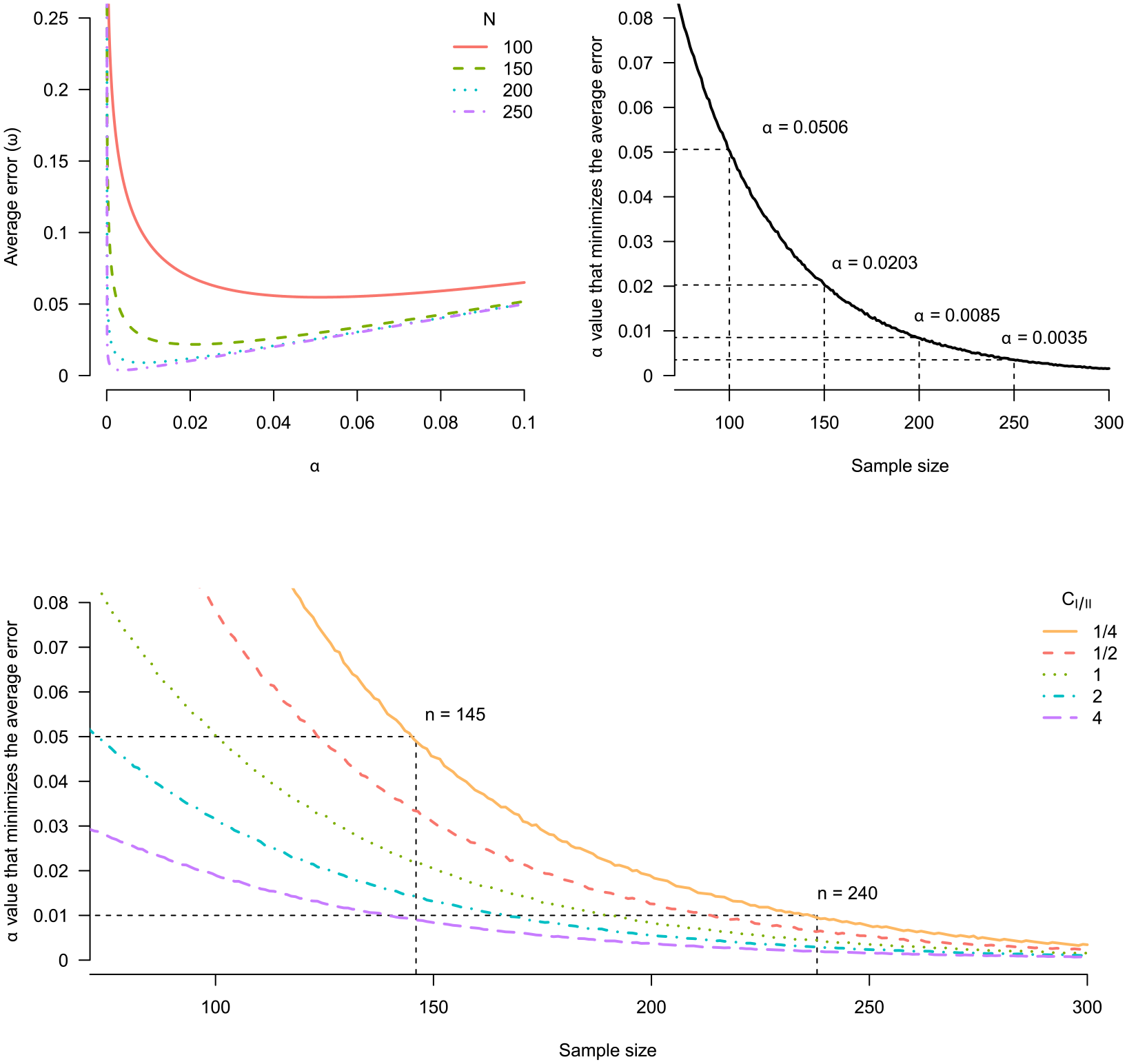
Minimizing the average error for a two-sample, two-sided independent t-test. Upper left: average error ω as a function of α for various sample sizes. Upper right: selecting the α that minimizes the average error as a function of sample size. Bottom: selecting the α that minimizes the average error as a function of sample size for various relative costs of Type I and Type II errors (C I/II ).
As an alternative to minimizing the average error, we can reach a similar conclusion by balancing Type I and Type II errors. The relationship between α and β implies that decreasing α decreases the power (1−β) to detect deviations from the null (Mudge et al., 2012). Since a larger sample size means greater power, using a fixed α across sample sizes means that the Type I probability will often be orders of magnitude larger than the Type II probability. In the limit, the power for all consistent tests tends to 1 as n → ∞; thus, the Type I probability becomes infinitely times larger than the Type II error, making the test severely biased toward Type I errors (Kim et al., 2018).
From Figure 1, we see if n = 100, the power is 94.4% resulting in a Type II error of 5.96% (100 − 94.4). So, by setting α = 0.05, the two error types are relatively balanced. However, for n = 250, the power is 99.99%, 500 times smaller than the Type I error rate 5%. Unless a researcher has a compelling reason, it makes little sense to operate with this kind of error imbalance as a default. Instead, lowering α to 0.35% for n = 250 would still provide power of 99.59% (i.e. β = 0.41%) while making the error rates almost balanced. 2
Unequal costs and priors
In some cases, it may be sensible to use unequal error rates depending on the relative costs of Type I and Type II errors and the base rate of true effects (Miller and Ulrich, 2019). For example, Aguinis et al. (2010) use the relationship between inter-divisional knowledge and invention impact (Miller et al., 2007) to illustrate how a Type I error can be more costly than a Type II error. Falsely concluding that such a relationship exists could lead firms to invest resources into knowledge transfer across divisions without any gains. However, a Type II error results in opportunity costs for firms by missing out on profitable investments. Aguinis et al. (2010) argue that in this case, a Type I error is more costly than a Type II error.
Changing the relative error costs or the base rate of a true effect shifts the optimal α curve, but their effect on the optimal α diminishes as the sample size increases, as shown at the bottom of Figure 1. For example, the orange curve shows a scenario where the cost of making a Type II error is four times that of a Type I error (CI/II = 1/4). Beyond n = 300, the optimal α is almost entirely insensitive to the relative cost of a Type I error to a Type II. Thus, for surprisingly small sample sizes, unless researchers need to work with extremely unequal error costs and/or a very high probability that H1 is true, the relative costs and prior probabilities have almost no influence. This underscores that if we want to minimize or balance the weighted costs, the sample size is the key determining factor.
A Bayesian perspective
Reducing α as the sample size increases is also logical from a Bayesian perspective (Leamer, 1978). The p-value probability distribution function (pdf) is a function of statistical power (Cumming, 2008): higher power results in a more right-skewed distribution. Indeed, as statistical power increases, small p-values can be more likely when there is no true effect (H0) than when there is an effect (H1) (Maier and Lakens, 2022). Figure 2 displays this phenomenon, also known as Lindley’s paradox (Wagenmakers and Ly, 2021). If there is no effect (H0 is true), p-values are distributed uniformly (solid line) irrespective of the sample size. When there is an effect (H1 is true), the p-value pdf becomes skewed, indicated by the dashed lines. Furthermore, a larger sample size produces a more right-skewed distribution since observing small p-values becomes even more likely. For example, if your sample size is very large, you are almost certain to see a very small p-value if there is an effect; thus, if you only see a moderately small p-value, say 0.04, it is quite unlikely that the alternative is true because you would expect to see a p-value much smaller than this.
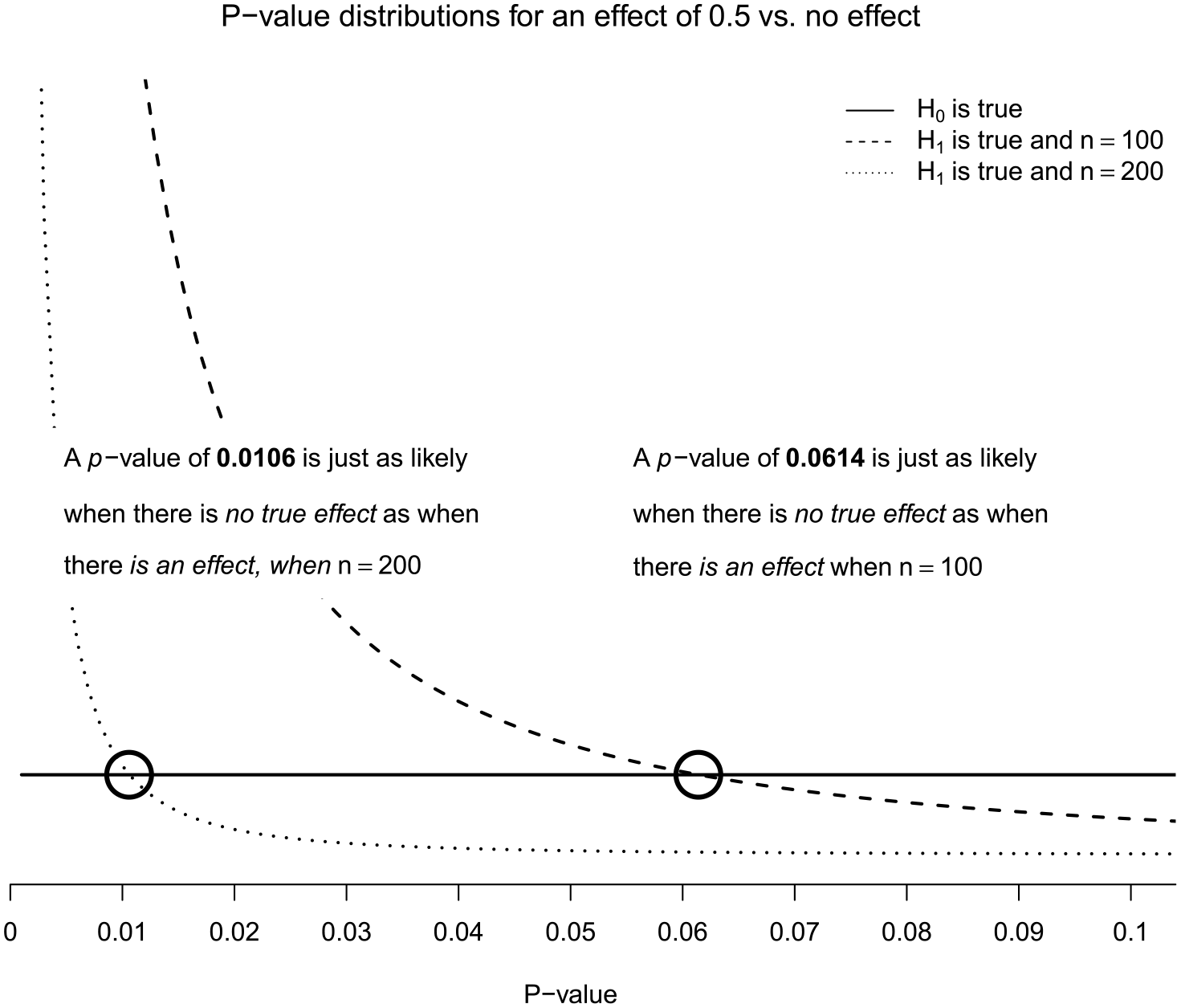
Illustration of Lindley’s paradox. P-value distributions for a two-sample, two-sided independent t-test with n = 100 and n = 200 in each group, respectively, shown for an effect size of 0.5 and of 0 (“no effect,” solid line). The black circles mark which p-value is just as likely to be observed when there is no true effect as when there is an effect.
When the solid line is above the dashed line, the corresponding p-value is more likely to be observed when there is no effect than when there is an effect. The point at which the lines cross (marked by circles) represents the point at which the null and alternative hypotheses are equally likely. As the sample size increases, the p-value at which the null and alternative hypotheses are equally likely decreases. If there are 200 observations in each group (these p-values are from two-sample t-tests), this point is 0.0106, well below the conventional 0.05. So, if the observed p-value is between 0.0106 and 0.05, a researcher using α = 0.05 will reject the H0 even though H0 is more likely than H1. This demonstrates how p-values of a given size do not indicate a fixed level of evidence for the alternative over the null (Royall, 1986).
Existing solutions
The α level is critical to NHST. It is a line drawn in the sand to guide actions while controlling the frequency of mistakes. However, arbitrary fixed thresholds lead to Lindley’s paradox when samples are large. In response, some journals, such as the SMJ, have a submission policy that rules out all thresholds. Instead, authors must report exact p-values, confidence intervals, and effect sizes. Yet, removing all thresholds is unlikely to be a sensible solution (Mayo and Hand, 2022). The core mission of management scholarship is to contribute to management practice (Banks et al., 2016) by shaping what managers do on a day-to-day basis (Aguinis et al., 2022). Ultimately, consumers of management research wish to be informed on whether to take action; to do this, they must set a decision threshold for whether to take action (Schad et al., 2021). Thus, even if journals remove thresholds, it will not stop the need for them.
Reporting only confidence intervals is often seen as a threshold-free alternative to NHST (e.g. Bettis et al., 2016). However, confidence intervals are merely more subtle in introducing thresholds into statistical inference. The width of the confidence interval is directly related to the choice of alpha. A confidence level of 95% implies an alpha of 5%. And so, we are back to the question of this article: How should the alpha level be chosen?
Others still have proposed to lower the conventional α level, for example, to 0.005, at least for new discoveries with low prior odds (Benjamin et al., 2018). Alas, this suggestion misses the root of the problem, which is not the size of alpha, but that it remains fixed across different sample sizes (Lakens et al., 2018a).
Finally, there have been many calls to disregard statistical significance in favor of practical significance (Van Witteloostuijn, 2020). Oftentimes, an effect will be statistically significant but lack any importance in the real world due to its size. We support the drive to shift focus from statistical significance to practical significance but note that, again, it does not negate the need for a threshold. A test for practical significance follows identical logic to statistical significance but with the value under the null shifted from 0 to the SESOI. Thus, we can specify an interval null hypothesis that covers a range of values deemed too small to be meaningful (Murphy and Myors, 1999). For instance, if a researcher was not just interested in whether an effect exists, but also if this effect is substantial, they could specify the null hypothesis as a range of effects too small to matter. Rejecting the null hypothesis would mean the effect was not only statistically significant, but also practically significant (Murphy et al., 2014).
Lowering alpha as a function of the sample size
We have seen that statistical thresholds are useful and reducing this threshold as a function of sample size is sensible. In large samples, a Neyman–Pearson perspective reveals we should trade off power for a lower probability of a Type I error (Wagenmakers and Ly, 2021), while a Bayesian perspective suggests we should lower α to avoid Lindley’s Paradox. As eluded to previously, the two perspectives are closely related: minimizing the average error begins to align Bayesian and Neyman–Pearson testing procedures (Cornfield, 1966; Leamer, 1978). However, minimizing or balancing errors requires the researcher to estimate the statistical power, which includes knowing the effect size (Mudge et al., 2012), and to specify both the relative costs of Type I and Type II errors and the relative probability of the null being true. While each of these parameters is challenging to determine, management researchers may find statistical power to be especially difficult. Indeed, power is rarely discussed in management research (Aguinis et al., 2009) perhaps due to the ubiquity of regression models, for which power is complex to estimate (Scherbaum and Ferreter, 2009).
To simplify the process of setting α, we propose a method that avoids power calculations and only requires researchers to specify the sample size. This approach avoids Lindley’s Paradox by setting alpha such that a significant p-value only occurs when the alternative hypothesis is at least as likely as the null hypothesis (Maier and Lakens, 2022). In most cases, this will also lead to more balanced error rates than when using conventional α values. Indeed, our approach allows for the possibility to guarantee that Type I and Type II errors are equal.
Bayes factors
To set α to avoid Lindley’s Paradox, we connect the p-value to an inference criterion that demands increasing evidence from the data as the sample size increases. One such criterion is the Bayes factor (BF) from Bayesian statistics (Kass and Raftery, 1995). The BF contrasts the probability of observing the data, y, under H0 to the probability of the data under H1
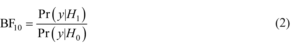
The BF expresses the evidence for H1 relative to H0 in the data, that is, which of the two hypotheses is more likely to have generated the data. Unlike the p-value in equation (1), the BF accounts for both H0 and H1. By weighing the support for one model against the other, the BF quantifies the evidence for and against two competing statistical hypotheses (Andraszewicz et al., 2015). A BF of 1 suggests equal evidence for H0 and H1, while a BF of 10 suggests the data are 10 times more likely under H1. BFs have a continuous scale, but Jeffreys (1939) suggested a series of discrete categories of evidential strength that can be useful to summarize the BF where BFs between 3 and 10 imply moderate evidence, and BFs larger than 10 imply strong evidence (Lee and Wagenmakers, 2013).
While BFs make it possible to quantify the support for one hypothesis relative to another hypothesis, a common pitfall is to interpret BFs in an absolute manner (Wong et al., 2022). For instance, based on a BF of 3 we may conclude that H1 is three times more likely than H0. However, it would be incorrect to draw conclusions like “there is a difference between two groups.” The primary function of the BF is not to endorse binary conclusions but rather to present evidence supporting each hypothesis under scrutiny (Tendeiro et al., 2022).
To derive principled decisions from continuous inferences, one must employ utility functions. Examples of such functions include the Type I and II error rates upon which NHST is founded (Schad et al., 2021). BFs do not directly control error rates, meaning they do not dictate how often an incorrect decision is made (Hoijtink et al., 2019). However, simulations suggest that using a BF > 3 cut-off results in fewer Type I errors compared with a 5% alpha level. This advantage comes at the expense of substantially elevated Type II errors in contrast to the results using NHST (Kelter, 2022). As we explain below this relationship between BFs and error rates can be harnessed to forge a balanced approach that incorporates both controlled error rates and an evidence-based interpretation.
In conclusion, the primary advantage of the BF lies in its capacity for a more intuitive elucidation of scientific evidence. Its limitations, however, include the inability to make binary claims about the existence or absence of effect and the lack of direct error rate control.
Connecting Bayes factors to p-values
The Bayesian-Frequentist compromise we propose combines the evidential aspect of Bayesian statistics with the error control aspect of frequentist statistics. This compromise is achieved by transforming p-values into a BFs, and ensuring α is set such that Lindley’s paradox is avoided.
Several easy-to-calculate bounds for BFs exist; for example,
In this article, we use the approximated adjusted fractional BF (AAFBF) of Gu et al. (2018). The AAFBF is sample-size-dependent and extends to testing hypotheses for regression models. As shown in detail in Appendix 2, for the test of a coefficient in a regression model, the frequentist p-value is connected to the Bayesian BF in the following way
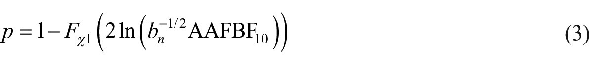
where
Guidance for setting
To set the alpha level as a function of sample size, we need to choose
If researchers wish to be conservative against small effects, there are three options:
One could argue that our method has replaced one arbitrary choice, alpha, with another arbitrary choice,
Examining our choice of α as a function of sample size
Figure 3 illustrates our choice of α as a function of n for various BFs. A close examination reveals three key insights: (1) p-values of a given size do not indicate evidence of fixed strength, (2) α = 0.05 is too high for the most common sample sizes in management, and (3) fixed thresholds are doomed to fail.
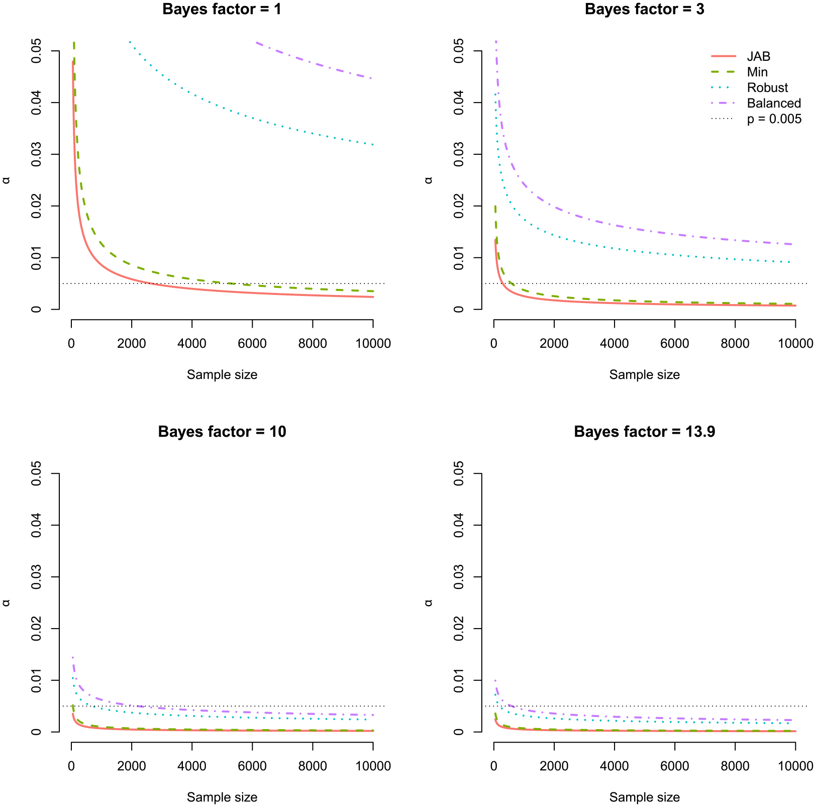
Examining our choice of α as a function of sample size. Each plot illustrates α as a function of n depending on the desired BF: H0 and H1 are equally likely (BF = 1, top left), moderate evidence (BF = 3, top right), strong evidence (BF = 10, bottom left), and the lower BF bound suggested by Benjamin et al. (2018) (BF = 13.9, bottom left).
P-values of a given size do not indicate evidence of fixed strength
Figure 3 illustrates the strong dependence of α on sample size. The larger the sample size, the smaller the p-value corresponding to a given BF. Consequently, a p-value of a given size does not indicate evidence of fixed strength (Royall, 1986). In this light, it is problematic that management researchers rank their results according to which are “highly significant,” “significant,” or just “marginally significant” depending on the p-value (Aguinis et al., 2018) or use the p-value directly as a measure of the strength of a result (Bettis et al., 2016). Instead, the p-value can be viewed as an indirect measure of evidence whose magnitude must be judged in relation to the sample size used to compute it (Hartig and Barraquand, 2022; Lakens, 2022b). For instance, a p-value of 0.002 maps to between moderate and strong evidence for H1 (BFJAB = 3.86, BFbalanced = 28.91) for n = 1000. However, if n = 10 million, the same p-value provides at best anecdotal evidence for H1 (BFbalanced = 2.89) and at worst strong evidence for H0 (BFJAB = 0.04). This demonstrates how p-values are not a consistent measure of evidence (Hubbard and Lindsay, 2008).
The default α = 0.05 is too high
Aguinis et al. (2010) surveyed papers published in Administrative Science Quarterly, AMJ, and SMJ from 2002 to 2006 and found 96% used α = 0.05 to declare a result statistically significant. Assuming a sample size of 800, which was the median sample size reported in 300 management papers published between 2007 and 2016 (Villadsen and Wulff, 2021a), rejecting the null with α = 0.05 would only ensure evidence of between 0.24 (Jeffreys’ approximate BF (JAB)) and 1.76 (balanced); at best, only anecdotal evidence for H1. If researchers instead set α as a function of sample size, they could set α = 0.0029 (for n = 800) to be conservative against small effects (JAB) or α = 0.0258 when Type II errors are costly. This demonstrates how researchers working with median-sized samples risk rejecting the null, even though—in the best case—there is only anecdotal evidence for H1.
Fixed thresholds are doomed to fail
Benjamin et al. (2018) suggested changing the default alpha level to 0.005 for claims of new discoveries. The argument for lowering α to 0.005 was based partly on a Bayesian argument, because, for a two-sided t-test, p = 0.005 implies a large-sample upper bound on the BF between 13.9 and 25.7 (Sellke et al., 2001). However, as argued earlier, the Volke-Sellke bound is limited as it does not depend on the sample size.
In the bottom right of Figure 3, we set the desired level of evidence to 13.9, representing the lowest BF bound used by Benjamin et al. (2018). However, if we want to ensure BF ⩾ 13.9, we require an α smaller than 0.005 whenever n > 587; moreover, this result is based on using
Recommendations and empirical demonstrations
In Table 1, we provide steps to correctly set α organized around the three typical stages of an empirical project: Planning, analysis and reporting. In the planning phase, we recommend researchers consider significance testing if they wish to make scientific claims and decide to take a particular action without being wrong too often (Lakens, 2022a: 1). Researchers should think carefully about the null model. In the organizational sciences, variables frequently exhibit interconnections via causal frameworks, leading to genuine yet theoretically insignificant correlations that lack managerial relevance (Combs, 2010). This phenomenon is referred to as the “crud factor” (Meehl, 1990; Orben and Lakens, 2020). Given the improbability of a zero-effect in extensive correlational datasets, rejecting a nil null hypothesis does not provide a severe test. Even if the hypothesis proves erroneous, it is likely a zero effect will be rejected because of “crud.” Instead of rejecting an effect of zero, researchers can reject a range of values too small to be meaningful by performing a minimum effect test (Murphy and Myors, 1999). A minimum effect test does not distinguish between statistical and practical significance (Lakens, 2022a: 9). The researcher chooses a test value representing the SESOI and when this value is rejected, the effect is both statistically and practically significant (Murphy et al., 2014).
Next, select a method for calculating
With
Here, we apply the proposed Bayesian-frequentist compromise to four published studies. Each study has been selected to demonstrate how researchers may decide on which
Re-analyzing published p-values using a frequentist-Bayesian compromise.
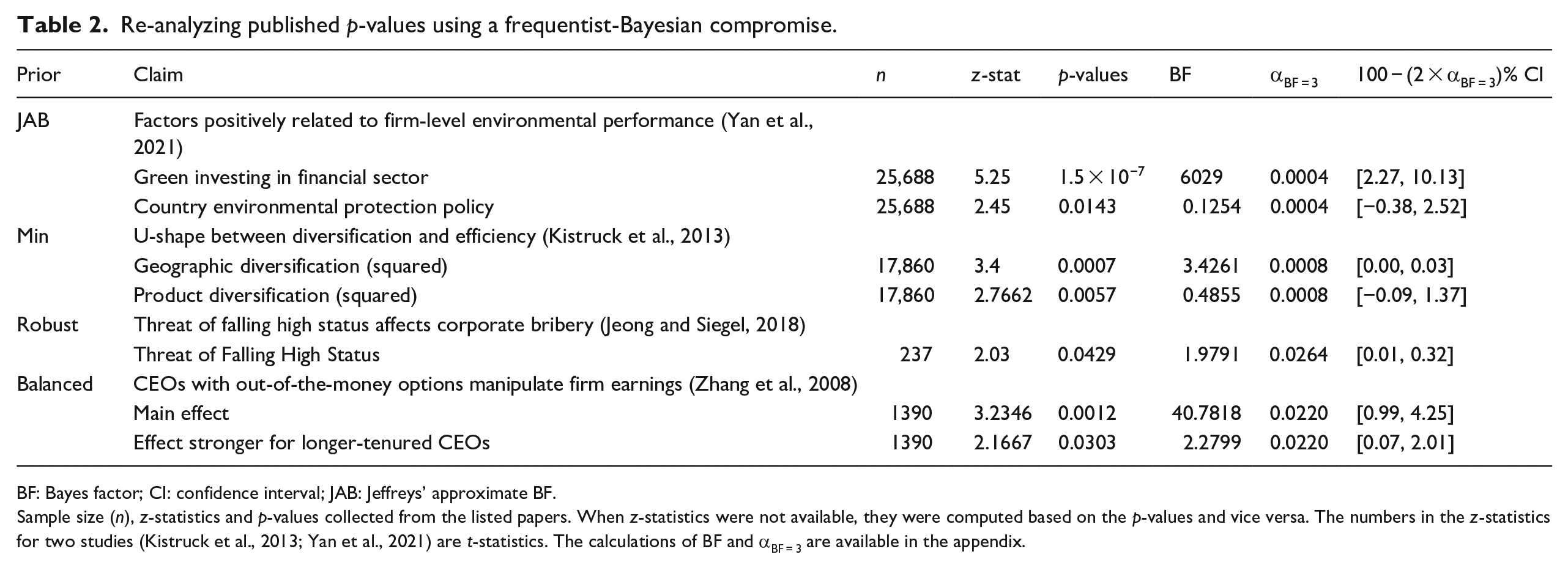
BF: Bayes factor; CI: confidence interval; JAB: Jeffreys’ approximate BF.
Sample size (n), z-statistics and p-values collected from the listed papers. When z-statistics were not available, they were computed based on the p-values and vice versa. The numbers in the z-statistics for two studies (Kistruck et al., 2013; Yan et al., 2021) are t-statistics. The calculations of BF and αBF = 3 are available in the appendix.
Example 1: trivial effects and costly Type I errors
In the first study, we use the JAB prior. This prior is relevant when factors such as measurement error or an observational research design make it highly unlikely that any effect is exactly zero. Yan et al. (2021) collect a large sample of observational data on firms’ environmental performance and regress a subjective environmental score on various factors such as the proportion of green investing in the financial sector. In such a case, it is wise to be cautious of overstating the significance of trivial effects in large sample sizes. The JAB prior is an excellent default to safeguard against trivial findings that might be due to unintended factors, for example, measurement error in grading the environmental performance of firms. Finally, in this situation Type I errors are costly. For instance, if there is no effect of green investing on environmental performance, a false-positive may lead to millions of dollars wasted on green investing. As discussed above, the JAB prior provides the lowest alpha of the four default priors, providing the most protection against Type I errors.
In their original study, Yan et al. (2021) consider p-values lower than 0.1 to be significant. Given their sample size of 25,866, we require α = 0.0004 to achieve moderate evidence. The exact p-value of 1.5 × 10⁻⁷ related to green investing shows their result is still significant if we use the more stringent alpha level. In fact, the BF of 6029 suggests overwhelming evidence for the alternative hypothesis. The authors test a second hypothesis concerning environmental protection policy and report a p-value of 0.0143. This corresponds to a BF of 0.1254, suggesting the null is approximately eight times more likely than the alternative, despite the null being rejected in the original paper. To check whether the effect of green investing is not only statistically significant, but also practically significant, we perform a minimum effect test. For a minimum effect test, we specify a 100 − (2 × 0.0004) = 99.999% confidence interval. For illustrative purposes and simplicity, we set the SESOI to reflect Cohen’s (1988) effect size of 0.05, which is equivalent to a coefficient of 1.615 in a linear regression. 3 Because 1.615 falls outside the 99.999% confidence interval of 2.27 and 10.13 the result is practically significant, and we can claim there is a minimum effect of at least 1.615. At the same time, we can conclude that it is at least 3 times more likely that there is a meaningful effect than not.
In sum, the authors could have provided more impressive support for their hypothesis regarding green investing while avoiding claiming a significant effect for environmental protection policy in the face of substantial evidence to the contrary.
Example 2: large-sample likelihood misspecification
For the second study, we use
Kistruck et al. (2013) hypothesize a u-shaped relationship between efficiency and two types of diversification. A sample size of 17,860 requires α = 0.0008 to achieve at least moderate evidence with a minimum training sample prior. Letting alpha depend on the sample size would have allowed Kistruck et al. (2013) to provide more impressive support for their hypothesis regarding geographic diversification where the alternative is at least three times more likely than the null. With respect to product diversification, our approach suggests that despite the significant result found in their paper (p = 0.0057), it is actually more than twice as likely that the null is true compared with the alternative (BF = 2.0597).
Example 3: small-sample likelihood misspecification
In the third example, we use
The article’s main result gives a “significant” p-value of 0.0429 for the effect of the threat of falling high status. However, using the robust prior, we should set α = 0.0264 to achieve at least moderate evidence. Thus, there is less than moderate evidence for the alternative (BF = 1.9791). This insignificant result does not give conclusive evidence of no effect (Lakens et al., 2020), it suggests that more data is needed to conclude whether the threat of falling high status is indeed a determinant of large-scale corporate bribery.
Jeong and Siegel (2018) rely on a panel consisting of 40 business groups of which 39 are observed for the full period of 6 years. Because bribe amounts paid by a business group are likely correlated across years, the effective sample size is likely smaller than 237. Although we do not have access to the data used in the study, we can perform an imaginary post-analysis check: Imagine that running the regression in the article with regular standard errors would have resulted in a standard error twice as large as the reported clustered standard error. In this case, we would need to use an effective sample size four times (22 = 4) smaller, about 59. This would result in α = 0.0396, which still gives an insignificant result when compared with the p-value of 0.0429. In other words, we cannot claim an effect even if we imagine the effective sample size to be four times smaller than the total number of observations.
Example 4: costly Type II errors
Finally, Zhang et al. (2008) investigate whether CEOs with out-of-the-money options manipulate firm earnings. In this case, a prior that balances the error rates would be a wise choice since a Type II error could be costly. Not detecting such behavior could cause serious problems: stock price decline, reputational damage, top management turnover, possible bankruptcies, and loss of investor confidence (Aguinis et al., 2010).
The study uses a sample of 1390, so we set α = 0.0220 to achieve at least moderate evidence. At this level, we still find a significant relationship (p = 0.0012) with strong evidence (BF = 40.7817). If the authors had set their alpha to achieve at least moderate evidence, they could have presented stronger support for their main claim without being too concerned about a Type II error. To their surprise, Zhang et al. (2008) find that longer-tenured CEOs with greater value in out-of-the-money options are more likely to manipulate earnings (p = 0.0303). However, our re-analysis suggests this result is insignificant and only provides anecdotal evidence (BF = 2.2799). If the authors had set α to achieve at least moderate evidence, they could have presented stronger support for their main claim while avoiding interpreting a surprising result as anything more than anecdotal.
Discussion
There is significant debate on significance testing and p-values, particularly in light of the replication crisis. Indeed, many scientists have argued that significance tests should be abandoned altogether (Anderson et al., 2000; Carver, 1993; Gill, 1999). This view has been echoed in management research, where some recommend we “let go of statistical significance once and for all” (Van Witteloostuijn, 2020: 275), “escape the straightjacket of NHST” (Lockett et al., 2014: 870), “stop relying on NHSTs” (Schwab et al., 2011: 1106), or even that “[i]t would be better for journals to ban p-values as well” (Starbuck, 2016: 74). The misinterpretation of p-values has lead SMJ to no longer accept papers “that report or refer to cut-off levels of statistical significance” (Bettis et al., 2016: 261), and other journals, such as Management and Organization Review, to conclude that “the use of cut-off level of p-values to support or reject hypotheses is inappropriate” (Li et al., 2017: 440).
We agree that significance testing is often misused, but this does not warrant abandoning it; abusus non tollit usum—or, abuse does not cancel use (Mudge et al., 2012). If all misused tools were abandoned, there would be few left to use; indeed, confidence intervals are often misinterpreted (Greenland et al., 2016), and Bayesian methods are frequently misapplied due to incomplete prior reporting (Van de Schoot et al., 2017) or BF misinterpretation (Tendeiro et al., 2022; Wong et al., 2022). Moreover, there are many potential costs if NHST were abandoned (Lakens, 2021): authors might overstate their conclusions more than with NHST, as seen after the 2016 ban of inferential statistics in Basic and Applied Social Psychology (Fricker et al., 2019); without a threshold, there is no test of a claim (Mayo and Hand, 2022); error control is lost (Mayo, 2018); and, NHST is one of the most studied and best-understood statistical procedures (Benjamini et al., 2021).
We support the advice of the President’s Task Force appointed by the board of the American Statistical Association: “P-values and significance testing, properly applied and interpreted, are important tools that should not be abandoned” (Benjamini et al., 2021: 1024). This entails, among other things, justifying the alpha level. Editors stress that researchers take n into account when evaluating statistical tests (Bettis et al., 2016; Combs, 2010; Hahn and Ang, 2017; Meyer et al., 2017), but provide no guidance on how. If researchers look toward standard textbooks in statistics, they will find little help there either:
Elementary statistics texts are not equipped to go into the matter; advanced texts are too preoccupied with the latest and fanciest statistical techniques to have space for anything so elementary. Thus the justifications for critical levels that are commonly offered are flimsy, superficial, and badly outdated. (Bross, 1971)
Our approach is a compromise between Bayesian and frequentist statistics; as with all compromises, we give up some benefits of each. These “pure” approaches might be attractive if researchers are comfortable providing more details, for example, by specifying relative costs of errors or informative priors. A pure frequentist approach is advisable when researchers (1) can specify the relative cost of Type I and Type II errors, (2) can justify the prior probabilities of H0 and H1, and (3) have enough information to perform a power analysis (Maier and Lakens, 2022). A frequentist approach is also recommended when researchers care only about controlling long-run error rates and not about an evidential interpretation of their test (Mudge et al., 2012). However, as demonstrated, a pure frequentist approach that balances error rates will also reduce alpha as n increases, so will often avoid Lindley’s paradox too (Maier and Lakens, 2022).
A fully Bayesian approach is advisable when researchers (1) are comfortable specifying priors for their model parameters, (2) have well-specified alternatives, and (3) accept the computational burden from sampling from the posterior distribution (Harvey, 2017). Hypothesis testing using BFs provides an intuitive evidence-based interpretation, but BFs should not be used for binary decision-making and they do not come with long-run error guarantees (Hoijtink et al., 2019). In Bayesian analyses, to make decisions, one must implement Bayesian decision-making processes (Gelman et al., 2014: 9). These processes transform inferential information, like the continuous Bayes factor or posterior model probabilities, into discrete decisions. Like the “pure” frequentist approach, Bayesian decision-making requires researchers to specify the costs and benefits of decision options under uncertainty and appropriate specification is often challenging (Schad et al., 2021).
There are strong norms to use fixed alpha levels in the management discipline. With this article, we hope to persuade scholars to abandon fixed alphas and instead justify alpha as a function of sample size. Our explanations, demonstrations, empirical examples, and R-package hopefully make this adoption as straightforward as possible.
Footnotes
Appendix 1
Appendix 2
Appendix 3
Appendix 4
Acknowledgements
The authors wish to thank Editor Oliver Alexy and the reviewers for their guidance. The authors also gratefully acknowledge feedback on earlier versions of this article from Daniël Lakens, Maximillian Maier, Eric-Jan Wagenmakers, and attendees of the 2023 Annual Meeting of the Academy of Management in Boston and the Organization, Strategy and Accounting (OSA) seminar at the Department of Management, Aarhus University.
Funding
The author(s) received no financial support for the research, authorship, and/or publication of this article.
Data availability
The R-package is available on GitHub (https://github.com/jespernwulff/alphaN) and has been published on CRAN (https://cran.r-project.org/web/packages/alphaN/index.html). The Shiny web app is available here: ![]() .
.
Notes
Author biographies
Jesper N Wulff is an Associate Professor at the Department of Economics and Business Economics, Aarhus University. His primary research interest lies in quantitative research methods, with a particular focus on enhancing researchers’ understanding and use of statistics. While his main emphasis is on addressing applied statistical challenges within the realm of management research, he also contributes his expertise as a statistician to empirical studies spanning corporate finance, social epidemiology, and public administration.
Luke Taylor is an Associate Professor at the Department of Economics and Business Economics, Aarhus University. His research interests cover two broad areas: (1) theoretical work on nonparametric estimation and testing in the presence of measurement error, and (2) applied work on decision-making in the criminal justice system.