
Abstract
This article presents a multi-physical crack monitoring approach for prestressed concrete girders, combining ultrasonic pulse velocity (UPV), acoustic emission (AE), and strain measurement by distributed fiber optic sensors (DFOS) within a cyclic loading scheme. The proposed approach was applied to a prestressed concrete girder extracted from a decommissioned bridge built in 1981. The results demonstrated the strength of this multi-physical approach for monitoring a broad spectrum of crack behaviors in prestressed concrete structures. It can identify existing cracks with minimal loading. The applied load levels were below the estimated decompression force. Additionally, the approach can distinguish between the formation of new cracks and the growth of existing ones. Notably, the formation of new cracks led to a more significant reduction in local stiffness, as indicated by the force and DFOS strain measurements. Furthermore, a potential relationship was observed between the AE hit rate and the DFOS strain rate during the formation of new cracks. Moreover, this approach enabled detection of possible damage inside the structure such as at the interface between the cast-in situ overlay and the precast girders or in the internal web. This study contributes to the development of more comprehensive monitoring strategies for aging prestressed concrete structures.
Keywords
Introduction
Most transportation infrastructure, such as bridges and tunnels, is built with concrete. 1 Among them, an important type of structure is a prestressed concrete girder. 2 A large proportion of prestressed concrete bridges in Western Europe was constructed between the 1960s and 1980s. 3 Over time, deterioration of material, increased traffic loads, and dated structural designs that may no longer meet current code requirements have raised concerns regarding the safety of these structures. 4 Consequently, there is a pressing need for effective assessment of existing prestressed concrete structures.
Cracking behavior in the prestressed girders is an important indicator of the health condition of the structure. The causes of the cracks could be unexpected overloading of the structure in its service life or local distressing of the structure due to unwanted deterioration mechanisms. 5 For instance, in the assessment of the prestressed bridges at risk of stress corrosion cracking (SCC), 6 cracks that open later in the life of the structure and whose crack growth accelerates can be important indicators of tendon damage.
By detecting the presence of existing cracks and monitoring the opening of new cracks, timely decisions can be made regarding the optimum intervention strategies. 7 Such monitoring-informed decisions not only ensure structural safety 8 but also offer economic benefits by reducing costs associated with unnecessary repairs, traffic restrictions, or complete bridge replacements.9–11
Various techniques are available for crack monitoring or detection in prestressed concrete. The conventional method is visual inspection, which is often subjective, with limited reproducibility, only applies to crack detection on the structural surface, requires traffic restrictions, and leads to high costs when applied with short time intervals. In recent years, advancements in technology have led to several non-destructive techniques for crack monitoring or detection, which could be vibration-based, 12 image-based such as digital image correlation (DIC), 13 elastic wave-based such as UPV, 14 elastic wave tomography, 15 coda wave interferometry (CWI),16,17 acoustic emission (AE) monitoring, 18 and optical fiber-based such as distributed fiber optic sensors (DFOS).19–21
Recent studies have explored the integration of multiple sensing techniques to enhance crack monitoring. For example, CWI has been paired with vibration monitoring, 22 where vibration monitoring verified the CWI for crack identification. DFOS has been integrated with DIC, 23 using DIC to validate the crack location and width detected by various types of DFOS. AE has been combined with DIC,24,25 with AE providing insights into internal cracking while DIC provides precise surface measurements. These multi-physical approaches allowed different techniques to cross-validate and complement each other.
However, crack monitoring and detection in prestressed concrete structures remain significantly challenging due to the complex structural configuration and stress distribution. One difficulty is that newly formed cracks in prestressed girders tend to have extremely small widths, 25 requiring sensitive detection methods. Additionally, once the external load is removed, the existing cracks tend to close tightly due to prestressing, making them harder to identify. Furthermore, many prestressed girders incorporate cast-in situ overlays, which are prone to interface cracking 26 that is difficult to detect from the structural surface.
To overcome these challenges, a favorable crack monitoring system for prestressed concrete should have the following capabilities: high sensitivity to concrete cracking, accurate measurement of crack location and width, differentiation between existing and new cracks, and identification of internal damage not visible on the surface. However, according to the literature, no existing technique or combined approach fully meets these requirements.
This paper presents a multi-physical approach within a cyclic loading scheme to enhance the monitoring of complex cracking behaviors in prestressed concrete. The approach integrates three advanced techniques, which are DFOS, AE, and UPV, whose distinct working principles complement each other. Unlike other combined approaches, these techniques are strategically integrated at optimal moments within the cyclic loading scheme to maximize effectiveness. The scheme requires only a light load, which remains below the decompression force, not requiring expensive heavy trucks and ensuring no additional cracks are induced. It shall also be noted that the term “monitoring” in the proposed approach refers specifically to tracking structural performance during the required load tests, rather than long-term structural health monitoring over the service life of the structure.
The method was validated on load testing of an 11-m prestressed concrete girder extracted from a real bridge built in 1981. The realistic structural configuration, material properties, and possible pre-existing cracks make the test a valuable case study. The results confirm the effectiveness of the proposed approach in crack monitoring in prestressed concrete and provide scientific insights into potential correlations among the underlying physics.
The remainder of this article is organized as follows: the second section provides an overview of the techniques of UPV, AE, and DFOS, including their working principles and capabilities in crack monitoring. The third section introduces the proposed approach that combines these three techniques. The fourth section describes the case study where the combined approach is applied. The results of the combined crack monitoring approach are presented in the fifth section. A discussion on the performance of the approach and the future work is provided in the sixth section. Finally, the seventh section concludes this paper.
Overview of the monitoring techniques UPV, AE, and DFOS
Ultrasonic pulse velocity
UPV detects the presence of cracks. In a typical UPV measurement, one transducer sends ultrasonic signals into concrete, and the other transducer receives the signals. A ray path is built between the two transducers. From wave propagation distance and time, UPV calculates the (averaged) wave velocity in the ray path. Cracks in the ray path will delay the wave travel time, resulting in a lower averaged wave velocity.27,28 Moreover, cracks will also reduce the signal amplitude. Some studies use the amplitude drop to identify existing cracks.27,29 By analyzing the wave velocity and the amplitude drop, UPV can detect the presence of existing cracks both on the structural surface or inside the structure.
The resolution of UPV is limited by the sensor placement. When two sensors are placed with a distance larger than the crack spacing, more than one crack would be present in a ray path. In this case, UPV is not able to distinguish the multiple cracks. Even in the advanced methods of tomography, the resolution is not much improved. 30 Moreover, a consistent link is not found between UPV results (either wave velocity or amplitude drop) and crack magnitude.28,31,32
AE monitoring
Sudden changes in concrete will release energy and generate AEs. These emissions will propagate in the form of elastic waves in the concrete medium and can be detected by AE sensors. By processing the received signals, one can identify the crack location (which is called source localization 33 ), distinguish different types of sources (which is called source classification 34 ), and determine the structural integrity. 35 AE is sensitive to the formation of new cracks, even microcracking. Therefore, it can detect concrete cracking at an early stage.25,36 Moreover, AE can monitor internal damaging processes, such as wire breaks. 37
A drawback of AE monitoring in concrete structures is its low accuracy of source localization due to multiple sources of uncertainties, such as arrival time picking error, sensor placement error, and the influence of existing cracks.38–40 According to a previous study, the source localization error can reach around 15 cm for a two-dimensional (2D) localization setup. 40 Though AE is sensitive to the location of the cracks, its link to crack width is not trivial.35,41,42 A recent study shows that AE events are not only related to the crack width but also related to the complete crack kinematics, including crack width and shear displacement. 43
Distributed strain sensing with fiber optic sensors
DFOS based on Rayleigh backscattering uses the inherent scattering of light within an optical fiber to measure strain and temperature changes along the entire fiber length.44–47 Rayleigh-based fiber optic sensing is able to measure strain continuously along the length of the fiber with a high spatial resolution in the millimeter range.45,48–50 It enables early crack identification, often before cracks become visible to the human eye.51,52 A recent study shows that DFOS can detect µs less than 0.01 mm.23,53,54 DFOS can also detect the closure of existing cracks through local negative strain peaks. 55 However, the differentiation of existing cracks reopening from newly forming cracks is still a challenge. 56
The choice of DFOS type (considering strain transfer, robustness against chemical and mechanical influences) and the installation method have a major impact on the success of the measurements.20,23 Inadequate DFOS selection or installation results in lower data quality. For example, exceeding the technical limitations of the interrogator results in dropouts (missing values) and strain reading anomalies (SRAs), that is, implausible values. These disturbances complicate the interpretation of the strain signal and need to be dealt with accordingly.57,58 Herbers et al. 59 proposed a methodology for DFOS selection.
Table 1 summarizes the strengths and limitations of the techniques of UPV, AE, and DFOS with respect to the crack monitoring requirements for prestressed concrete structures. The information presented in Table 1 is based on findings from existing literature and does not include the new insights gained from the case study discussed in this paper. According to the literature, individually, none of these techniques fully satisfies all the crack monitoring requirements.
Overview of the capabilities of UPV, AE, and DFOS for concrete crack monitoring.
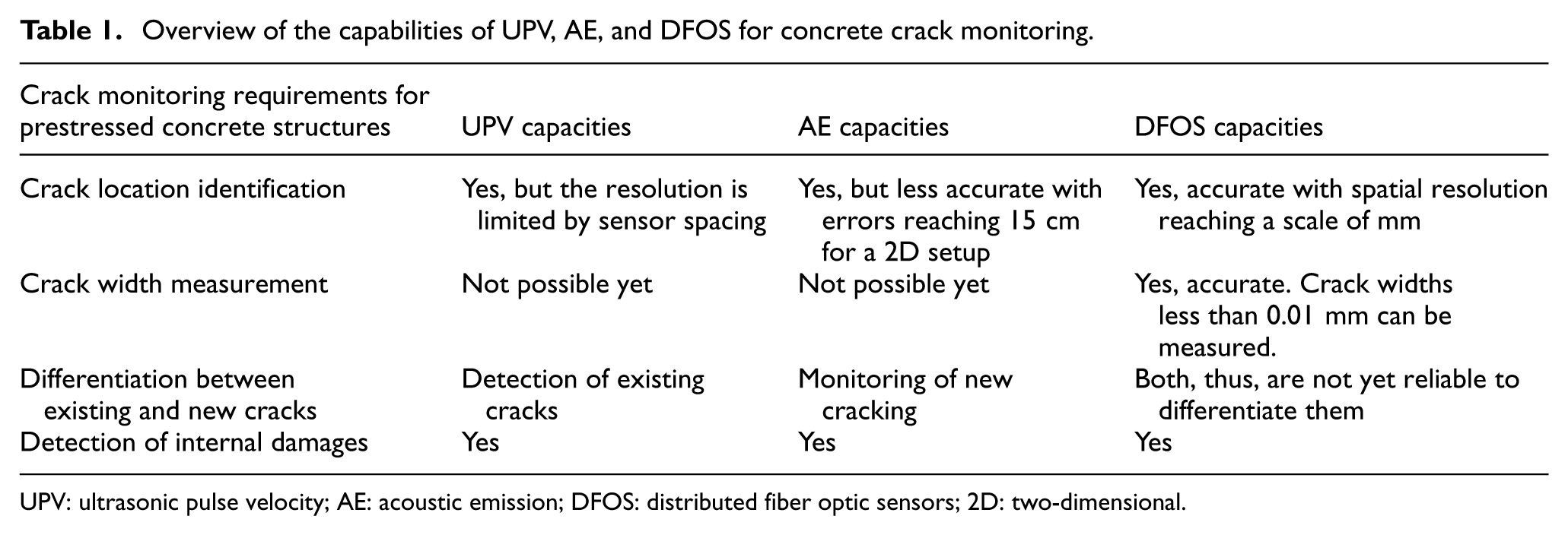
UPV: ultrasonic pulse velocity; AE: acoustic emission; DFOS: distributed fiber optic sensors; 2D: two-dimensional.
A multi-physical approach for crack monitoring in a cyclic load scheme
Based on the strengths and limitation of the techniques reviewed in the second section, a multi-physical approach within a cyclic loading scheme is proposed to monitor the concrete cracking in prestressed girders. The key in the combination is to take advantage of each technique: DFOS accurately measures the crack location, change of crack width, and strain; UPV can detect existing cracks actively without the need for loading; and AE is sensitive and straightforward to indicate new crack opening. Each technique is applied at an optimal stage in the cyclic loading scheme to maximize the effectiveness.
Design of the cyclic load scheme for the combined approach
The designed cyclic loading scheme is compliant with the established guidelines on load testing.60,61 In a load cycle, when first reaching a higher load level, the load is suggested to be held for a while. This hold period serves two purposes: the first is to allow cracking activities to be stabilized; the second is to provide a suitable period for data analysis.
The required load level is minimal, which is lower than the decompression force. At this stage, the first flexural crack would not form at its critical moment cross-section. Estimation of the decompression force requires information of the girder geometry, the prestress force, and the material properties. 62 Then, depending on the objective of the test and the result of the first load cycle, more load levels can be designed.
Figure 1 illustrates the suggested cyclic load scheme. Three stages are suggested: stage 1 is before the load testing, stage 2 refers to the low-load cycle before reaching the decompression force, and stage 3 is when new cracks would form, and existing cracks would grow. Stage 3 is optional and can be modified depending on the objective of the load test.
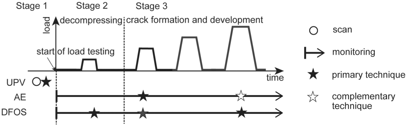
Illustration of the combined monitoring approach using UPV, AE, and DFOS to detect concrete cracking. Three stages of load testing are divided. The circle represents the scanning of the existing cracks, the arrows show monitoring from the start of the load testing, the black star shows the primary technique applied in each stage, and the white star shows the complementary technique. UPV: ultrasonic pulse velocity; AE: acoustic emission; DFOS: distributed fiber optic sensors.
Corresponding to the three stages, the combined monitoring approach is also shown in Figure 1. The circle indicates scanning of existing cracks using UPV. The arrows from the start of the load test indicate the continuous monitoring, which uses AE and DFOS. The black star shows the primary technique that works for each stage, and the white star shows the complementary technique.
Stage 1: Before loading
The first purpose of this stage is to measure the wave velocity in uncracked concrete, which serves as a reference for comparison. In literature, the velocity in uncracked concrete is found empirically to be above 3500 m/s. 63 However, since the wave velocity is related to material properties, 64 it is recommended to measure the wave velocity for the structure under investigation. One can select a surface area on the structure where a crack is not observed or expected to establish a reference velocity.
The second purpose of this stage is to detect the possibly existing cracks in the structure. Measurement could be performed in the critical zones of the structure, such as the zone with the maximum bending moment or the interface between the cast-in situ layer and the precast girder. A reduction of wave velocity is expected if a crack is present and not fully closed in the ray path between the source and the receiver. 65 This article assumes that the pre-existing cracks are not fully closed during UPV tests, due to the inherent roughness and mismatch between crack surfaces.
It is important to note that the use of wave velocity for crack detection is primarily based on studies in the literature, which were conducted on reinforced concrete. In prestressed concrete, a study has reported that the wave velocity would be 2–3% higher than that in reinforced concrete. 14 Given this minor variation, this paper considers the reinforced concrete velocity values applicable and adopts them without additional validation.
Stage 2: At a low-load cycle below decompression force
The main purpose is to verify the existence of cracks detected by UPV in the previous stage. The low-load level is below the estimated decompression force. With the low load level, the existing cracks will be less compressed or reopen. DFOS can accurately measure the local strain peaks at the location of existing cracks. The precise location measured by DFOS can compensate for the low accuracy of UPV. Due to its high accuracy and sensitivity, DFOS is used as the primary technique to identify the existing cracks when a low load is applied.
AE was used to verify existing cracks by monitoring AE events associated with crack closure in reinforced concrete. 66 However, in prestressed concrete, the reopening of the existing cracks at this low-load level would be limited, giving little closure activity. Therefore, the applicability of AE during unloading in the low-load cycle needs to be verified for prestressed concrete.
Stage 3: At higher-load cycles (optional)
As the load increases, the combined approach uses DFOS and AE to track crack formation and development. When a new crack forms, DFOS strain measurements, in conjunction with load data, indicate a reduction in stiffness. However, distinguishing between stiffness loss due to new crack formation and the growth of existing cracks is vital. AE, which detects energy emissions from cracking, provides a more direct and sensitive indication of new crack initiation, including microcracking. By integrating DFOS and AE, the approach ensures more reliable identification of new crack formation.
As cracking progresses and the number of cracks increases, the accuracy of AE source localization declines due to complex wave interactions. Therefore, rather than pinpointing individual cracks, AE analysis is conducted on a zonal basis. Meanwhile, DFOS serves as the primary technique for precise crack localization and width measurement, given its high spatial resolution.
Description of the case study
Bridge girder
The bridge girder under investigation was a prestressed prefabricated element and was part of an agricultural bridge across the highway A24 near Stolpe in north-eastern Germany (Figure 2(a)). This bridge is representative of many bridges that were built in a comparable design in the former German Democratic Republic. After the Second World War, a design series was developed that focused on standardizing bridges with short to medium spans. The aim was the efficient use of the scarce building material at that time. As a result, these prefabricated structures shaped the appearance of the East German bridge landscape for a long time until today.
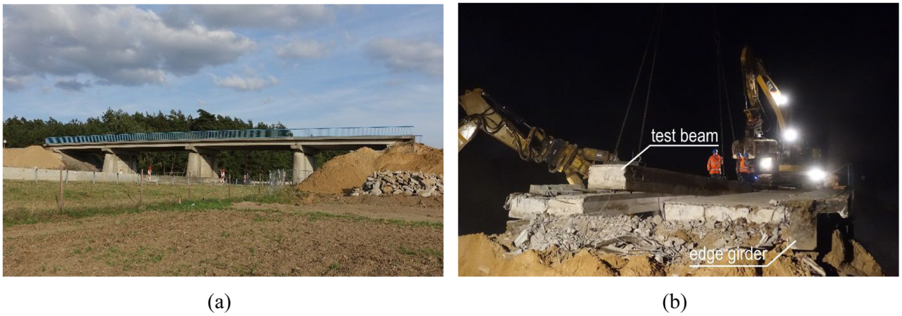
(a) The bridge before demolition and (b) extraction of the test beam during demolition.
The bridge, built in 1981, was designed as four single-span beams. Each span was composed of six adjacent girders of the type BT500N-11,0/2-30 and two laterally placed edge beams. The girders were joined to one slab through a reinforced **in situ concrete layer. The edge beams were additionally secured by horizontal anchors. Each precast element was prestressed by two BSG-50 tendons with 16 wires. The wires were ribbed, oval, and tempered prestressing steel St140/160, which at that time was produced exclusively in a steel plant in Hennigsdorf and was classified as particularly susceptible to SCC. 67 The risk of SCC was the key reason for the deconstruction of the bridge.
A total of three girders were investigated regarding this problem (Figure 2(b)). One of these girders was subjected to a load test, which is presented in this paper. The other two girders were subject to investigations regarding the detection of wire breaks using AE 68 or the analysis of the material properties.
The concrete material properties were studied from a total of 24 drill cores with a diameter of 100 mm. The mean values for compressive strength fcm, tensile strength fct,sp, and elastic modulus Ecm of the concrete were 96.9, 5.54, and 35,500 N/mm2, respectively. It is particularly noteworthy that the results of the tests for compressive and tensile strength of concrete clearly exceed the normative specifications of a B600 (fck = 60 N/mm2, fBz = 3.6 N/mm2) according to the German guideline. 67 The tensile strength of the prestressing steel R m was tested on 19 samples, giving a mean value of 1597 N/mm2. The residual pre-strain was determined based on the static calculation for this type of tendon. 69 It specifies a nominal prestressing force of 483.5 kN. The cross-sectional area of the prestressing steel per tendon containing 16 wires is 560 mm2. Considering an elastic modulus of 205,000 N/mm2 and a prestress loss of 10% due to creep and shrinkage by the time of load testing, the residual pre-strain is therefore estimated to be 3.79‰.
Determination of relevant load situations
The beam was subjected to a four-point bending test at the test facility at the University of Applied Sciences in Wismar (Figure 3(a)). The main span was set to 10.5 m. Two hydraulic jacks were used to apply the load, with each at a distance of 3.75 m from the support axes. The spacing between the two hydraulic jacks was 3.0 m. The purpose of this load testing setup was to expose a considerable segment of the beam to a constant moment, enabling the investigation of crack formation and propagation.
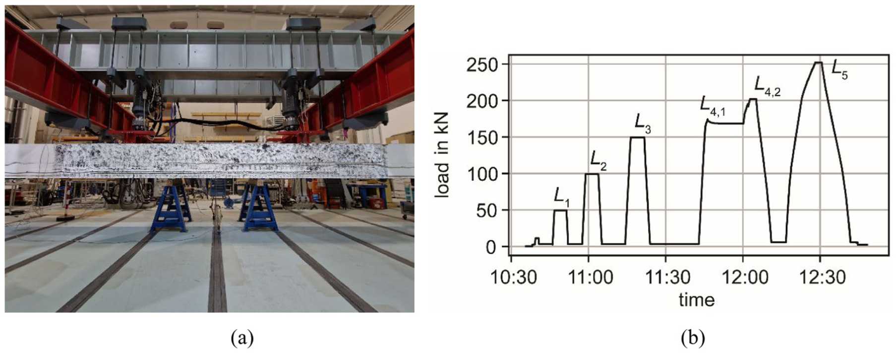
(a) Prestressed girder in the test facility and (b) the cyclic loading scheme.
To determine the loading scheme and to calculate when the girder will transition to the crack formation stage, calculations were first carried out based on the material parameters presented in “Bridge girder” section. Assuming linear-elastic material behavior, concrete strains εc,b at the bottom of the girder can be determined as follows:
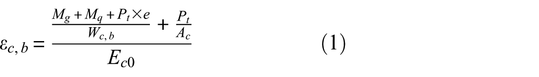
where M g = 140 kN·m is the bending moment in the midspan due to dead weight, M q is the bending moment due to the applied load F, P t is the existing prestressing force, e is the distance between the center of gravity of the cross-section and the tendon axis, Wc,b is the section modulus, A c the geometric cross-sectional area, and E c ,0 the initial tangent modulus of the concrete, with E c ,0 = 1.1 × Ecm.
The residual pre-strain in the strands was assumed to be 3.8‰ according to “Bridge girder” section, which corresponds to a residual stress of 781 N/mm2. The tendons are assumed to be fully intact, which is an assumption supported by the experiments where the tendons were exposed, and the wires were cut. Through calculation, the decompression state is reached at F = 84 kN, when εc,b = 0‰. The theoretical cracking force is Fcr = 183 kN, when the ultimate concrete strain is reached εc,b = 0.1‰. And the steel yielding starts theoretically at F y = 330 kN.
Loading scheme
Figure 3(b) shows the cyclic loading scheme where five load cycles were applied. The load was applied in force control except for the load levels of L4,1 and L4,2. According to the determination of the load situations in “Determination of relevant load situations” section, at the load level L1 = 50 kN, the girder was expected to be at the stage of decompressing. A new crack formation was not expected. Then, in the subsequent load cycles, the girder was loaded with an additional 50 kN in each cycle, with an intermediate load level L4,1 in the fourth load cycle. Since the girder was to be used for further studies on SCC, the load was limited to a maximum of 250 kN to avoid steel yielding.
Measurement setup
Figure 4 shows the measurement setup. Among all the measurements, DIC, inclinometers, and linear variable differential transformers (LVDTs) for deformation were not used for this study. Therefore, only the relevant measurements to this paper are introduced, which include:
Load measurement using load cells on the hydraulic jacks,
Deflection measurement using LVDTs at the midspan of the girder,
UPV tests at local positions on the top and bottom surface, across the girder height, and in the bending and shear zones,
AE monitoring in the bending and shear zones, and
DFOS strain measurement on the bottom surface along the girder.
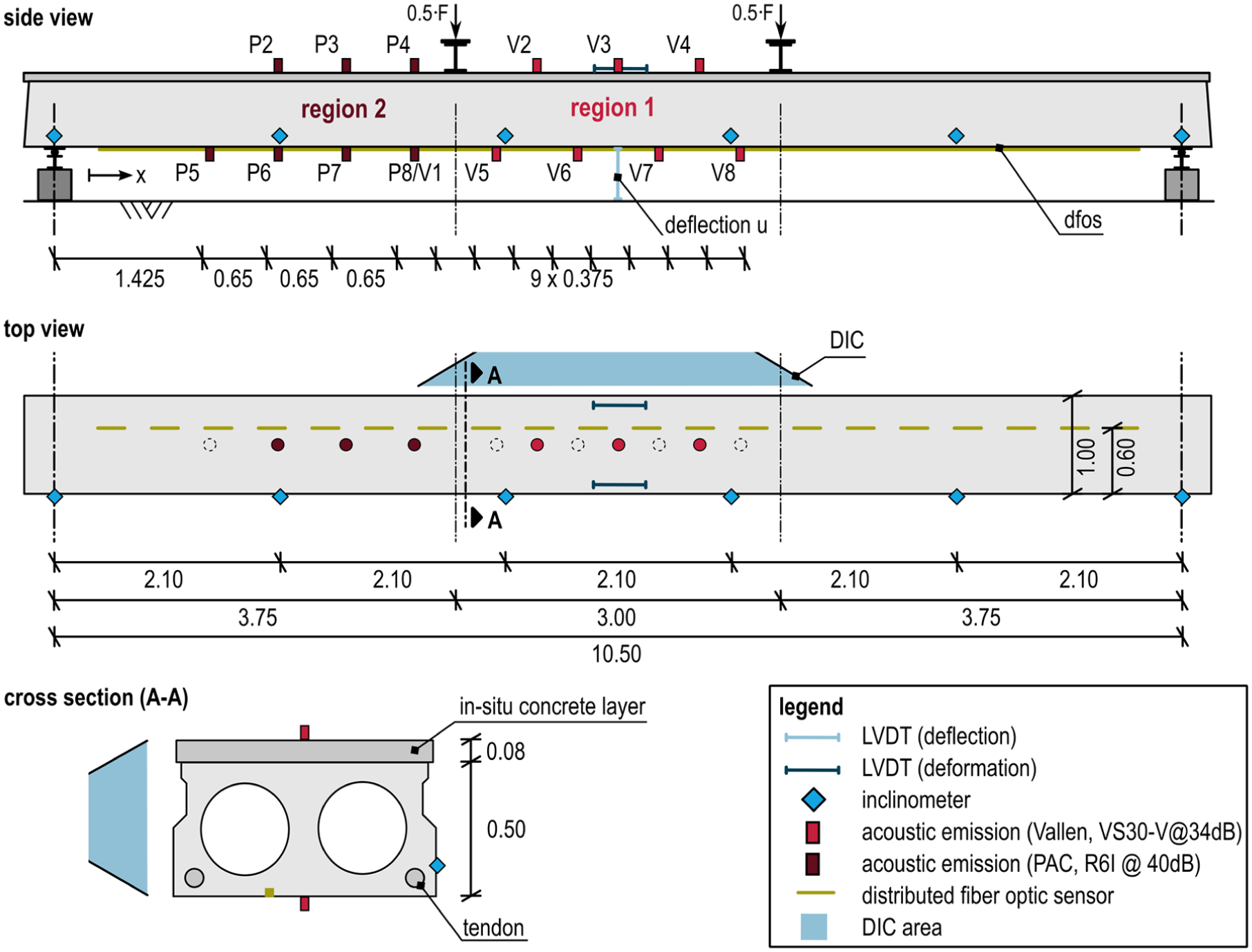
Layout of the applied sensors including LVDTs, inclinometers, AE sensors from two different fabricators, that is, Vallen and PAC, DFOS, and DIC. LVDT: linear variable differential transformer; AE: acoustic emission; DFOS: distributed fiber optic sensors; DIC: digital image correlation.
Ultrasonic pulse velocity
UPV tests used the AE sensors from the two fabricators, that is, Vallen and physical acoustics corporation (PAC). They can serve for UPV purposes because as a type of piezoelectric transducer, the AE sensors cannot only receive signals but also send signals as sources.
Before installing the sensors, the concrete surface was ground and cleaned for a better coupling effect. The sensors were coupled to the concrete surface with hot-melt glue. No additional mounting device was used (Figure 5(b)).

Measurement of wave propagation properties on the structural surface using pencil lead break tests: (a) sensor location and pencil lead break location, (b) installation of sensors on the top surface, and (c) installation of sensors on the bottom surface.
UPV test setup
UPV tests were performed to identify the existing cracks before the load testing. Three different test setups were used, with sensors placed in different regions. Detailed descriptions of the test setups of each UPV test are provided below.
Test 1: Measurement of velocity in uncracked concrete
UPV test 1 was performed at the top and bottom surfaces of the girder, where no crack was observed, including three measuring locations (Figure 5(a)). The purpose is to measure the wave propagation properties in uncracked concrete.
At each location, an array of sensors was installed with a spacing of 0.1 m. Pencil lead break tests were performed at 0.05, 0.1, and 0.15 m to the utmost sensor in the line of the array, and the sensors recorded the signals (Figure 5(b)). At each location, around five pencil lead breaks were performed.
Test 2: Measurement of possible internal damages near the support
UPV test 2 was performed to construct the wave velocity distribution across the whole height of the girder, which measured the possible internal damages. Figure 6(a) shows the locations of the sensors and hammer hits. The sensors were installed in the center line of the bottom surface, including an array of six sensors with a spacing of 0.1 m from the PAC system and an array of eight sensors with a spacing of 0.1 m from the Vallen system. Hammer hits were performed as sources at 25 locations with a spacing of 0.1 m along the center line of the top surface. At each location, around five hammer hits were performed. In this way, a total number of 25 × (6 + 8) = 350 ray paths were generated across the whole height of the girder. Since the ray paths were centered in the cross section, the hollow bodies in the cross section did not influence the direct ray path.
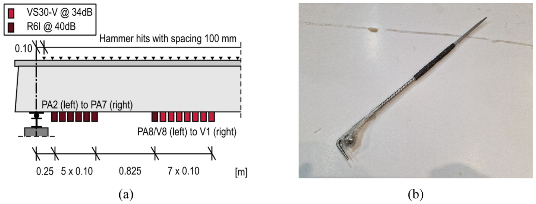
Measurement of the internal wave propagation properties using hammer hits on the top surface and sensors on the bottom surface: (a) sensor location and hammer hit location and (b) photo of the hammer, which had an angled tip and a steel ball.
Figure 6(b) shows the hammer that was used to hit the structural surface. The impact was introduced into the structure with the angled tip, validating the assumption of a point source. The steel ball attached to the rod served to increase the mass for the impact, thereby enhancing the energy emission of the signal. Compared to pencil lead break, hammer hits can generate source signals with larger amplitude, which can propagate for a longer distance before being attenuated to the noise level. Therefore, using hammer hits as sources, the ray path can be longer, resulting in a larger covering zone. In test 2, the ray path length reached 1 m using hammer hits as sources, while the ray path length was only around 0.5 m in test 1 using pencil lead breaks as sources.
However, hammer hits under the current setup were less controlled compared to pencil lead breaks. Human factors had more influence on the hammer hits regarding the strength of hitting. And the tip of the hammer may also generate noisier signals if the friction between the tip and the structural surface was not well controlled. This made the signals from hammer hits less reliable and less repeatable. Therefore, in the signal processing, the signals from the five hammer hits at the same location were averaged to reduce the effect of the large variation of the hammer hits.
Test 3: Measurement of possible damages in the bending zone and the shear zone
Region 1 and region 2 in Figure 4 are respectively the bending zone and the shear zone after the load is applied. Before loading, it is worth studying if any possible damage is already present.
To detect the possible existing damages in the two regions, UPV was performed right before the load testing when the AE sensors have been placed as planned in Figure 4. Each AE sensor was used as a transmitting transducer to emit a signal, and the other AE sensors received the signals. The emitted signal was a rectangular-shaped pulse of 5 μs duration.
UPV data analysis
UPV test estimates the wave velocity in a ray path using the wave travel distance and the wave travel time.

where c is the estimated wave velocity in the ray path from the source s to the receiver i, d s,i is the wave travel distance in that ray path, Ts,i is the arrival time at the receiver, and T s ,0 is the source time.
Test 3 can directly use Equation (2) to compute the wave velocity. However, the source time Ts,0 was unknown when using pencil lead break (test 1) and hammer hit (test 2) as the source. Therefore, we cannot directly calculate the wave velocity c for tests 1 and 2.
An alternative solution for the condition with an unknown source time is proposed. Assuming that two sensors i and j are receiving the signals from the same source s (which means the source time is the same) and the two ray paths share the same velocity c, we can use the signal arrival time difference and travel distance difference to calculate the wave velocity.
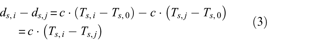
where d s,j and Ts,j are correspondingly the distance and the arrival time of the ray path from the source s to the receiver j.
In uncracked concrete, we can assume all the ray paths share the same velocity. Therefore, for a group of ray paths that originate from the same source, a linear relationship between the arrival time and the travel distance is expected. And the ratio between the travel distance difference and the arrival time difference is the estimated wave velocity.
In cracked concrete, some of the ray paths will be influenced by the crack, resulting in a delay of signal arrival times. The magnitude of the arrival time delay due to the crack is distinguishable compared to other factors, such as arrival time picking error. According to previous studies, a partially-closed crack will cause a delay of 20 µs, 27 while the arrival time picking error is less than 5 µs. 38 Without further verification, this magnitude of arrival time delay is used in this test. This method is not applicable if the crack affects all the ray paths, as it would cause a comparable delay across all the arrival times.
Figure 7 illustrates the UPV data analysis methods for the situation with an unknown source time. Figure 7(a) shows the two situations of UPV test 1 and 2, where the ray paths originating from the source s1 represent the case of UPV test 1, and the ray paths originating from the source s2 represent the case of UPV test 2. A vertical crack is assumed between sensors 5 and 6. The ray paths that are influenced by the crack are marked in red.
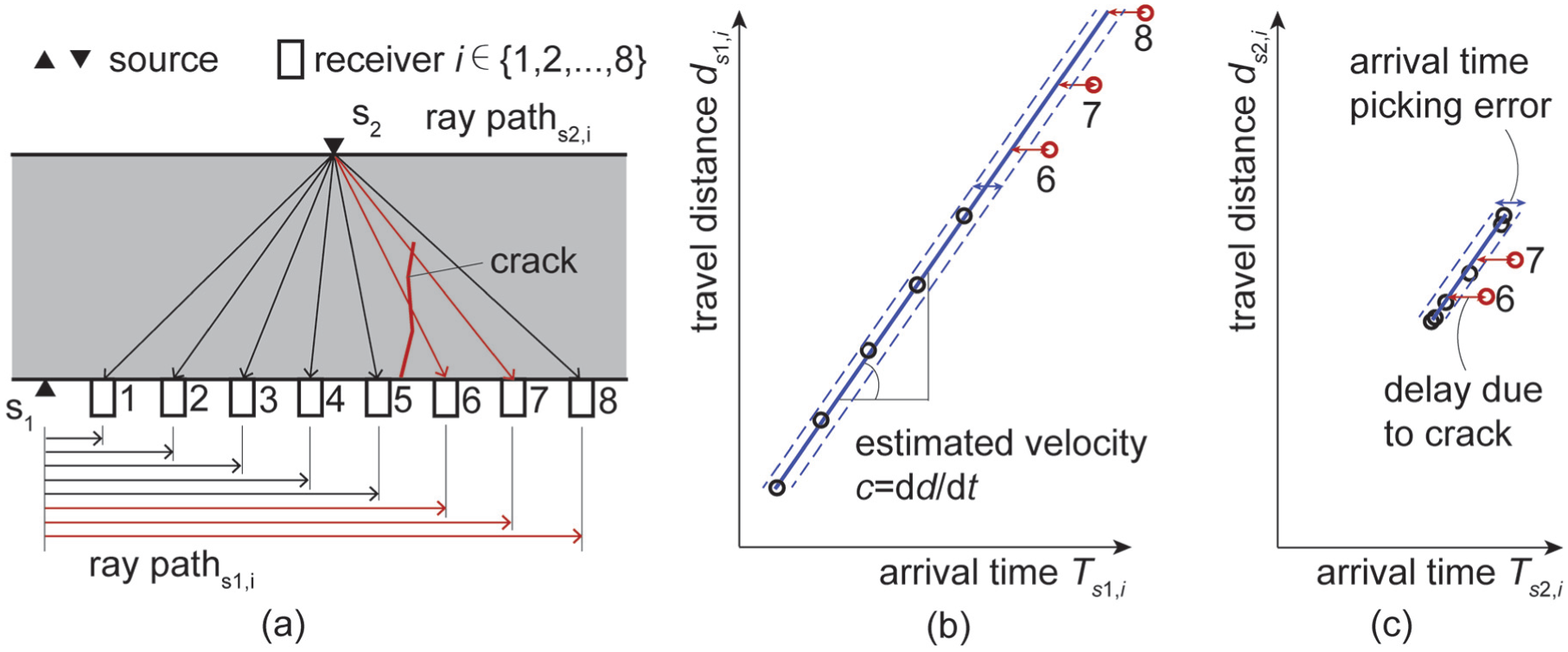
Illustration of crack identification using UPV with unknown source time: (a) the ray paths originated from the two sources, with the ones influenced by the crack marked in red, (b) the arrival time and the travel distance of the group of ray paths originated from the source s1, (c) the arrival time and the travel distance of the group of ray paths originated from the source s2. The linear relationship is marked by the solid blue line, and the arrival time picking error is shown by the dashed blue line. The arrival time picking error is marked by the red arrow. UPV: ultrasonic pulse velocity.
Figure 7(b) and (c) respectively show the estimation of wave velocity when the sources are s1 and s2. The solid blue line shows the linear relationship between the travel distance and the arrival time. The dashed blue line shows the margin of arrival time picking error. The ray paths that are influenced by the existing crack result in larger arrival time delay.
Acoustic emission
AE setup
Figure 4 shows the AE sensor layout. To ensure that an AE event can be captured by enough sensors for source localization (minimal three sensors for 2D localization in this case), the maximum sensor spacing was limited to 0.65 m.
To cover both the bending and the shear zone (regions 1 and 2 in Figure 4, respectively), two AE measurement systems were used because there was insufficient equipment within a single system to cover both regions simultaneously. In region 1, the Vallen sensors and data acquisition system were used,70,71 The applied Vallen sensors covered a frequency range from 25 to 85 kHz. In region 2, the PAC sensors and data acquisition system were used.72,73 The applied PAC sensors covered a frequency range from 40 to 100 kHz. The installation procedure for the AE sensors was the same as the one used for the UPV tests (Figure 5(b)).
Before applying the load, the noise level was recorded. To filter out the noise, a threshold of 65 and 45 dB was identified for the Vallen system and the PAC system, respectively. Only the signals with an amplitude higher than the threshold were recorded. The sampling rate to record the waveform was set to 1 MHz in the two systems.
AE data analysis methods
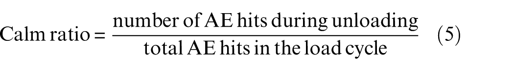
Cumulative AE hits with loading were computed. Based on the number of AE hits, load ratio, and calm ratio were counted in each load cycle, which is indicative of the structural damage level. 35 For uncracked concrete, the load ratio is usually not less than one, and the calm ratio is near zero. This paper uses the trend of reducing load ratio and increasing calm ratio to qualitatively indicate a more severe damage level. The computation of load ratio and calm ratio is as below.

Based on the hit arrival times and sensor locations, source localization was applied. 74 The measuring zone was discretized by a grid mesh with a grid point spacing of 5 mm. The distance between each grid point and the sensors was calculated. The best-fitted grid point should meet the requirement that the residual r between calculated and measured differential distance is the minimum.
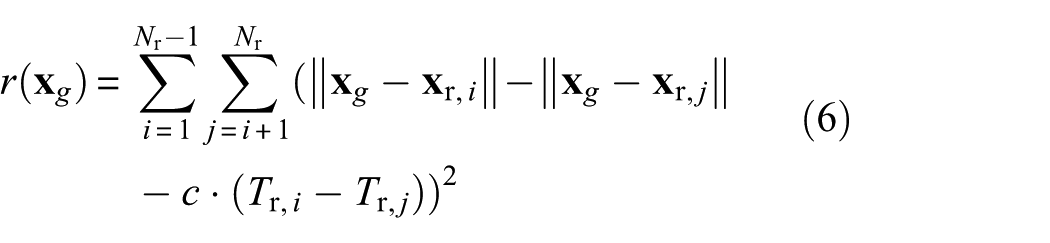
where
Based on the estimated source location, the probability density field of AE events (pdAE) was computed. 75 This pdAE includes the uncertainties in the localization and represents the probability/chance of AE events located at a certain position.
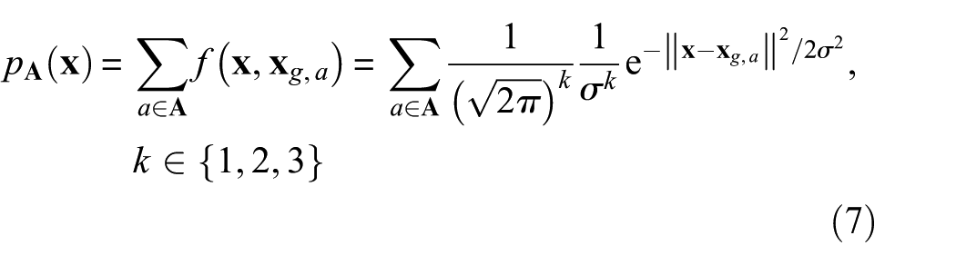
where
Distributed fiber optic sensors
DFOS measurement setup
A robust DFOS with a monolithic cross-section and a diameter of 3.0 mm was used. To improve the bonding properties, the outer surface of the DFOS was equipped with a braid so that mechanical interlocking with the adhesive was achieved. Experimental studies have shown that this specific DFOS type provides a stiff strain transfer between the concrete and the optical fiber, so that cracks can be detected at a very early stage (wcr < 0.01 mm). 23
As shown in Figure 4, the DFOS was installed on the tensile surface over a length of 9 m. To achieve optimal bonding conditions, the DFOS was glued in a 5 × 5 mm groove as shown in Figure 8. The installation process was as follows: after milling the groove and cleaning it with compressed air, the installation was carried out section-wise. First, a fast-curing two-component injection mortar was filled into the groove, then the DFOS was pressed into the adhesive matrix, and finally, the excess adhesive was removed with a spatula. This installation process ensured that the DFOS was fully embedded in the adhesive matrix.
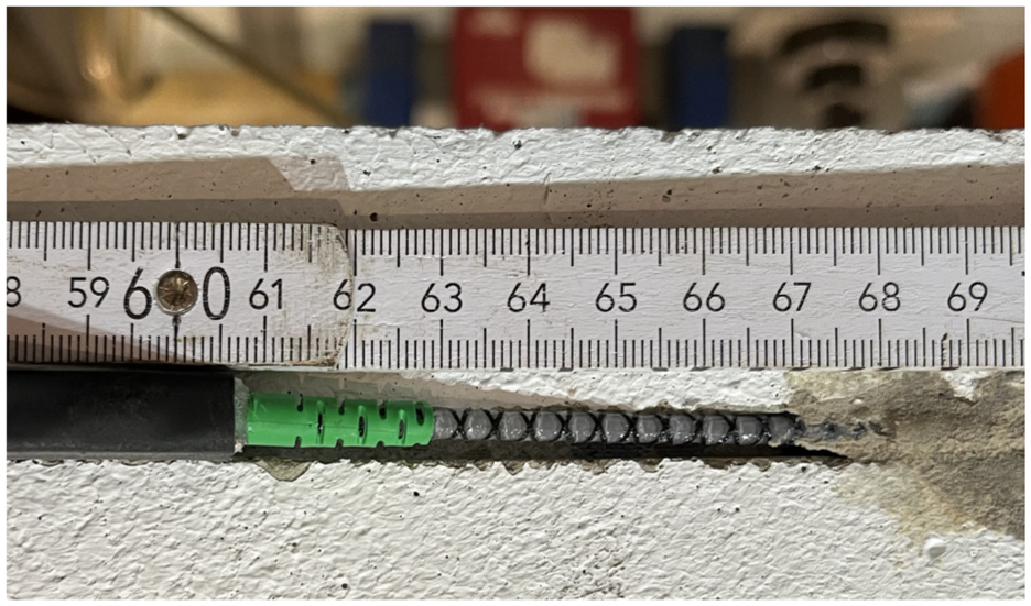
Installation of the DFOS in a 5 × 5 mm groove. DFOS: distributed fiber optic sensors.
The optical distributed sensor interrogator of the 6100 series, manufactured by Luna Inc. 77 , was used for the strain measurements. Since the DFOS was installed when the dead weight of the beam was activated, the strain changes due to the applied load were measured. During the load test, measurements were carried out at a frequency of 1 Hz and a gage pitch (spatial resolution) of 1.3 mm. The manufacturer specifies a measuring range of ±12,000 μm/m, a resolution of 1 μm/m, and an accuracy of ±16 μm/m for the selected measurement settings. 78
DFOS data analysis
The evaluation of DFOS data was carried out using the free open-source software framework fosanalysis. 79 Fosanalysis offers a streamlined workflow from parsing the raw data, via preprocessing, up to automated crack detection and crack width calculation.53,58
Strain profiles were retrieved by taking the temporal median over a few readings to reduce noise and disturbances. Then, the strain profile is smoothed along the space-axis using a sliding median with a window radius of three entries, which eliminates the remaining SRAs. This approach was appropriate for the data set at hand and resulted in a reliable crack evaluation. Another option would be to employ dedicated SRA detection algorithms. 58 Dropouts were reconstructed by interpolating the missing values using local Akima-splines. 80
The positions of cracks in the final stabilized crack pattern (called reference positions) were extracted from the last loading step L5 using the workflow implemented in FOSANAYSIS. 53 Crack detection employed peak finding with a prominence threshold of 100 μm/m and a total height threshold of 1000 μm/m. The transfer lengths of the cracks were limited by the local strain minima between two cracks. Finally, crack widths were calculated by integrating the strain profile over the transfer lengths.
Results
Load-deflection behavior
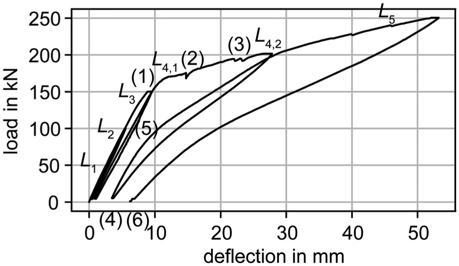
Figure 9 shows the load-deflection behavior during the load testing. The transition to the cracked state is characterized by a significant stiffness reduction at a load level of about 170 kN, shown in Figure 9 (1). This load is close to the calculated cracking force of 183 kN in “Determination of relevant load situations” section. Therefore, significant pre-damage of the tendons due to SCC is not expected. Deviations between the observed and calculated cracking force may result from variations in concrete tensile strength.
The load–deflection behavior.
The loading was force-controlled and temporarily displacement-controlled in L4.1. Hence, the force reduction in plateau L4,1 due to creep is found in Figure 9 (2). The two drops in the load-deflection curve between 190 and 200 kN, as shown by Figure 9 (3), correspond to the opening of two cracks. After reaching the load plateau at 200 kN, the girder was unloaded, whereby inelastic deformations became visible, as shown by Figure 9 (4). The repeated loading and unloading reveal the typical hysteresis loops of concrete, where the specimen behaved stiffer in the loading compared to the unloading.81,82
In the loading up to L5, after reaching the decompression force at approximately 90 kN, a stiffness reduction was observed compared to the previous loading phases, as shown by Figure 9 (5). This indicates that the girder was damaged in the previous load cycle L4 (200 kN). Except for a small amount of tension stiffening between the cracks, the concrete in the tension zone no longer contributed to the load transfer, leading to stiffness reduction at the decompression state. Since no such stiffness reduction was observed in the loading phase of the previous load cycles, we can state that the girder has never been loaded greater than 200 kN in its service life. After unloading from L5, a large inelastic deformation of approximately 7.5 mm remained, as shown by Figure 9 (6).
Before loading: Detection of the existing cracks
UPV test 1 result
UPV test 1 measured the wave velocity on the structural surface, where no open crack was observed. Figure 10(a) shows the received signals when a pencil lead break was performed at 0.05 m to the PAC sensor P7 in location 1 (the location is marked in Figure 5(a)). The arrival times were picked using the Akaike Information Criterion method 83 (Figure 10(b)). The wave velocity was estimated as outlined in “UPV data analysis” section.
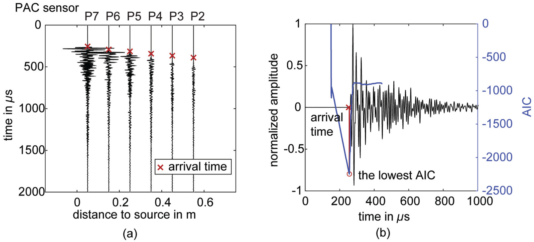
(a) Received signals from pencil lead break at 0.05 m to the PAC sensor P7 in location 1 (the location can be found in Figure 5(a)), with the arrival times marked by the red crosses, and (b) an example of arrival time picking using Akaike Information Criterion in the normalized signal received by PAC sensor P7.
Figure 11(a), (b), and (c), respectively, show the measured arrival times and travel distances in locations 1, 2, and 3 (the locations are marked in Figure 5(a)). The solid blue line shows the estimated linear relationship between the wave travel distance and the wave arrival time, and the dashed blue line shows a margin of ±5 µs due to the expected arrival time picking error. The dashed red line shows the expected arrival time difference of ±20 µs if a partially closed crack is present in the ray path from the source to the sensor.
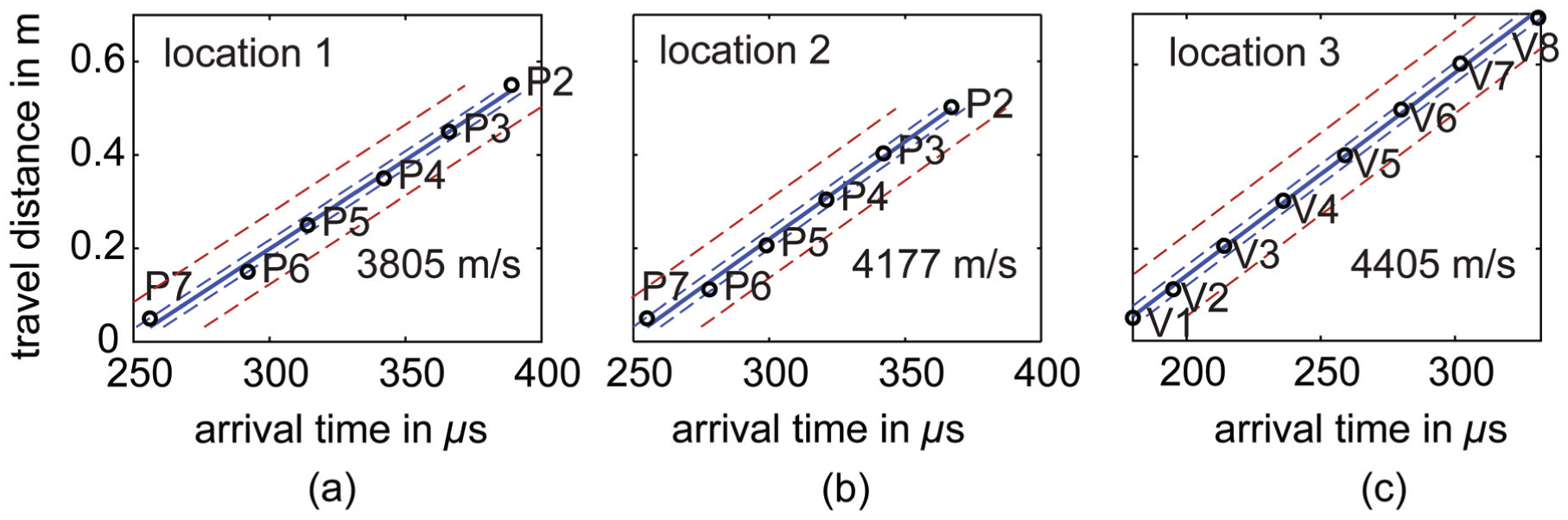
Estimation of wave velocities in (a) location 1, (b) location 2, and (c) location 3. The locations can be found in Figure 5(a). The solid blue line shows the estimated linear relationship between the travel distance and the arrival time, the dashed blue line shows the expected arrival time picking error, and the dashed red line shows the expected influence of a partially-closed crack.
In every location, the variation of the arrival times was minimal, within the expected error due to arrival time picking. Therefore, no crack is expected in these three locations at the time of UPV test 1.
The estimated wave velocity in the three locations 1, 2, and 3 were, respectively, 3805, 4177, and 4405 m/s. A lower wave velocity was found in location 1, which was on the top surface. This might be due to the different concrete material in the cast-in situ layer, or stress state. Under self-weight and prestressing force, the top part of the girder was under tension and the bottom part was under compression. The wave velocity of concrete under tension can be lower than that of concrete under compression. 84 Moreover, the velocities in locations 2 and 3, which were both on the bottom surface, also differed. This might be due to the spatial variation of the concrete material properties. Such variation of velocity in uncracked concrete has been observed in other experiments. 85
UPV test 2 result
UPV test 2 measured the wave velocity across the whole height of the girder and in the center plane of the cross section in the width direction. Both the PAC and the Vallen systems were applied to capture the signals from the hammer hits. However, it is found that the signals received by the PAC system exhibited a lower signal-to-noise ratio, which might be related to the system setup. Without additional processing of the weaker PAC signals, this study primarily utilized signals recorded by the Vallen system. Additionally, due to wave attenuation, only ray paths shorter than 1 m were considered. After applying these two filtering criteria, 80 ray paths were selected for analysis. Figure 12a shows the ray paths from the source to the receivers.
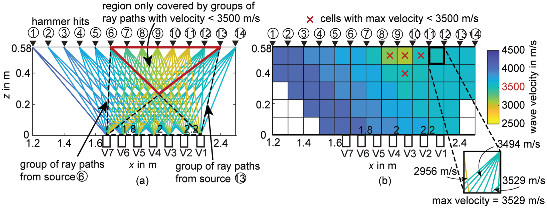
(a) A total of 14 groups of ray paths, each group originating from the same source. The regions covered by ray paths from hammer hits 6 and 13 are enclosed by dashed black lines as examples. The color of the ray paths indicates the estimated wave velocity. The region enclosed by a red triangle was only covered by ray paths with velocity lower than 3500 m/s, and the other region was covered by at least a group of ray paths with wave velocity higher than 3500 m/s, (b) a visualization displaying the maximum velocity from all ray paths passing through a specific cell. The determination of the maximum velocity in the cell between hammer hits 11 and 12 is shown as an example. The cells with maximum velocity lower than 3500 m/s are marked with a red cross.
A total of 14 groups of ray paths are identified: each group includes the ray paths originating from the same source. The region covered by the group of ray paths from the hammer hits 6 and 13 are shown as examples by the dashed black lines in Figure 12(a).
Following the method outlined in “UPV data analysis” section, Figure 13 shows the estimation of the wave velocity in each group of ray paths originating from the same source. In each group, no ray path had arrival time delay reaching the expected value due to a crack (indicated by the dashed red lines). This means for a group of ray paths originating from the same source, no major crack is expected within the region covered by that group of ray paths. This did not apply if the crack in the region influenced all the ray paths as stated in “UPV data analysis” section.
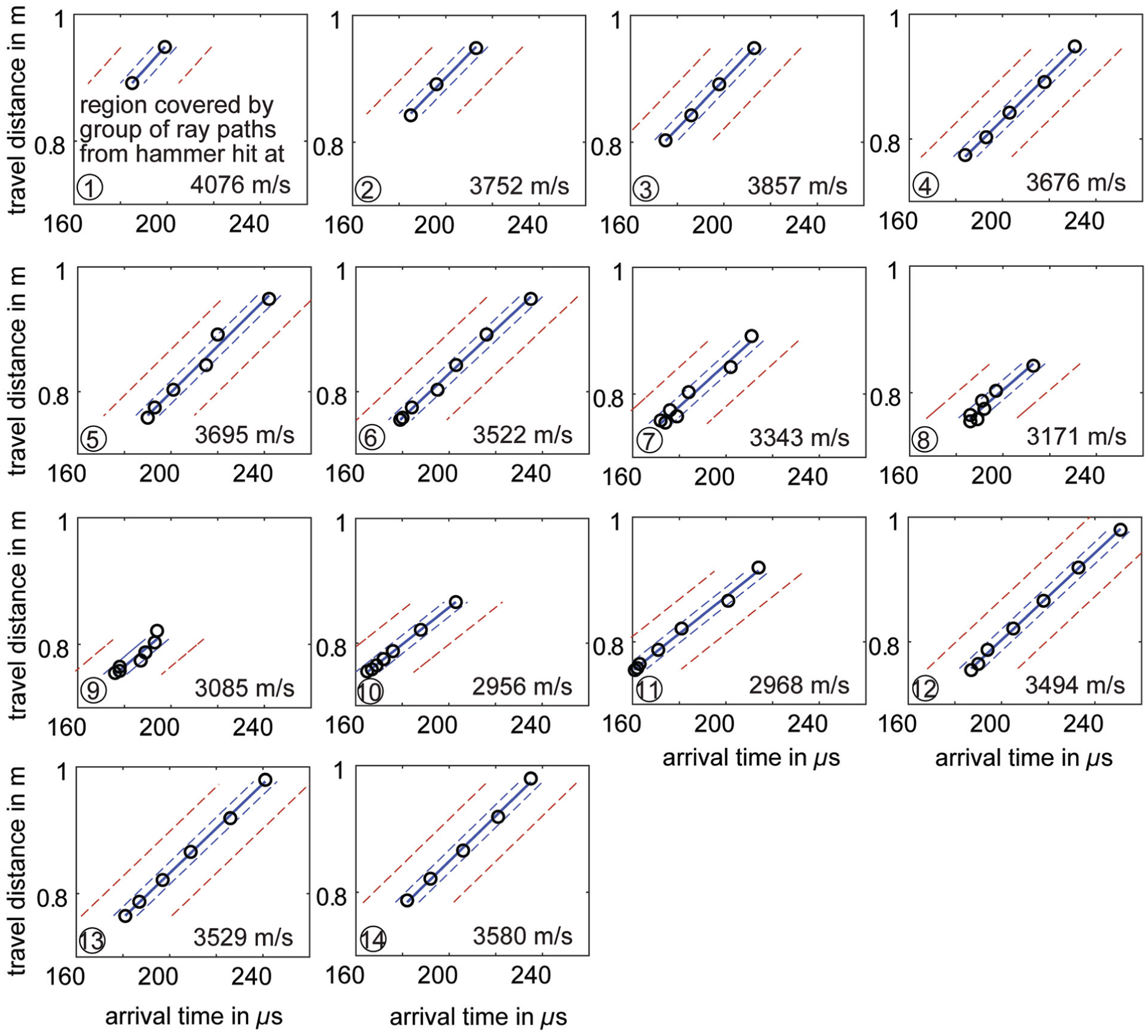
Estimation of wave velocity in each group of ray paths originating from the same hammer hit source. The locations of the hammer hits can be found in Figure 12. The solid blue line shows the estimated linear relationship between the travel distance and the arrival time, the dashed blue line shows the expected arrival time picking error, and the dashed red line shows the expected influence of a partially-closed crack.
The estimated wave velocity in different groups varied from 2956 to 4076 m/s. By plotting the spatial distribution of the wave velocity (Figure 12(a)), the low wave velocity (<3500 m/s) was found in the ray paths which were originated from the sources 7 to 12. As a result, a region near the top surface was only passed by the ray paths with low wave velocity (shown by the red triangle in Figure 12(a)). The other region was covered by at least one group of ray paths with wave velocity larger than 3500 m/s.
Figure 12(b) offers an alternative visualization of regions with lower wave velocity. The measurement zone is divided into 0.1 × 0.12 m cells, displaying the highest velocity recorded among all ray paths passing through each cell. As an example, the determination of the maximum velocity in the cell between hammer hits 11 and 12 is illustrated. Cells with maximum velocities below 3500 m/s are marked with a red cross, effectively highlighting reduced wave velocities near the top surface, particularly between hammer hits 8–11. However, this visualization does not represent the actual wave velocity within each cell. Additionally, the choice of cell size and the statistical metric (such as using maximum velocity) have not been validated.
There are two reasons for using 3500 m/s as the threshold. The first reason is that empirically the velocity in uncracked concrete is above 3500 m/s. 63 Besides, it was found in the literature, that the variation of velocity in uncracked concrete was around 5% (the standard deviation divided by the mean). 85 Supposing that the mean velocity was 3805 m/s as measured in UPV test 1, the standard deviation would be around 190 m/s. The 95% of the values would be within 2 standard deviations of the mean, which was between 3425 m/s and 4185 m/s. Therefore, the value of 3500 m/s, which was slightly above the lower bound 3425 m/s, would be a reasonable criterion to evaluate the concrete quality near the top surface.
Therefore, the wave velocity below 3500 m/s near the top surface may indicate localized material degradation, such as poor concrete quality or delamination between the cast-in situ layer and the precast girder. If delamination were the reason, it would need to extend across all ray paths originating from sources 7–12 to uniformly affect the measurements. Otherwise, the discrepancy in arrival times between affected and unaffected ray paths would be significant enough to reach the dashed red lines in Figure 13 which was not observed.
UPV test 3 result
UPV test 3 measured the wave velocity in a larger area covering the bending zone and the shear zone (region 1 and region 2 in Figure 4). Figure 14(a) exemplifies the received signals at each sensor when PAC sensor P3 was sending signals working as the source. Since the source time was recorded by the source sensor, the wave velocity in a ray path was calculated using Equation (2) directly. Due to signal attenuation, only the ray paths shorter than 1 m were considered.
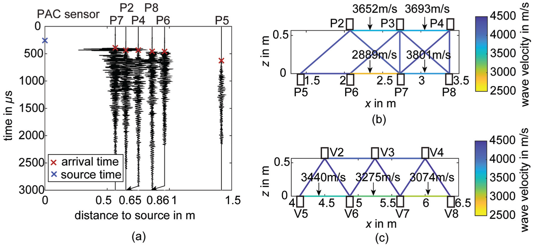
Estimation of the wave velocity right before the load test: (a) signals received by PAC sensors when sensor P3 was the source, with the source and the arrival times marked, (b) spatial distribution of the wave velocity in the shear zone, and (c) spatial distribution of the wave velocity in the bending zone.
Figure 14b shows the wave velocity distribution in the shear zone right before the load test. On the top surface, the lowest velocity was found in the ray path P2–P3, which was 3652 m/s. The velocity was higher than 3500 m/s and was close to the reference velocity of uncracked concrete on the top surface, which was 3805 m/s. On the bottom surface, the lowest velocity was found in the ray path P6–P7, which was 2889 m/s. This velocity was below 3500 m/s and was much lower than the reference velocity for the uncracked concrete on the bottom surface, which was 4177 m/s. This much lower velocity compared to the reference could indicate possible damage near surface in the ray path P6–P7 before the load test.
Figure 14c shows the wave velocity in the bending zone right before the load test. Most ray paths had wave velocity close to the reference velocity, except for ray paths V5–V6, V6–V7, and V7–V8 on the bottom surface. The velocities in these ray paths were respectively 3440, 3275, and 3074 m/s, indicating possible damage near surface before the load test.
The possible damages on these ray paths on the bottom surface are expected to be limited in height, since the adjacent internal ray paths did not exhibit reduced wave velocities. This damage near the bottom surface could be attributed to early-age shrinkage or to the relatively low traffic loads experienced during the service life.
At low-load cycle: Verifying the existence of cracks
DFOS result at low-load cycle
DFOS served as the primary technique for verifying the presence of existing cracks. Figure 15 shows the strain distribution along the beam at load level L1 = 50 kN. Although the load was below the decompression force and the girder was under compression, the DFOS strain profile revealed minor strain peaks, indicating localized stress variations.
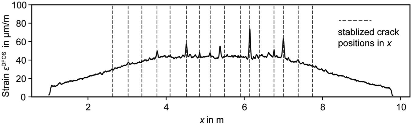
Strain profile at L1 with some minor strain peaks (crack locations in the stabilized crack pattern are indicated by dashed vertical lines).
The locations of these strain peaks further reinforce the findings of UPV test 3, confirming the presence of cracks on the bottom surface near mid-span. Notably, the DFOS-detected crack locations were far more precise than those identified by UPV, aligning exactly with the stabilized crack pattern observed at L5 (indicated by dashed vertical lines in Figure 15).
Crucially, the detection of these strain peaks at low-load level L1, when the section was still in compression, highlights a key advantage of DFOS—its ability to identify existing cracks in prestressed concrete structures before tensile forces are present at crack locations.
AE result at low-load cycle
Figure 16(a) and (b) show the number of AE hits received by the PAC sensors (in total, seven sensors in the bending) and Vallen sensors (in total, eight sensors in the shear zone) respectively. Notably, very few AE hits were detected during unloading in the initial load cycle (L1), suggesting minimal friction between the crack surfaces when unloading from 50 kN.
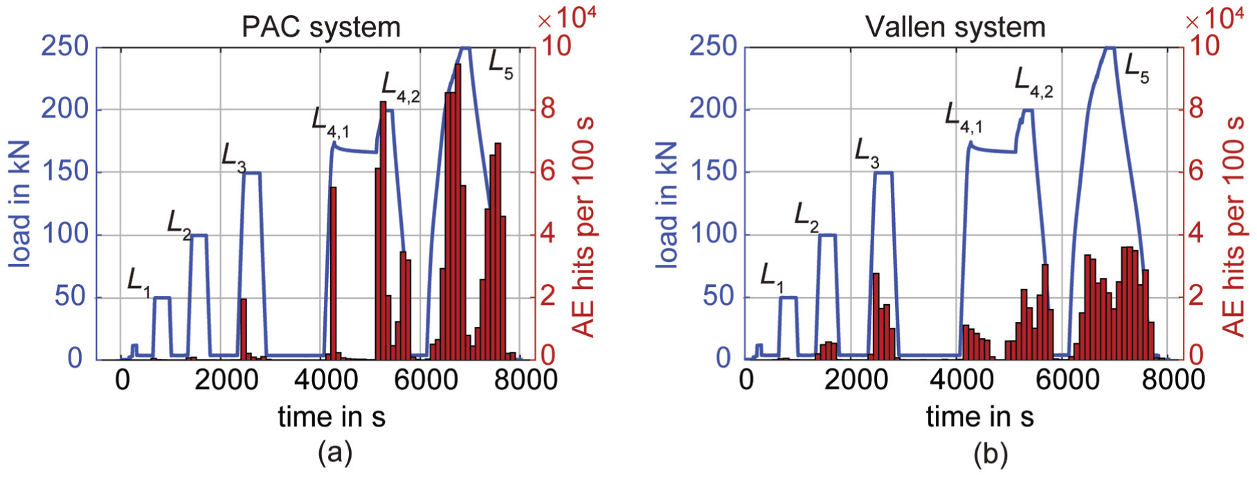
Number of AE hits per 100 s in the loading history: (a) recorded by all PAC sensors and (b) recorded by all Vallen sensors. AE: acoustic emission.
In contrast, during later load cycles (L4 and L5), a significant amount of AE hits was observed during unloading, even from the same 50 kN load level. In those phases, the existing cracks were also not expected to be opened, but the re-compression during unloading generated significantly more AE hits than in L1. This might be because some cracks in L4 and L5 were newly formed, and the crack surfaces were not smoothened, resulting in more friction during re-compression.
At higher-load cycles: Monitoring the crack formation and development
AE result at higher-load cycles
AE hit analysis
In each load cycle, the onset of cracking was identified when the cumulative number of AE hits exceeded 200 from the previously unloaded state. Figure 17 exemplifies the determination of the onset of cracking in L3 in sensor P6. When a threshold of 200 AE hits was applied, the onset load was around 135 kN.
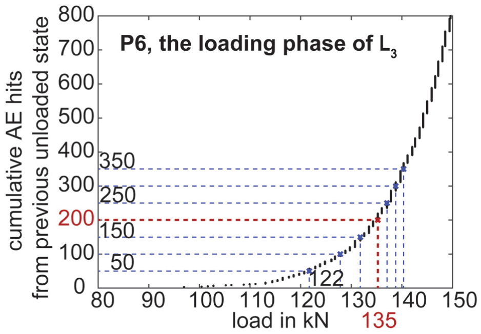
Influence of threshold on determination of AE hit onset load for sensor P6. AE: acoustic emission.
Although the threshold value of 200 was chosen arbitrarily, we analyze its impact by varying it by ±75% (i.e., from 50 to 350). This change results in a deviation of approximately ±13 kN from the baseline value of around 130 kN (Figure 17 and Table 2). Moreover, the influence of the threshold decreases as the threshold value increases, indicating a diminishing sensitivity at higher levels.
Determination of AE hits onset using different thresholds on sensors P6, P8, V5, and V6.
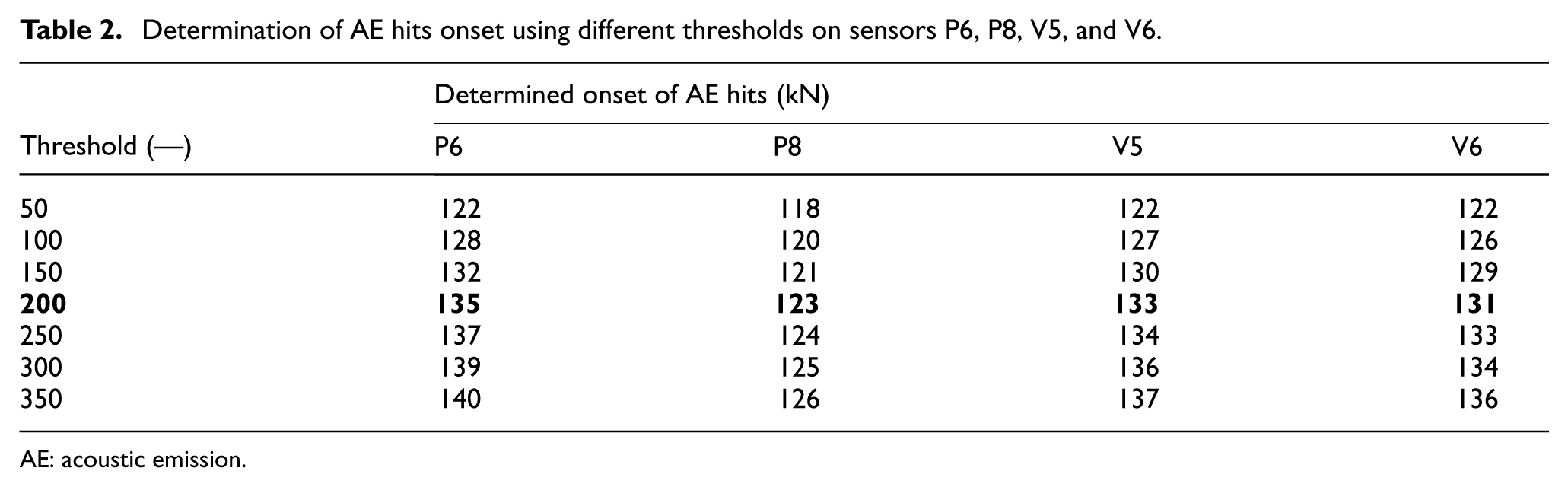
AE: acoustic emission.
Figure 18 illustrates the cumulative AE hits recorded by four sensors positioned on the bottom surface: P8 and P6 from the PAC system, and V5 and V6 from the Vallen system. In the PAC system, sensor P8 detected crack opening at approximately 123 kN, about 10 kN earlier than sensor P6. This earlier cracking near P8 aligns with expectations, as the estimated bending moment in that region was higher than near P6.
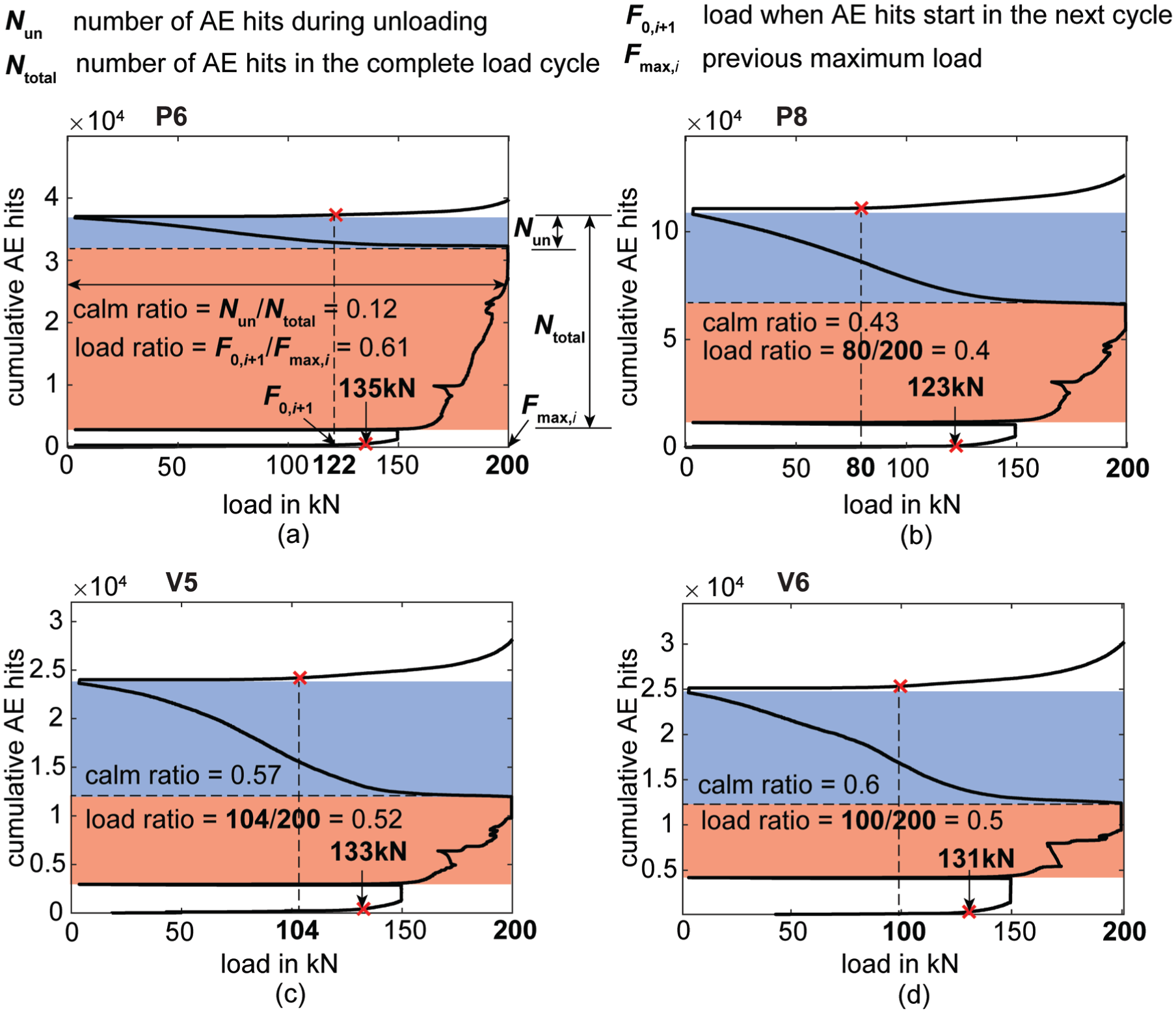
Increase of cumulative AE hits with load recorded by sensors: (a) P6, (b) P8, (c) V5, and (d) V6. The onset of AE hits is marked using red crosses. The calculation of calm ratio and load ratio based on hits is exemplified using load cycle L4. The total number of hits in the load cycle is noted as Ntotal, the number of hits in the unloading phase is noted as Nun, the load at the onset of AE hits in the next load cycle is noted as F0, i +1, and the previous maximum load is noted as Fmax, i . AE: acoustic emission.
In the Vallen system, sensors V5 and V6 detected crack formation at nearly the same load levels, 133 and 131 kN, respectively. This was also anticipated, given that both sensors were positioned in a region of constant bending moment. However, a direct comparison of the crack onset detected by the two systems is not feasible due to differences in noise levels, which influence the number of recorded AE hits.
Calm ratio and load ratio analysis
Load ratio and calm ratio were used to qualitatively evaluate the damage level. The calculation of the load ratio and calm ratio is exemplified at the selected sensors P6, P8, V5, and V6 at load cycle L4 (shown in Figure 18). Among these sensors, P6 showed a lower calm ratio and higher load ratio, indicating a lower damage level in the area around sensor P6. This meets the expectation since the sensor P6 was farther from the loading plate where the bending moment was smaller.
Figure 19 shows the load ratio and calm ratio at all the Vallen sensors at different load cycles. The results show that the bending zone of the girder was not seriously damaged before 100 kN (Figure 19(a) and (b)). An exception was the sensor V3 on the top surface which showed a load ratio less than 1 at the load cycle L2 = 100 kN. This might be due to local damage near V3, such as friction between the in situ concrete layer and the precast concrete girder.
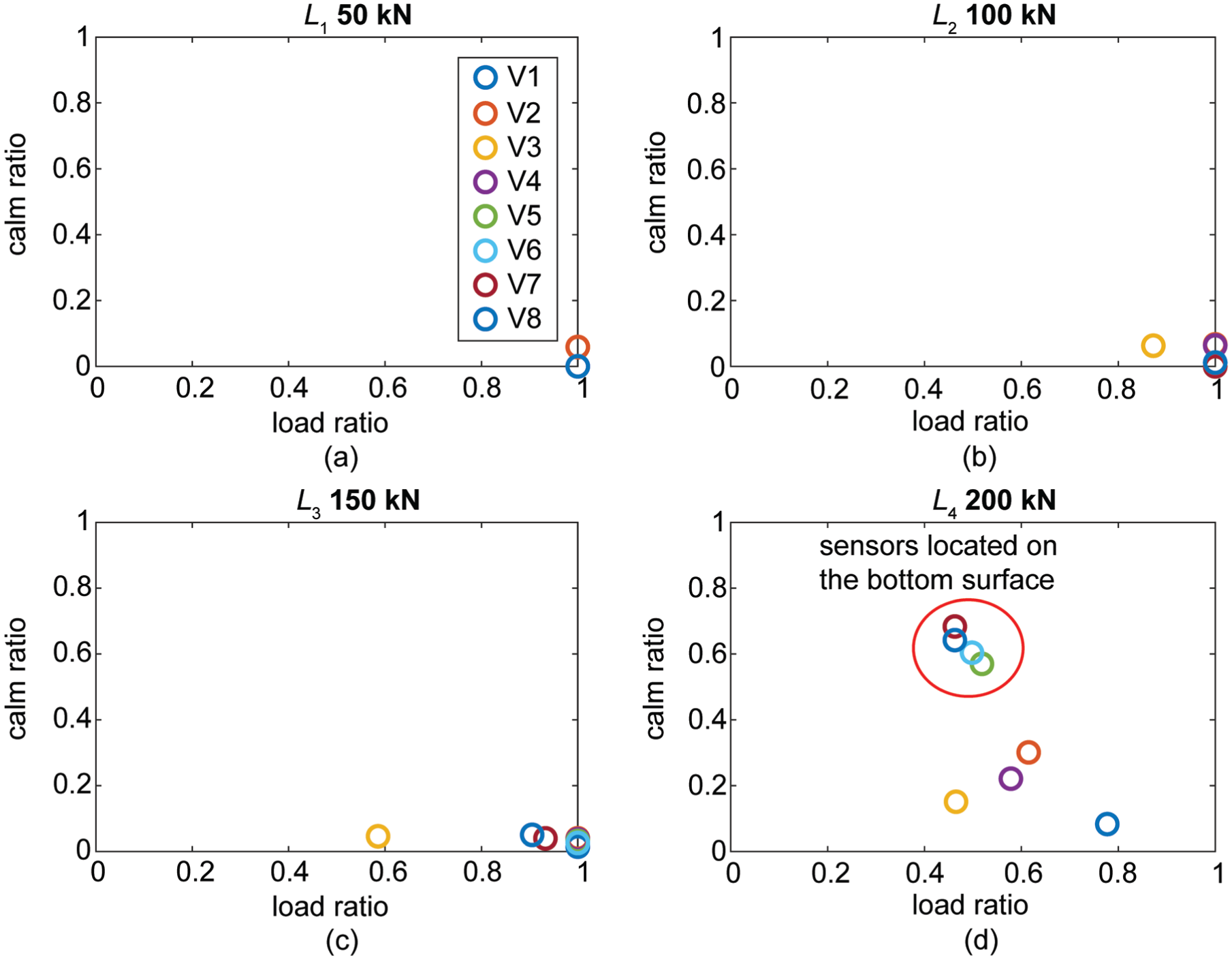
Load ratio and calm ratio at Vallen sensors at different load cycles: (a) L1, (b) L2, (c) L3, and (d) L4.
At load cycle L3 = 150 kN (Figure 19(c)), sensors V7 and V8 on the bottom surface showed lower load ratios, indicating possible local damage. At load cycle L4 = 200 kN (Figure 19(d)), more sensors indicated possible local damage around them, and the bottom surface was shown to be more damaged.
Figure 20 shows the load ratio and calm ratio at all the PAC sensors at different load cycles. The results show that the shear zone of the girder was not seriously damaged before 100 kN (Figure 20(a) and (b)). At load cycle L3 = 150 kN (Figure 20(c)), the sensor P8 started to show lower load ratio, indicating possible damage. This meets with the expectation that the cross section near P8 had larger bending moment than the cross sections near other sensors in the shear zone. At load cycle L4 = 200 kN (Figure 20(d)), more sensors indicated damage around them. The region with larger bending moments (closer to the loading plate and on the bottom) was shown to be more damaged.
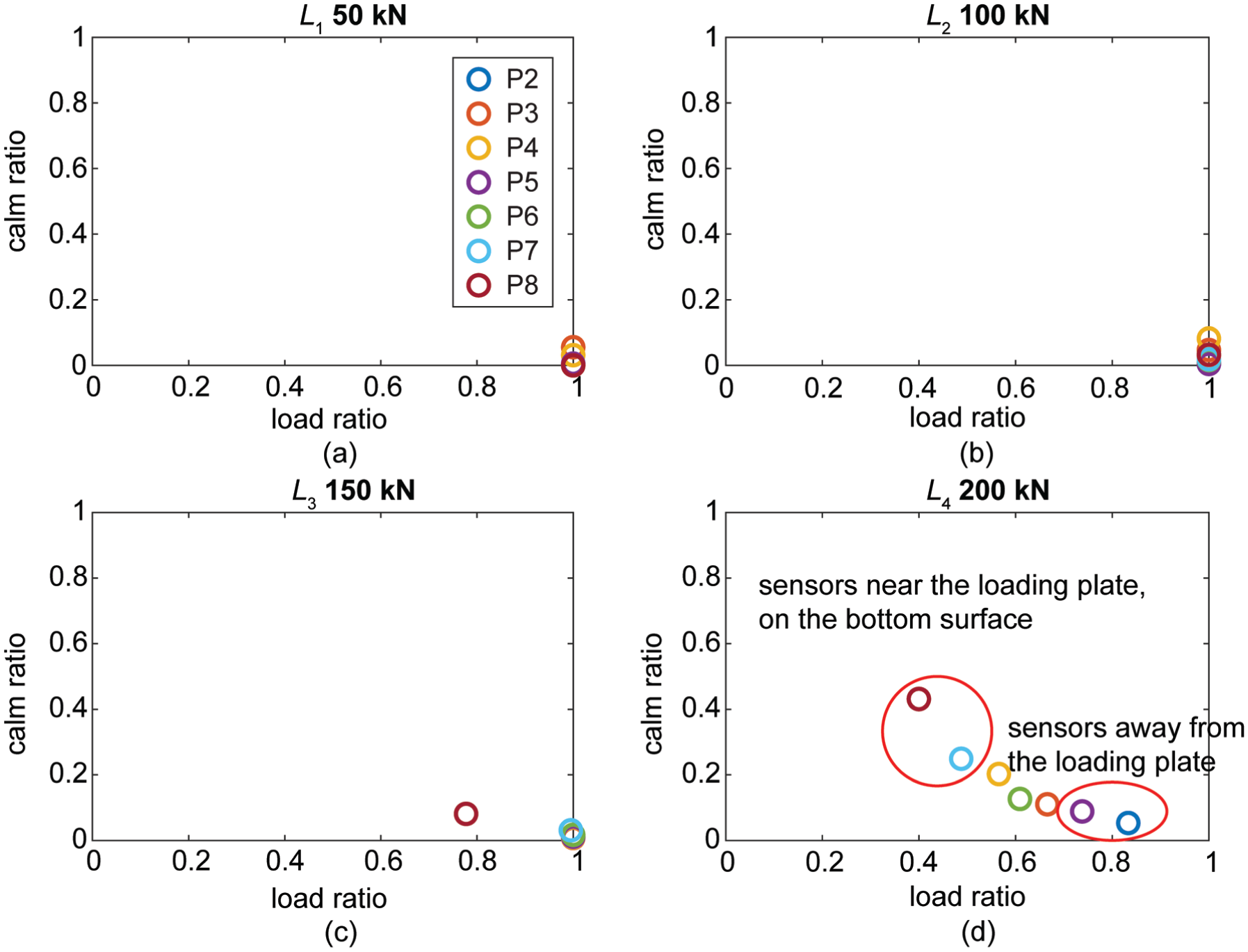
Load ratio and calm ratio at PAC sensors at different load cycles: (a) L1, (b) L2, (c) L3, and (d) L4.
Source localization
Figure 21 shows the localization results at different load levels in the bending zone including the estimated source location and the pdAE field. Aligned with the results of hit analysis, calm ratio and load ratio analysis, the source localization results show that new cracks opened first in the bending zone in the load cycle L3 between 100 to 150 kN.
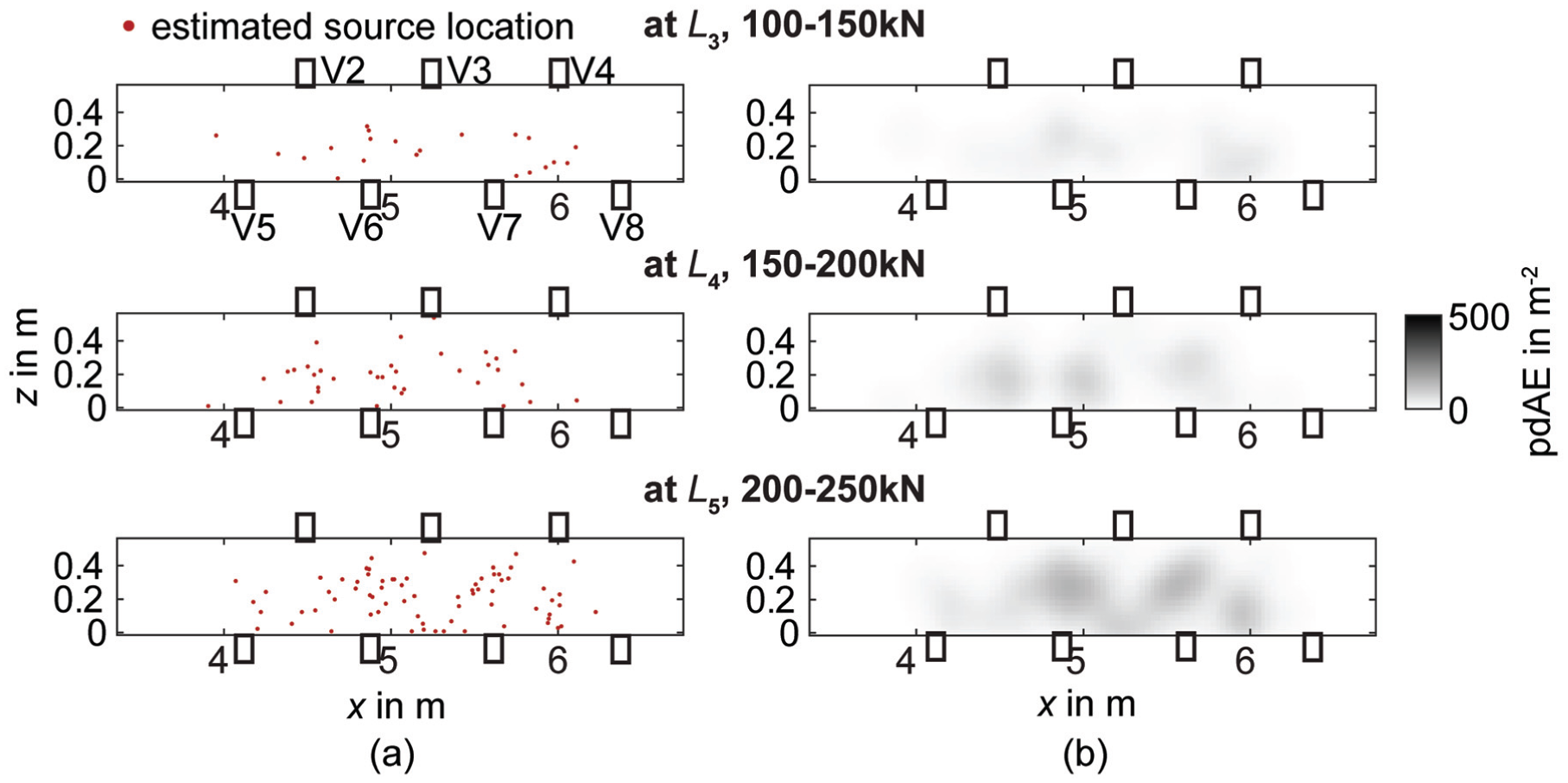
Source localization results using signals recorded by the Vallen sensors in the bending zone when reaching load levels of L3 (150 kN), L4 (200 kN), and L5 (250 kN): (a) the estimated source localization and (b) pdAE. pdAE: probability density field of AE event.
Figure 22 shows the localization results at different load levels in the shear zone. At load step L4 (150–200 kN), besides flexural cracks, which started from the bottom of the girder, we first observed localized AE events in the web, at around 3 m to the support (0.75 m to the loading plate). This might be related to the formation of the crack in the web where the cross-section width is small. 86 This crack later developed into the bottom of the girder when approaching L5 (250 kN). However, this interpretation cannot be directly verified since the region in the internal web where the crack was suspected to initiate was not measured by other sensors. Moreover, the AE source localization was also not sufficiently accurate. This could be validated by destructive testing such as sawing or cutting the girder at the estimated crack location.
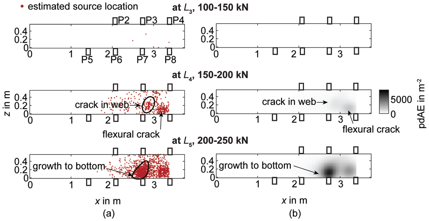
Source localization results using signals recorded by the PAC sensors in the shear zone when reaching load levels of L3 (150 kN), L4 (200 kN), and L5 (250 kN): (a) the estimated source localization and (b) pdAE. pdAE: probability density field of AE event.
DFOS result at higher load cycles
Strain profiles over the test
Figure 23 shows the strain profiles during the loading plateaus of L1 through L5. The locations and the crack width of the stabilized cracks in L5 are marked in red dots. Crack widths were calculated using the strain integration approach using local minima as integration limits and taking tension stiffening into account. 53 Because the temperature in the lab can be assumed constant, dedicated temperature compensation was omitted. Comparing the strain profiles reveals progressive cracking of the beam. Based on the first appearance of the peaks, it can be deducted in which load cycle a crack developed. For example, the crack at 5.9 m formed in L5, and the crack at 5.13 m formed in L3.
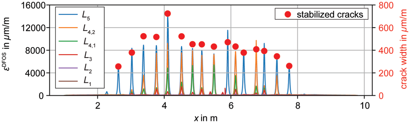
Strain profiles for all load levels L1 through L5 and the stabilized cracks detected and calculated at L5.
Differentiation between new and existing cracks
Figure 24 exemplifies the differentiation between new and existing cracks using the strain profiles captured during L3 = 150 kN between x = 4.4–5.2 m. The strain profiles were captured at four consecutive time stamps with an increment of 15 s from a load level of 111.1 kN, which was higher than the previous maximum load (L2 = 100 kN). The first crack—located at 4.52 m—probably existed before load testing (according to Figure 15). A strain peak was already found at dt = 0 s. The second crack—located at 5.13 m—formed at around dt = 30 s at load level of 140.3 kN. Based on the strain differences between two consecutive time points (i.e., differential strain profiles), it is possible to calculate crack width changes. 54
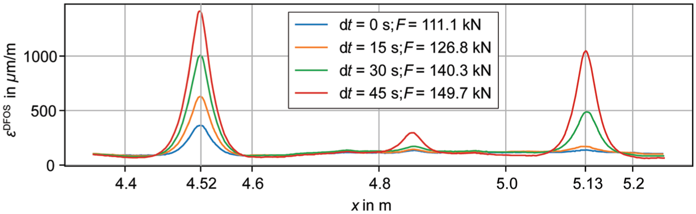
Selected strain profiles from DFOS measurements during L3. DFOS: distributed fiber optic sensors.
Figure 25 shows the respective load–strain curves at the cross sections of the two selected cracks during L1, L2, and L3. Four stages in a loading cycle can be observed: (i) linear-elastic behavior with high cross-sectional stiffness, (ii) crack growth leading to stiffness reduction, (iii) reduced stiffness during unloading, and (iv) residual strain when unloaded.
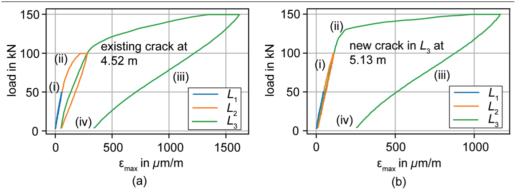
Load–strain behavior of: (a) an existing crack at 4.52 m and (b) a crack newly developed in L3 at 5.13 m.
The load–strain curve for the cross section at 4.52 m with the existing crack, deviates from the linear-elastic path already in L2 at around 60 kN to 80 kN (Figure 25(b) (ii)). Note that this disproportional strain increase starts below the calculated decompression force of 84 kN. The existing crack started to grow considerably at about 110 kN in L3. Compared to that, the load-strain curve bends sharply when a new crack forms (Figure 25(a) (ii)).
On the unloading path, both cracked cross sections behave similarly in stage (iii) and stage (iv). A possible indicator of new and existing cracks is the strain rate at stage (ii). The derivation of the load–strain curve is considerably sharper when a new crack form compared to the growth of existing cracks.
Strain development at the reference locations
Figure 26 shows the strain development at the reference crack locations in the constant bending moment zone. The strain development at most crack positions qualitatively corresponds to the global load–displacement curve (Figure 9(b)).
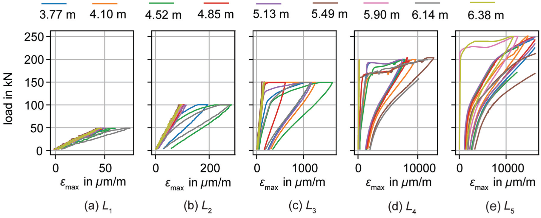
Force-strain development at reference locations through loading cycles (a) L1 to (e) L5.
At the first load cycle L1 (Figure 26(a)), most reference positions were still uncracked, therefore the load–strain curves were linear. In L2 (Figure 26(b)), three strain peaks belonging to the existing cracks increased over-proportionally which were at the locations of 3.77, 4.52, and 6.14 m.
In L3 (Figure 26(c)), the maximum strains of the three existing cracks increased over-proportionally, indicating the growth of the existing cracks. When the girder was loaded with 130 kN, a new crack developed at locations of 5.13 m. This aligns with the cracking load levels determined by AE hits in “AE hit analysis” section where sensors V5 and V6 recorded it around 130 kN which were installed in the constant bending moment zone. Hence, it can be deduced that the beam was never subject to a load equivalent to F = 130 kN. Afterwards, at around 150 kN two more new cracks developed at locations of 4.10 and 4.85 m.
In L4 (Figure 26(d)), the girder reached an almost stabilized crack pattern with one new crack formed at the location of 5.49 m. In L5 (Figure 26(e)), two more cracks formed at the locations of 5.90 and 6.38 m.
Possible link between AE hit and DFOS strain
The previous analysis shows that new crack opening caused an increase in both AE hits and accelerated strain increase in the crack locations. Hence, it is assumed that the AE hits and the DFOS strain measurements can be related. To test this hypothesis, a new parameter is computed, which is the time-dependent DFOS strain rate. This parameter measures the strain development of all cracks with respect to time.
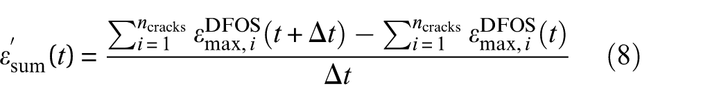
where
Correspondingly, the time-dependent AE hit rate is calculated based on the same cracks over time.
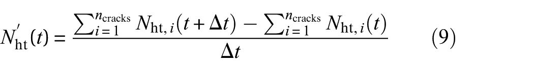
where
Figure 27 compares both parameters
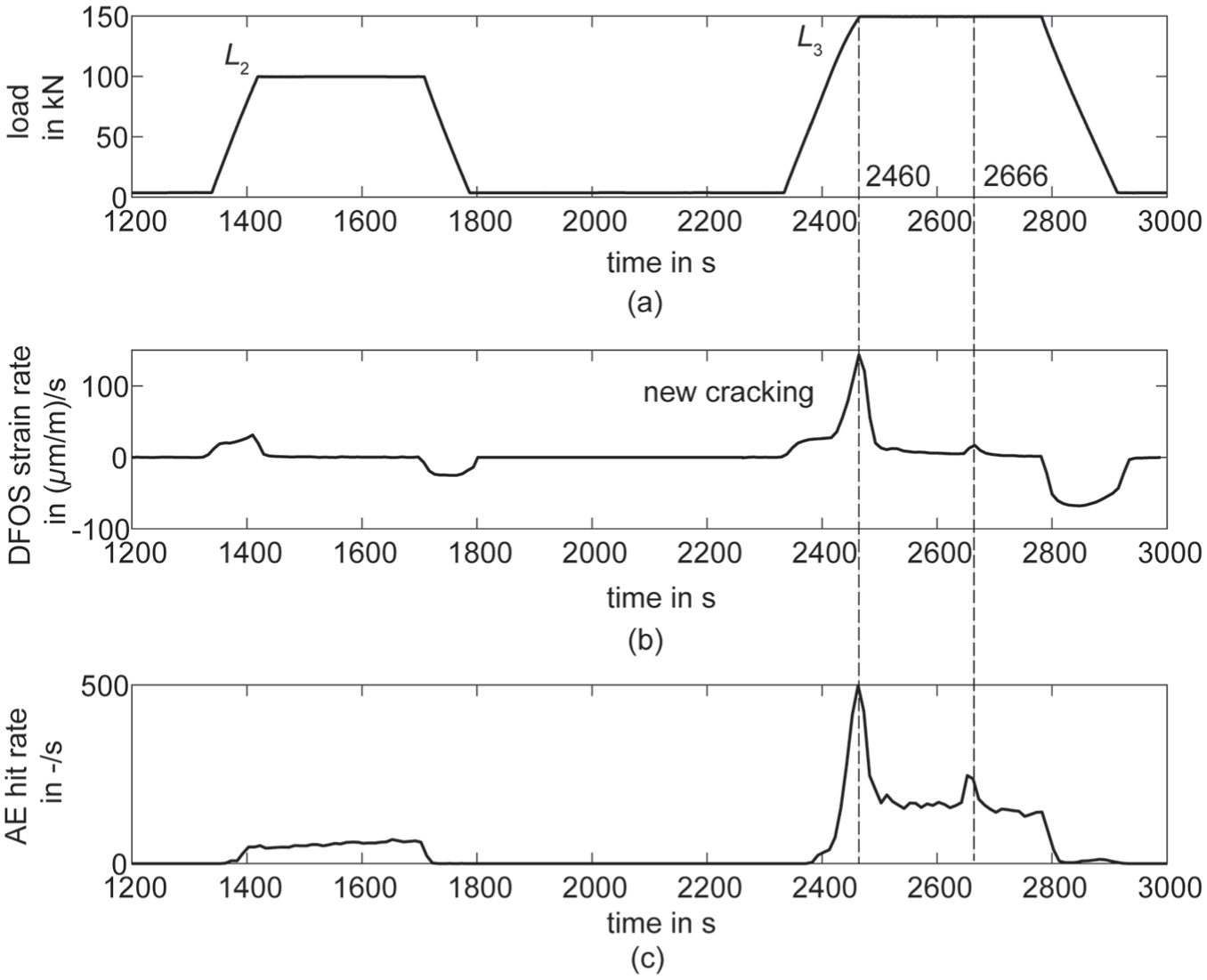
Comparison of DFOS strain rate and AE hit rate for L2 and L3: (a) loading history, (b) DFOS strain rate, and (c) AE hit rate. DFOS: distributed fiber optic sensors; AE: acoustic emission.
When loading to 100 kN (L2), the DFOS strain rate shows a small peak while the AE hit rate does not, which indicates that the activities were not from the formation of new cracks, but possibly from the reopening of existing cracks, which did not generate many AE hits. The AE activities during the sustained load of 100 kN might be due to the noise from the loading machine.
At 150 kN (L3), two distinct peaks were observed at approximately 2460 and 2666 s in both AE hit rate and DFOS strain rate, indicating possible correlations of the two parameters in detecting the formation of new cracks. The reason for detecting peaks at 150 kN, later than the previously identified 130 kN, is that the analysis considered the cumulative strain and AE hits from all cracks. The initial increase at 130 kN, caused by the formation of the first crack, was possibly overshadowed by the larger cumulative increase from multiple cracks forming at higher load levels.
After the crack formation, the DFOS strain rate dropped to nearly zero, while the AE hit rate remained relatively high (around 200 hits per second). This AE activity may be attributed to crack development under sustained loading or the noise from the loading machine. During unloading, the DFOS strain rate became negative due to crack closure, whereas the AE hit rate did not exhibit this behavior.
Discussion
A multi-physical monitoring approach using UPV, AE, and DFOS was proposed for crack monitoring of prestressed concrete girders. The approach suggested three stages of crack detection and monitoring in load testing of the structure. The first stage was detecting existing cracks before loading using UPV. The second stage was verifying the existing cracks in a low-load cycle using DFOS. The load level was below the crack formation force. The third stage was tracking the crack formation and development at higher-load cycles. This section reflects the performance of this combined approach and suggests possible future work.
Stage 1: Detection of existing cracks before loading
The first step involved measuring wave velocities in uncracked concrete to establish a reference for comparison. UPV tests were conducted at three locations: one on the top surface and two on the bottom surface where no cracks were observed. The measured velocities were 3805, 4177, and 4405 m/s, respectively.
Although these values were within the velocity range found in the literature, 85 wave velocity is inherently linked to material properties. Therefore, it is recommended to measure a reference velocity specific to the structures under investigation. The sensor array setup described in “Test 1: Measurement of velocity in uncracked concrete” section could be employed for this purpose. Additionally, in prestressed concrete girders, the stress state may influence wave velocity, as concrete under compression is expected to exhibit higher velocities. Further validation of the effect of stress state on the wave velocity is necessary.
The second step involved measuring the wave velocity distribution in critical regions of the structure, such as the interface between the top cast-in situ layer and the precast girder, or areas critical to failure. This study demonstrated that the wave velocities along ray paths affected by cracks were significantly lower than the reference velocity in uncracked concrete, even after accounting for the spatial variations in concrete velocity. Furthermore, these reduced velocities fell below 3500 m/s, consistent with the empirical threshold suggested in the literature. 63
However, another assumption from the literature 65 was not verified by this article, which was that the influence of a partially-closed crack on the arrival time was much larger than the other sources, such as arrival time picking error. Furthermore, when a partially-closed crack is subjected to compression, which is especially in a prestressed girder, its influence on arrival time remains uncertain. Targeted experiments are needed to quantify this effect and establish a more robust correlation between crack conditions and UPV signals in prestressed concrete girders.
A key limitation of UPV is its inability to distinguish multiple cracks within a single ray path, which was also found in the literature. 30 When accurate crack localization is needed, it is suggested to apply a low-load cycle and perform DFOS strain measurements (see stage 2).
Stage 2: Verification of existing cracks in a low-load cycle
By applying a low-load level before the formation of new cracks, DFOS successfully detected strain peaks at the locations of pre-existing cracks. This finding is crucial, as it demonstrates that crack localization can be achieved without the need for heavy loading. The ability to identify existing cracks under minimal loading reduces the risk of further structural damage.
In contrast, the performance of AE during unloading from this low-load level was not as effective as observed in the literature.66,87 Few AE hits were recorded. This was likely due to two key factors: (1) the smoothened crack surfaces during the service life of the structure, which reduced friction-generated emissions, and (2) the limited relative movement during re-compression, resulting in minimal AE activity. However, in L4 and L5, a significant number of AE hits were recorded during crack re-compression even when unloading from the same 50 kN level. This suggests that re-compression of existing cracks that were partially closed may generate friction. To further develop and validate AE as a method for detecting crack closure or re-compression, dedicated experiments are required to investigate the effects of crack roughness and closure mechanics.
Stage 3: Monitoring crack formation and development in higher-load cycles
Consistent with the findings in the literature, 25 AE proved sensitive in detecting concrete cracking. In this study, AE sensors detected the crack formation at around 130 kN in the constant bending moment zone, much earlier than the appearance of stiffness reduction in the load-deflection curve (170 kN). However, the selection of a threshold for AE hits to determine the onset of cracking remains subjective. This paper applied a fixed threshold of 100 AE hits, which was arbitrarily chosen and not verified. Further validation or refinement of this threshold is needed.
AE detected a possible crack initiation when approaching 200 kN in the web and at the center of the cross-section, which is an area inaccessible to other sensors. This highlights the potential of AE in detecting internal cracks that cannot be observed from the surface. However, this possible cracking in the web could not be verified by other techniques so far.
DFOS detected the crack formation and development through strain rate analysis. A previous concern was that DFOS would be hard to differentiate between new crack formation and existing crack development, as both mechanisms would result in strain increase. Notably, in this study, we found that the strain rate during new crack formation was significantly higher than that during the growth of existing cracks, resulting in a sharper stiffness reduction. In this way, DFOS identified the formation of the first new crack in the constant bending moment zone at 130 kN, which was in line with the AE hit result. This finding suggests the potential to develop a criterion based on strain rate or stiffness reduction rate for differentiating between new crack formation and existing crack growth. Further experimental validation is required to establish a quantitative threshold for practical use.
Additionally, this paper presented an integrated analysis of AE hit rate and DFOS strain rate, revealing a potential correlation when AE hits and DFOS strains were accumulated across all cracks along the girder. Future research could explore localized correlation analysis at individual cracks to further verify this relationship. If confirmed, this correlation could enhance the reliability of crack formation detection by enabling AE and DFOS to cross-validate each other.
To further enhance the integration of AE and DFOS, future studies could explore correlations between DFOS strain and additional AE parameters related to crack formation and progression. These parameters might include signal intensity-based indices (e.g., Historic Index, Severity Index) and frequency-domain features (e.g., peak frequency, partial power distribution). Such an approach could provide deeper insights into crack behavior and further optimize this combined monitoring approach.
Other practical considerations
A key contribution of this article is proposing the use of a minimal load to generate strain peaks at pre-existing crack locations, enabling crack identification. In the case study, this load remained below the decompression force, preventing further damage to the structure. For practical applications, further research could determine whether regular traffic loads are sufficient. If validated, this approach could enable in-service crack detection without traffic disruptions, offering a more cost-effective solution.
Furthermore, practical applications usually deal with complex environments, which bring additional challenges. For instance, environmental noise must be carefully filtered to ensure reliable AE and UPV, which both utilize sound. 88 In cases where noise cannot be fully eliminated, such as traffic noise beneath a viaduct, it is necessary to assess the influence of such noise on AE and UPV. When applying DFOS, the effects of temperature changes on the strain need to be considered.19,89
Additionally, due to resource limitations, such as the available number of sensors and the available time for installation and measurement, it is suggested to prioritize the evaluation of critical locations for implementing the proposed approach. This approach could be used for regions where cracks are not visible during inspection, such as fine cracks or microcracks on the surface and internal damage. Moreover, as noted earlier, this approach is intended specifically for load testing, the sensors can be removed afterward if required.
Conclusions
This article proposed a multi-physical crack monitoring approach for prestressed concrete structures, integrating UPV, AE, and DFOS within a cyclic loading scheme. The combined approach included three key stages: detecting existing cracks before loading with UPV, verifying pre-existing cracks under low-load cycles using DFOS, and tracking crack formation and development at higher-load cycles using DFOS and AE. The key findings and contributions are summarized below.
UPV identified cracks through velocity reduction, compared to the measured reference velocity for uncracked concrete. The reference velocities at three spots of uncracked concrete were 3805, 4177, and 4405 m/s, and the velocities in cracked concrete were below 3500 m/s. Through UPV, potential pre-existing damage was identified in two areas: a localized spot near the top cast-in situ layer and a few spots near the bottom surface.
DFOS verified the existence of cracks by detecting localized strain peaks at a low-load level below the decompression force. The crack locations were found more accurately through the locations of the strain peaks. This also highlights the advantage of detecting existing cracks without heavy loading.
AE detected crack initiation at approximately 130 kN in the constant bending moment zone based on cumulative AE hits, while DFOS identified crack formation at a similar load level based on a rapid local stiffness reduction. Both methods detected cracking significantly earlier than the global stiffness reduction observed in the load-deflection curve, which indicated cracking at 170 kN. This suggests that the girder has never been subjected to a load exceeding the effects of 130 kN in its service life.
Through source localization, AE detected potential crack initiation in the web at the center of the cross-section as the load approached 200 kN, an area inaccessible to other sensors.
DFOS strain rate at new crack formation was higher than that at existing crack growth, leading to more significant local stiffness reduction. This provides a potential criterion for differentiating the two mechanisms.
A preliminary correlation between AE hit rate and DFOS strain rate suggests the potential for cross-validation in crack detection.
Future research could focus on
validating wave velocities in prestressed concrete girders, considering the effect of stress state, presence of cracks, and material properties,
refining AE hit thresholds to establish a more objective criterion for crack detection,
investigating the correlations between AE hit rate and DFOS strain at individual cracks,
exploring the relationships between DFOS strain and other AE parameters, such as signal intensity-based indices and frequency-domain features, to better understand the cracking behavior, and
validating the proposed approach on-site, including investigating the use of traffic loads to induce the strain peaks at pre-existing crack locations (for crack detection) and the influence of the environment on the measurements.
The proposed multi-physical approach enhanced crack monitoring in prestressed concrete girders. It provided high sensitivity to concrete cracking, accurate measurement of crack location and width, differentiation between existing and newly formed cracks, and detection of internal damage that is not visible on the surface. Notably, this approach enabled the detection of existing cracks with no or minimal loading, reducing the need for heavy loading and the risk of further damaging the structure.
Footnotes
Acknowledgements
Special thanks go to Wismar University of Applied Science, in whose structural testing laboratory the described tests were carried out and which contributed significantly to obtaining the described test results by providing a considerable part of the necessary equipment and by providing personnel support and knowledge.
Funding
The authors disclosed receipt of the following financial support for the research, authorship, and/or publication of this article: This work was supported by the Federal Ministry for Digital and Transport, Germany, within the innovation program mFUND [grant number 19FS2013A].
Declaration of conflicting interests
The authors declared no potential conflicts of interest with respect to the research, authorship, and/or publication of this article.
Data availability statement
Data can be shared upon reasonable request.