Damage diagnosis of bridge structures using deep learning strategies: A hybrid neural networks practical tool

Abstract

The accurate identification of damage in bridge structures is critical for ensuring long-term safety and planning timely maintenance interventions. However, environmental noise significantly challenges traditional vibration-based monitoring techniques. The proposed approach develops a deep learning-based intelligent damage classification framework, where stacked denoising autoencoders are employed for noise reduction, and an Inception-enhanced Convolution Neural Networks together with a bi-directional long short-term memory networks are used to automatically extract discriminative spatio-temporal features and classify structural damage states. The performance of the proposed approach is shown by the analysis of a numerical model of the Hanwu cable-stayed bridge in China and field data from the Z24 bridge in Switzerland. The results demonstrate that the proposed method achieves superior classification accuracy and robustness compared to conventional health monitoring models, particularly under noisy conditions, offering a practical tool for bridge health monitoring. The key innovation of this study lies in the integration of learnable denoising and multi-scale spatio-temporal feature extraction within a unified framework, which reduces reliance on hand-crafted preprocessing and significantly enhances robustness under noisy monitoring conditions.

Keywords

bridge health monitoring damage localization denoising autoencoder deep learning convolutional neural networks structural reliability

Introduction

Bridge structures are subject to a wide range of environmental and operational stresses over their long service life, leading to gradual deterioration or sudden damage due to extreme events such as earthquakes, fire, or floods.^1–3 Timely detection and localization of such damage is essential to maintain structural reliability, prevent catastrophic failures, and optimize maintenance planning.

Traditional structural health monitoring (SHM) relies heavily on vibration data collected through acceleration sensors installed at key points across the bridge.^4–6 Early analysis techniques predominantly applied classical signal processing and statistical methods to these data. With the increasing availability of large-scale monitoring data, machine learning (ML) approaches, especially supervised classification techniques, have emerged as promising tools for automated damage identification. For instance, pattern recognition has become one of the most important tools for data processing in SHM.⁷

Initial applications of ML to structural monitoring utilized “shallow” neural networks (NNs) with back-propagation training. While pioneering studies confirmed the feasibility of NNs for damage diagnosis,⁸ those architectures faced challenges such as poor convergence rates, high sensitivity to local minima, and limited capacity to model complex nonlinear relationships.⁹ Furthermore, environmental variations, such as temperature changes or wind loads, often distorted the vibration characteristics of the structures, complicating the diagnosis.

The increase of computational capability has improved the ability to process large, complex, and noisy datasets and moving from simple NN architecture to more complex ones referred as deep NNs. In particular, convolutional NNs (CNNs) and Recurrent NNs (RNNs) have demonstrated the applicability of such technology in capturing spatial and temporal features of structural responses.^10–12 For instance, long short-term memory (LSTM) networks,¹³ that is a specific type of RNN architecture used to overcome the training problem associated with the back-propagation method, have shown excellent performances for real-time monitoring of bridge structure.¹⁴ CNN and LSTM has been combined in the study by Dang et al.¹⁵ for improving SHM capability, but with limited anti-noise capability and extensive manual data handling. In recent years, attention mechanisms and Transformer-based architectures have increasingly been adopted in SHM tasks due to their capability of capturing long-range dependencies in time-series and improving feature interaction modelling. Recent reviews have highlighted the growing dominance of attention/Transformer models and other modern hybrid deep networks across SHM applications.^16,17 Therefore, establishing competitiveness requires positioning proposed models relative to these modern architectures.

Real-world bridge monitoring data are often contaminated by measurement noise and operational variability, which can degrade the reliability of vibration-based diagnosis and increase reliance on extensive manual preprocessing.¹⁸ Although hybrid deep learning architectures have shown promise for capturing spatial and temporal signatures of structural response, their robustness under noisy conditions remains a key limitation for field deployment.¹⁹ More recently, Cai et al.²⁰ developed an intelligent multi-level warning framework for wind-induced vibration of long-span bridges by integrating CNN–LSTM prediction with dimensionality reduction and clustering techniques, and demonstrated its effectiveness using full-scale monitoring data under typhoon conditions. Recent studies combining Inception-enhanced CNNs with LSTM architectures and conventional denoising highlight the potential of multi-scale spatio-temporal learning, but also suggest that noise resilience still depends strongly on the effectiveness of the preprocessing strategy and the transferability of the learned features across datasets.

This study proposes an integrated deep learning framework aimed at improving the practicality and noise resilience of vibration-based bridge damage diagnosis, rather than vibration warning or threshold classification. The framework couples a learnable denoising stage with a hybrid spatio-temporal classifier to reduce dependence on hand-crafted filtering and to enhance generalization across noisy monitoring scenarios.

Specifically, the main contributions are: (1) Noise-robust preprocessing: Environmental and sensor-induced noise in acceleration signals is suppressed using a stacked denoising autoencoder (SDAE)²¹ trained with noise-injected data to learn stable, transferable representations. (2) Multi-scale spatial feature extraction: An enhanced CNN with embedded Inception modules is employed to capture multi-resolution spatial patterns from multi-sensor vibration fields. (3) Bidirectional temporal modelling: A bi-directional LSTM (BiLSTM) layer is integrated to exploit forward and backward dependencies in vibration sequences, improving discrimination of damage scenarios with similar spatial signatures. (4) Cross-context validation: The approach is evaluated using a numerical model of the Hanwu cable-stayed bridge under wind-induced excitation and a field benchmark (Z24 Bridge) to assess both controlled and realistic monitoring conditions.

By integrating learnable denoising with multi-scale spatial and bidirectional temporal feature extraction in a functionally complementary manner, the proposed SDAE–improved CNN (ICNN)–BiLSTM framework advances noise-resilient damage classification and offers a practical pathway toward more reliable bridge health monitoring using standard accelerometer layouts and modest computing resources.

Methodology overview

This section presents an overview of the proposed structural damage diagnosis framework, which integrates signal denoising and feature extraction in a deep learning architecture suitable for application on real-world bridge monitoring data.

Data preprocessing

Acceleration time histories are collected from multiple sensors distributed across the bridge structure. To preserve spatial relationships and capture dynamic characteristics effectively, a sliding window sampling technique segments the vibration signals collected by N sensors into time windows, each forming an input feature map as shown in Figure 1.

Figure 1.

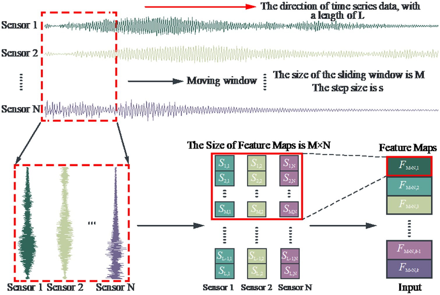
The feature maps of input data.

By setting the window length M and step size s(s < M), the time-series acceleration data is divided into k feature maps of M × N dimension, representing the input of model. In this way, the spatial relationship among signals is preserved, while capturing, the dynamic response characteristics in different time windows. As a good practice in ML, a normalization is applied to scale the data uniformly between [−1,1].

Noise reduction

In SHM, vibration signals collected from bridges are often contaminated by various types of environmental and operational noise such as wind, traffic vibrations, and sensor drift. These noise factors can obscure the subtle changes in vibration patterns that indicate damage. Therefore, effective noise reduction is critical for accurate damage diagnosis.

A wide range of signal-processing-based denoising techniques has been explored in recent SHM studies. For instance, variational mode decomposition has been shown to effectively decompose non-stationary vibration signals into intrinsic mode functions with improved noise separation capability, thereby enhancing damage-sensitive feature extraction.²² Similarly, advanced wavelet-based denoising strategies have demonstrated strong performance in suppressing measurement noise while preserving structural response characteristics.²³ Despite their effectiveness, these approaches typically require careful manual selection of decomposition parameters (e.g., number of modes, penalty factors, wavelet bases, and threshold rules), and they operate independently from the subsequent damage classification stage, which may limit robustness and generalizability under varying monitoring conditions.

A SDAE is employed in this study as an initial data cleaning stage before feature extraction and classification. SDAE is a type of deep learning model that learns to recover clean signals from corrupted inputs through multiple layers of unsupervised learning. At its core, an autoencoder is a NN trained to reconstruct its input after passing it through a compressed hidden representation (a “bottleneck”). However, a DAE takes this idea further as it is training using noisy version of the input and learns to predict the original clean input despite the noise. In SDAEs, several DAEs are connected together layer-by-layer, where each layer progressively learns to extract more higher-level features and suppress noise more effectively at deeper levels.

Compared with traditional fixed-rule denoising techniques, the SDAE provides a data-driven and task-oriented noise reduction mechanism that can be jointly optimized with the downstream damage classification objective. This enables the denoising process to adapt to the statistical characteristics of bridge vibration data under different environmental conditions, while reducing reliance on hand-crafted filtering strategies.

In our model, the training process involves the addition of controlled Gaussian white noise to the original bridge acceleration signals to simulate real-world sensor noise. Each autoencoder layer encodes the noisy input into a compressed representation and decodes it back to approximate the clean original signal. By doing so, it learns features that best separate signal from noise. After training each layer individually, the autoencoders are stacked together into a deep network. The stacked network is subsequently fine-tuned in conjunction with the downstream classifier, allowing the learned denoising representations to directly support robust spatio-temporal feature extraction and damage classification. The entire network is then fine-tuned using supervised learning to optimize overall denoising performance. The final output is a denoised version of the original vibration signals, ready for feature extraction by CNN and BiLSTM networks.

It should be emphasized that the SDAE in this framework is not used as an independent preprocessing filter, but as an integral learnable module jointly optimized with the ICNN–BiLSTM classifier, enabling task-driven noise suppression tailored for damage classification.

Feature extraction

After denoising the vibration signals, it is necessary to identify patterns in the signals that are indicative of damage location and severity. To achieve this, a hybrid deep learning model is designed that leverages the complementary strengths of convolutional and recurrent networks tailored to the specific characteristics of bridge vibration data. Vibration data from bridges is multi-dimensional time-series data where each sensor measures how the structure vibrates over time and different sensors are positioned at distinct locations across the structure.

An ICNN embedded with Inception modules is used to extract spatial features, while a BiLSTM network is used to extract temporal features.

Multi-scale spatial feature extraction

CNN are used for spatial feature extraction. They operate by applying small “filters” (or kernels) that slide across input data to detect local patterns. Each filter can recognize specific vibration features—such as sudden spikes, oscillations, or subtle shifts. Traditional CNNs apply a fixed-size filter across the data. However, in bridge monitoring, damage signatures may occur at multiple scales—both very localized (e.g., a small crack) and more spread out (e.g., gradual settlement). The Inception module²⁴ addresses this by applying multiple convolution filters of different sizes (e.g., small, medium, large) in parallel and combining their outputs into a richer feature set. Inception module can also reduce the dimension of large-size matrix and realize visual information aggregation at different scales. The structure of the Inception module is shown in Figure 2, where: $ConvKernal_i$ symbolizes the ith convolutional layer; $Maxpooling_i$ denotes the ith largest pooling layer; $BN_i$ means the ith batch normalization layer.

Figure 2.

The structure of Inception module.

Temporal feature extraction

RNNs are specialised NN designed to process sequences, where the order of inputs matters.²⁵ They maintain an internal “memory” of previous inputs, allowing them to capture how the signal evolves over time. However, traditional RNNs suffer from issues like short-term memory loss and difficulty learning long-range dependencies.

LSTMs solve these problems by introducing specialized units called “gates” that control the flow of information (e.g., forget gate is used to discard information, input gate to select new information and output gate to decide visible output). Thus, LSTM networks can retain important long-term temporal patterns in the data, which is critical for detecting progressive bridge damage trends.

A standard LSTM looks at the sequence forward in time. However, in structural monitoring, future events (e.g., large oscillations) might help explain earlier vibrations. Hence, BiLSTM is used to process the sequence of data both forward and backward, and learn relationships from both past and future contexts simultaneously. This allows, for instance, to discriminate whether an abnormal oscillation is due to some load conditions or early signs of a failure and this might depend on what happens before and after that event.

In this paper, a two-layer BiLSTM network is designed to enhance the expression ability of the model, as shown in Figure 3. The structural acceleration response signals are fed into the BiLSTM network through the input layer x; the input sample signals pass through the forward LSTM layer to produce output $\vec{h_{t}}$ and the backward LSTM layer to produce output $\overset{\leftarrow}{h_{t}}$ , which together determine the values passed to the hidden layers, resulting in the final BiLSTM output y. In order to prevent the overfitting phenomenon, a dropout layer is introduced after each output of BiLSTM layer. Dropout layer reduces the dependence of the model on specific neurons or features by randomly discarding the output of some neurons, thus improving the generalization ability of the model.

Figure 3.

The structure of BiLSTM. BiLSTM: bi-directional long short-term memory.

Feature fusion: Merging spatial and temporal information

Once spatial features (ICNN branch) and temporal features (BiLSTM branch) are extracted, the two sets of feature vectors are merged into a single comprehensive representation. This fusion layer uses a side-by-side stacking of spatial and temporal feature maps. Finally, the combined features are passed through a fully connected output layer to classify the type and location of damage.

The specific fusion process can be expressed by:

V = V_{ICNN} \oplus V_{BiLSTM}

(1)

where V represents the output of the merge layer, V_ICNN denotes the output of the ICNN layer, capturing spatial features from sensor positions, while V_BiLSTM represents the output of the BiLSTM layer, capturing time-dependent features.

Output layer

As illustrated in Figure 4, the fused feature vector V, obtained by integrating the multi-scale spatial descriptors from the ICNN branch and the bidirectional temporal dependencies captured by the BiLSTM branch, is fed into the output layer to execute final multi-class damage identification. This output layer is designed to transform the joint spatio-temporal representation into class posterior probabilities, enabling a direct mapping from vibration response patterns to discrete structural states.

Figure 4.

Architecture of the ICNN-BiLSTM parallel model. ICNN: improved convolutional neural network; BiLSTM: bi-directional long short-term memory.

In the numerical case study of the Hanwu cable-stayed bridge in “Hanwu cable-stayed bridge simulation” section, the Softmax classifier produces a probability distribution over eight damage levels, corresponding to increasing damage severity. The predicted label is selected using the maximum posterior probability rule, and the associated class probability is retained to support confidence-informed interpretation of the diagnosis. For the Z24 bridge benchmark evaluation in “FE model” section, the same output logic is adopted to classify the pre-defined structural states in the dataset. Although the Z24 damage scenarios differ in physical origin and operational context from the numerical model, the shared output formulation enables a consistent assessment of the framework’s transferability and noise-resilience across simulated and field monitoring environments. This harmonized classification design also facilitates the comparative reporting of confusion matrices and performance metrics across both case studies.

To improve generalization and reduce overfitting, the output block applies one or more fully connected layers with intermediate dropout (typically 50–60%) before the final Softmax stage. This regularized design is particularly important for vibration-based SHM tasks, where limited labelled data, measurement noise, and operational variability may otherwise lead to overly optimistic training performance and reduced robustness at inference time.

Damage classification and evaluation

Following the feature extraction and fusion stages, the final step of the proposed framework is to accurately classify the structural state of the bridge, identifying whether and where damage has occurred. This is achieved through a fully connected dense layer equipped with a Softmax activation function, transforming the learned feature representations into probabilistic outputs over the set of possible damage classes.

Classification mechanism

The output of the fusion block—a vector encoding both spatial and temporal features—is passed into a fully connected layer to map the high-dimensional learned feature space into a lower-dimensional space, corresponding to the number of damage categories by Categorical cross-entropy logistic regression. also known as Softmax.

The Softmax function is applied at the output layer to convert raw prediction scores (“logits”) into normalized probabilities that sum to 1:

P (y = k | x) = p_{k} = \frac{e^{Z_{k}}}{\sum_{j = 1}^{K} e^{Z_{j}}}

(2)

where $z_{k}$ is the output score for class k, K is the total number of damage classes. The class with the highest probability is selected as the predicted damage state. Softmax is particularly suitable for multi-class classification tasks, as is typical in bridge monitoring scenarios involving multiple possible damage locations or severities.

Training strategy

The network is trained using supervised learning with labelled datasets, where each vibration sample is associated with a known damage label (e.g., “undamaged,”“pier settlement,”“tendon rupture”). The loss function used is the categorical cross-entropy, defined as:

L = - \sum_{i = 1}^{N} \sum_{k = 1}^{K} y_{ik} \log (p_{k})

(3)

where N is the number of samples, $y_{ik}$ is the ground truth (1 if sample i belongs to class k otherwise 0), $p_{k}$ is the predicted probability for class k as defined by Equation (2).

The optimization is performed using the Adam (short for Adaptive Moment Estimation) optimizer a standard optimizer used across ML disciplines. The optimiser uses a variant of stochastic gradient descent that adapts the learning rate for each parameter individually. Adam adaptively adjusts the learning rate for each parameter by maintaining an exponentially decaying average of past gradients (first moment) and squared gradients (second moment), offering faster convergence and better resilience to noise compared to standard stochastic gradient descent. Default parameters were used: $β_{1} = 0.9$ , $β_{2} = 0.999$ , and a learning rate of 0.001. Early stopping is employed based on validation loss to prevent overfitting.

Evaluation metrics

To comprehensively assess classification performance, multiple evaluation metrics are employed as shown in Table 1.

Table 1.

Classification metrics.

Metric	Formula	Interpretation
Accuracy	_{$\frac{TP + TN}{TP + TN + FP + FN}$}	Overall fraction of correctly predicted instances.
Precision	_{$\frac{TP}{TP + TN}$}	How many predicted positives are true positives.
Recall (sensitivity)	_{$\frac{TP}{TP + FN}$}	How many actual positives are correctly identified.
F1-score	_{$2 \cdot \frac{Precision \cdot Recall}{Precision + Recall}$}	Harmonic mean of Precision and Recall.

TP: True Positives; TN: True Negatives; FP: False Positives; FN: False Negatives.

In this study, confusion matrices are employed to comprehensively evaluate the classification performance of the proposed framework. Each confusion matrix provides a detailed visualization of the model’s prediction outcomes across different damage states, highlighting correct classifications as well as specific misclassification patterns. Derived metrics such as precision, recall, and F1-score further quantify the model’s reliability, especially emphasizing the importance of minimizing false negatives in bridge health monitoring scenarios

In addition to basic classification metrics, the robustness of the model is tested under conditions of Noisy inputs simulated by adding Gaussian noise to vibration data and different signal-to-noise ratios (SNRs = 5, 10, and 20 dB), and unseen mixed damage states (for generalization capability). Performance degradation is quantified under noise, providing insights into the practical applicability of the method in real-world bridge monitoring, where data quality can be variable.

Baseline models for comparison

To demonstrate the advantages of the proposed framework, its performance is compared against two widely used architectures: Typical CNN model without temporal modelling and BiLSTM model for sequential processing without spatial convolution.

Comparative results shown in “Robustness verification” section show that the proposed model based on SDAE-ICNN-BiLSTM consistently outperforms baselines in accuracy and robustness. The combination of denoising, multi-scale spatial analysis (Inception-CNN), and bi-directional temporal modelling (BiLSTM) provides superior diagnostic capabilities.

Case studies

To evaluate the performance of the proposed SDAE-ICNN-BiLSTM framework, two case studies were conducted: a controlled numerical simulation of the Hanwu cable-stayed bridge in China and a real-world application using field monitoring data from the Z24 Bridge in Switzerland. These studies assess both the classification accuracy and robustness of the proposed method under various damage scenarios and noise conditions.

Hanwu cable-stayed bridge simulation

The Hanwu Bridge is a cable-stayed structure located in Handan, China, as shown in Figure 5. The bridge features a double-plane, prestressed concrete cable system with a main span of 260 m with auxiliary piers on both sides, providing single-hole two-way navigation. It is the longest single pylon cable-stayed bridge in Hebei Province.

Figure 5.

A view of Handan Hanwu Bridge.

FE model

A finite element (FE) model of the bridge was constructed using ANSYS Mechanical APDL with 494 nodes and 418 elements, representing key structural components, including main girders, pylons, and stay cables. The FE model is used to establish the spine model in the spatial bar system model without considering the influence of local internal force, torsion and shear lag effects of the stiffening beam, as shown in Figure 6. It should be noted that this simplified FE model is mainly introduced to illustrate the modelling strategy and the basic dynamic characteristics of the cable-stayed bridge. The subsequent numerical simulations and damage identification analyses in this study are all performed based on the detailed solid model to generate high-fidelity vibration data. The bridge model includes: 26 main girder elements (designated units 1–26), 14 stay cables (designated units 27–40).

Figure 6.

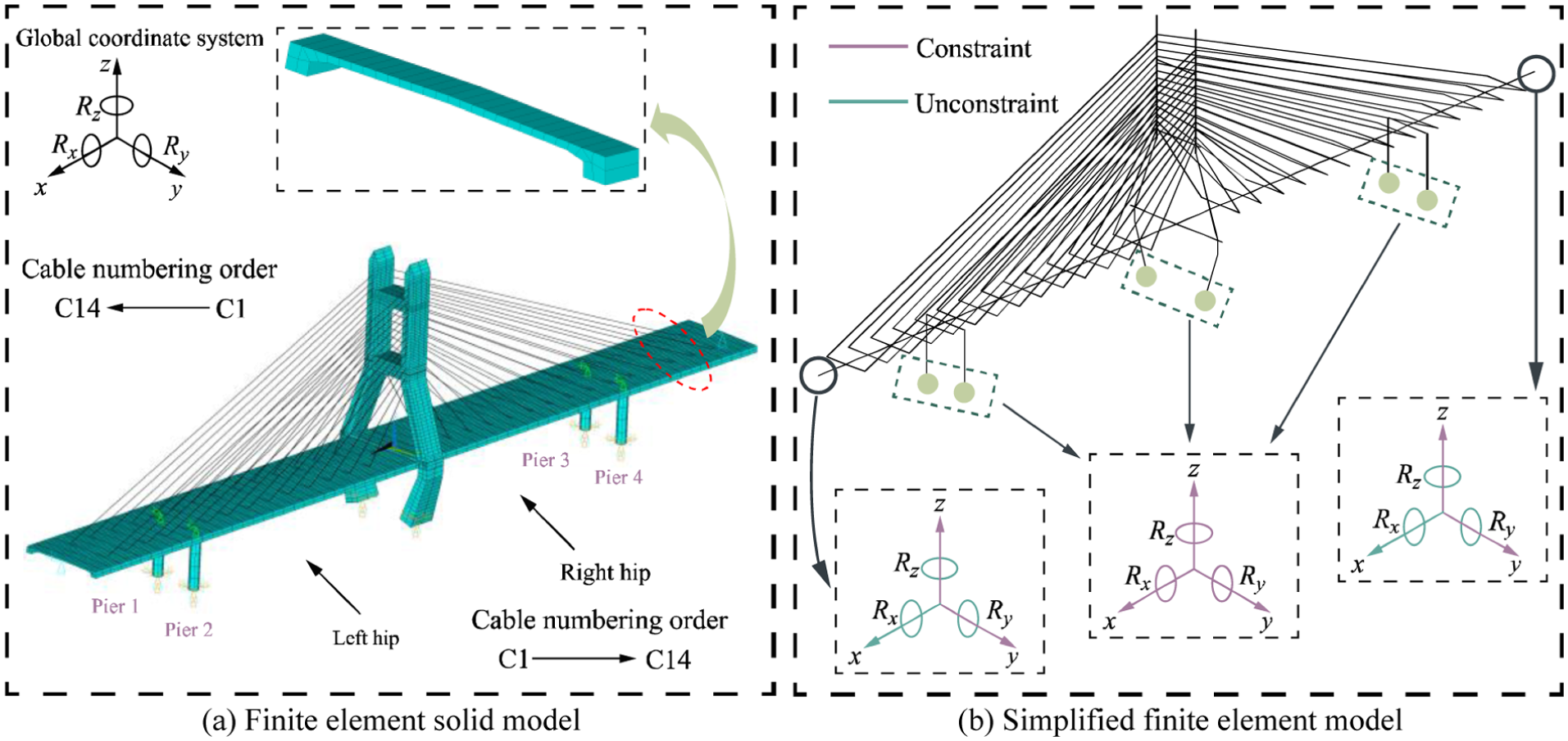
FE model of the Hanwu Bridge cable-stayed bridge: (a) FE solid model and (b) simplified FE model. FE: finite element.

Aerodynamic buffeting loads were simulated using a stochastic fluctuating wind field, modelled via the harmonic superposition method²⁶ ensuring realistic excitation conditions. This model is used to generate vibrational data and allows to evaluate the performance of the proposed SHM approach.

To more accurately simulate the complex loading conditions that bridges experience in real-world environments, this study utilizes pulsating wind loads as excitations to conduct atransient dynamic analysis of the bridge. Subsequently, the training and testing datasets are established based on the acceleration time history collected at specific measurement points.

The wind speed and direction of fluctuating winds vary randomly over time and space, as reported in the study by Xu et al.²⁷ In this study, only the buffeting forces resulting from fluctuating winds are considered. When a bridge structure is subjected to such fluctuating loads, the aerodynamic forces acting on its cross-section include: lift $F_{L}$ , drag $F_{D}$ , and moment $F_{M}$ as shown in Figure 7, where $(j, t)$ represents the node number i and time t, respectively.

Figure 7.

Aerodynamic forces acting on the cross-section due to buffeting wind.

According to the related formulation proposed in the study by Scanlan and Jones,²⁸ the buffeting wind forces acting on the bridge structure can be calculated using the following equations:

F_{D} (j, t) = \frac{1}{2} ρ {\bar{U}}^{2} B [2 \frac{H}{B} C_{D} (α) x_{D} \frac{u (j, t)}{\bar{U}}]

(4)

\begin{matrix} F_{L} (j, t) = - \frac{1}{2} ρ {\bar{U}}^{2} B \\ [2 C_{L} (α) x_{L} \frac{u (j, t)}{\bar{U}} + ({C^{'}}_{L} (α) + \frac{H}{B} C_{D}) x_{L} \frac{w (j, t)}{\bar{U}}] \end{matrix}

(5)

F_{M} (j, t) = \frac{1}{2} ρ {\bar{U}}^{2} B [2 C_{M} (α) x_{M} \frac{u (j, t)}{\bar{U}} + x_{M} {C^{'}}_{M} (α) \frac{w (j, t)}{\bar{U}}]

(6)

where: $u (j, t)$ and $w (j, t)$ are the horizontal and vertical fluctuating wind velocities at node j and time t; $\bar{U}$ represents the mean wind speed; ρ is the air density (1.25 kg/m³); H and B are the mean girder height and width; $x_{D}$ , $x_{L}$ , and $x_{M}$ are the aerodynamic admittance coefficient; $C_{L}$ , $C_{D}$ , and $C_{M}$ are the lift, drag, and moment coefficients, respectively, that depends on the angle of attack $α$ ; finally $C_{M}^{'}$ and $C_{L}^{'}$ are the first-order derivatives of the moment and lift coefficients with respect to the angle of attack.

The cable-stayed bridge under investigation has not undergone wind tunnel experiments; therefore, direct data for various angles of attack are unavailable. To address this limitation, the related aerodynamic parameters are adopted from the literature,²⁹ assuming a wind attack angle of $α = 30^{°}$ along with corresponding aerostatic coefficients and their first-order derivatives shown in Table 2. The harmony superposition method²⁶ is employed to simulate the fluctuating wind field over the cable-stayed bridge. Details of the simulation procedure and numerical values of the model parameters are provided in the Appendix 1.

Table 2.

The numerical values used in the FE model.

Description	Parameters
The lift coefficient	$C_{D} = 0.9378$
The drag coefficient	$C_{L} = - 0.3920$
The moment coefficient	$C_{M} = - 0.05874$
The first-order derivative of moment coefficient with respect to wind attack angle	$d C_{L} / d α = 0.2055$
The first-order derivative of lift coefficient with respect to wind attack angle	$d C_{M} / d α = - 0.1840$

FE: finite element.

Table 3.

Summary of simplified wind speed field.

Wind farm location	orientation	Number of simulation points	Minimum point height (m)	Highest point height (m)
Piers 1 and 2	u	6	0	18
Piers 3 and 4	u	6	0	18
Tower	u	98	0	74
Main beam	u	67	18	18
Main beam	w	67	18	18

Taking nodes 1 and 67 on the main girder as examples (see Figure 8), the time histories of the simulated fluctuating wind speeds are shown in Figure 9. Node 345 is located at the top of the main tower, nodes 1, 20, and 6 are located at different positions in the longitudinal direction of the main beam, and node 149 is located in the middle of the pier. These two nodes are approximately 130 m apart, with node 20 located at midspan. The comparison reveals significant differences in the fluctuation trends between nodes 1 and 67, reflecting the spatial variability of the simulated wind field.

Figure 8.

Node positions in the finite element analysis model diagram.

Figure 9.

Fluctuating wind speed time history of girder: (a) horizon component u and (b) vertical component w.

The three-dimensional wind field for long-span cable-stayed bridges is represented as the sum of a multidimensional, multivariable stationary Gaussian random process in the Cartesian coordinate system, as shown in Equation (7).

{\begin{matrix} U = \bar{U} (z) + u (x, z, t) & \begin{matrix} 0 < x \leq bridge length, \\ 0 < z \leq tower height \end{matrix} \\ v = v (x, z, t) & \begin{matrix} 0 < x \leq bridge length, \\ 0 < z \leq tower height \end{matrix} \\ w = w (x, z, t) & \begin{matrix} 0 < x \leq bridge length, \\ 0 < z \leq tower height \end{matrix} \end{matrix}

(7)

where: the $x$ axis is aligned with the longitudinal direction of the bridge, and the $z$ axis is oriented vertically, both perpendicular to the main flow direction of the wind; $U$ is the speed of the wind flowing from the bridge; $\bar{U} (z)$ is the average wind speed in the mainstream direction; u, v, and w are the fluctuating wind speeds in the transverse, longitudinal, and vertical directions of the bridge; t is the time parameter. According to the structural stress characteristics of the cable-stayed bridge, its pulsating wind field is simplified as follows:

Following the theory of Pulsating Wind Field Simulation presented in the Appendix 1, it is necessary to validate the simulated wind speed histories through power spectral density analysis based on the Kaimal spectra.³⁰ Selected nodes on the main pylon and the no. 1 auxiliary pier were analysed, with the resulting spectra shown in Figure 10. Comparison between the target Kaimal spectrum and the simulated power spectrum indicates a satisfactory match, confirming that the simulated wind field meets the required accuracy for engineering analysis.

Figure 10.

Power spectrum inspection of selected nodes: (a) main tower and (b) auxiliary pier.

After simulating the time history of buffeting wind force, the buffeting wind force at each time step is represented as external loads of nodes in the ANSYS model and the vibration response of the model can be obtained. Finally, the time-varying buffeting forces computed for each node and each time step are applied as external loads in the bridge’s FE model. The resulting dynamic responses are then obtained, providing the basis for damage detection and subsequent ML-based diagnosis.

Simulated vibrational data

Considering the bidirectional symmetry (longitudinal and transverse directions) of the cable-stayed bridge model, this study focuses on the transverse acceleration time histories measured at seven key (virtual) sensor locations under buffeting wind excitation with six accelerometers placed along the main girder, and one accelerometer positioned on the main pylon. The sensor configuration is shown in Figure 11.

Figure 11.

Layout diagram of sensors on Hanwu Bridge, China (unit: meters).

The acceleration at the selected nodes, that is, virtual sensors, is collected with a sampling frequency of 4 Hz for 150 s, resulting in 600 data points per sensor. The full signal is divided into overlapping time windows to create a large number of training samples while maintaining temporal continuity. Each window is treated as an independent sample input for the model.

For each time window, the acceleration signals from different locations are organized into a two-dimensional matrix, where rows represent spatial locations (sensor channels) while channels represent sequential time steps resulting in a [600 × 7] input matrix. This arrangement preserves the spatial and temporal relationships intrinsic to bridge dynamics, allowing the model to capture localized and distributed damage features.

Damage scenario generation

In practical SHM of cable-stayed bridges, damage is often concentrated near critical stress areas such as stay cables that are prone to fatigue, corrosion, or rupture due to sustained tensile stresses and environmental effects and girder sections near cable anchorages due to high bending moments and local stress concentrations. Thus, the damage scenarios designed in this study aim to realistically simulate these phenomena, enabling the model to learn meaningful and practically relevant damage patterns.

Structural damage is simulated as stiffness degradation in the FE model as the reduction in axial $E \times A$ or flexural stiffness $E \times I$ where E is the Young’s modulus, A the cross-sectional area, and I moment of inertia. The stiffness reduction is randomly assigned between 2 and 25% and therefore simulating incipient minor damages as well as serious damage that could compromise bridge integrity. A total of 1000 training samples has been created, as shown in Table 4. The damage affects either single elements (isolated damage), pairs of elements (distributed or simultaneous damage), or mixed configurations involving both stay cables and girder sections.

Table 4.

Training dataset for cable-stayed bridge damage diagnosis grouped by damage type.

Type of damage	Grider		Cable		Mixed damage
Type of damage	Single	Double	Single	Double	Mixed damage
Training number	1–200	201–400	401–600	601–800	801–1000
Damage unit number	1–26 Random damage		27–40 Random damage		1–40 Random damage

To independently evaluate the trained model’s generalization ability, a separate testing dataset of 240 samples is generated as shown in Table 5.

Table 5.

Testing dataset for cable-stayed bridge damage diagnosis.

Damage scenario	Testing sample	Damage units	Labels
Single damage	1–30	Unit 8 only	D1
Single damage	31–60	Cable L3	D2
Double damage	61–90	Unit pairs 12 and 20	D3
	91–120	Unit pairs 8 and 25	D4
	121–150	Cable pairs L5 and L12	D5
	151–180	Cable pairs L7 and L10	D6
Mixed damage	181–210	Girder–cable combinations 14 and L9	D7
Mixed damage	211–240	Girder–cable combinations 19 and L12	D8

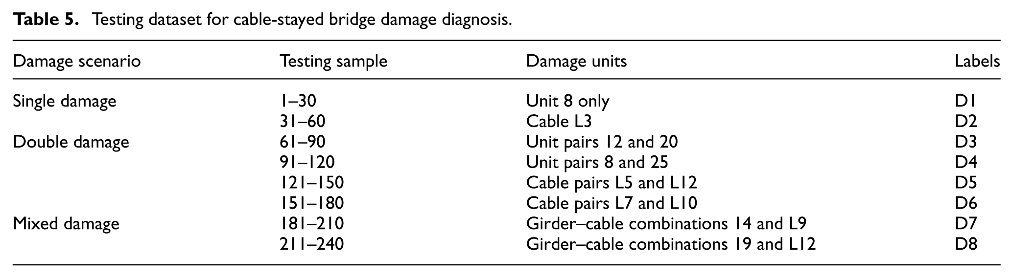
A damage diagnosis test dataset composed of 240 samples has been created to test the performance of the method to detect and locate damages of cable-stayed bridge as shown in Table 5.

Forty possible damage locations are considered: 14 stay cables + 26 girder sections. Damage scenarios are defined using a binary damage vector $D \in {0, 1}^{40}$ where $D_{i} = 1$ indicates damage at unit i while $D_{i} = 0$ indicates healthy state. Each training or testing sample is associated with a unique damage vector.

The sample dataset generation process required for this study is shown in Figure 12.

Figure 12.

Generation process of input samples.

Model training

The proposed hybrid deep learning model as detailed in “Feature extraction” section and shown schematically in Figure 13 is trained and tested using the datasets descripted in “Damage scenario generation” section. The input layer consists of normalized acceleration responses from seven sensors, organized into a matrix of size [600 × 7], representing the acceleration time history signals at seven positions of the cable-stayed bridge.

Figure 13.

Flowchart of the proposed methodology for damage identification of a bridge structure.

All convolution and pooling operations are designed to operate only along the temporal dimension (rows), while maintaining the number of sensor channels unchanged. This is achieved by configuring convolution kernels and pooling windows to have shapes of [n,1], where n controls the extent of temporal aggregation, and the width (sensor dimension) remains constant. As a result, the network can progressively abstract temporal patterns in the vibration signal while preserving the spatial relationships among sensors.

The ICNN is built using a series of standard convolutional layers, followed by an Inception module for distinguishing different types of bridge damage, which may manifest over diverse timescales. The BiLSTM enhances the model’s sensitivity to sequential patterns by allowing information to flow not only forward in time but also backward, providing full context for each moment in the vibration record.

The combined feature representations extracted by the ICNN and BiLSTM branches are then passed through several fully connected (dense) layers. These layers progressively reduce dimensionality and prepare the feature vector for final classification. To mitigate overfitting and improve generalization, dropout layers with varying probabilities (50–60%) are inserted between dense layers. The final output layer applies a softmax activation function, transforming the feature vector into a probability distribution over the possible damage classes. The detailed layer configuration for the ICNN-BiLSTM model is summarized in Table 5.

Baseline model architectures for comparison

For comparative purposes, two baseline models are also developed: A standalone CNN model, which includes convolutional and pooling layers similar to the ICNN branch but without the Inception module and a standalone BiLSTM model, which processes the time-series input directly without prior convolutional feature extraction. The parameters of the CNN and BiLSTM baseline models are detailed in Table 6.

Table 6.

Parameters of ICNN-BiLSTM.

		Values
Layer type		Size	Stride	Filters
CNN	CL_1	[32,1]	[8,1]	16
CNN	ML_1	[2,1]	[1,1]	—
Inception	CL_2	[1,1]	[1,1]	32
	CL_3	[1,1]	[1,1]	32
	CL_4	[1,1]	[1,1]	32
	CL_5	[1,1]	[1,1]	32
	CL_6	[1,1]	[1,1]	64
	CL_7	[1,1]	[1,1]	64
	ML_2	[2,1]	[1,1]	—
BiLSTM	BiLSTM_1	Hidden units		64
BiLSTM	BiLSTM_2	Hidden units		32
Other types	Dropout_1	Probability		50%
	Dropout_2	Probability		50%
	Dropout_3	Probability		60%

CNN: convolutional neural network; ICNN: improved convolutional neural network; BiLSTM: bi-directional long short-term memory; ML: machine learning; CL: convolutional layer.

Both baseline models are configured to have comparable numbers of parameters and training settings to ensure a fair comparison against the hybrid architecture proposed.

It is noted that recent studies in SHM have increasingly adopted more advanced architectures, such as attention-based and Transformer-style models, for time-series analysis.^1,17,31 However, the primary objective of this work is not to exhaustively benchmark against all contemporary architectures, but rather to systematically investigate the effectiveness of the proposed robustness-oriented framework.

Specifically, the selected baseline models as shown in Table 7 represent canonical spatial and temporal learning paradigms in SHM, enabling controlled comparisons to isolate the contributions of the SDAE-based denoising module and the hybrid ICNN–BiLSTM architecture under identical data representations and training conditions. This design choice facilitates fair, reproducible evaluation and avoids confounding performance gains introduced by substantially different model complexities or data requirements.

Table 7.

Parameters of CNN and BiLSTM baseline models.

Model	Layer type	Values
Model	Layer type	Size	Stride	Filters
CNN	CL	[32,1]	[8,1]	16
	ML	[2,1]	[1,1]	—
	Dropout_1	Probability		50%
	Dropout_2	Probability		60%
	Dense	Output size		[40,1]
BiLSTM	BiLSTM_1	Hidden units		64
	BiLSTM_2	Hidden units		32
	Dropout_1	Probability		50%
	Dropout_2	Probability		60%
	Dense	Output size		[40,1]

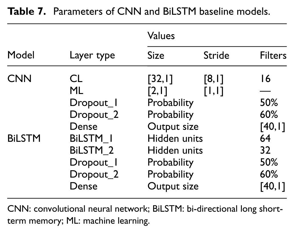
CNN: convolutional neural network; BiLSTM: bi-directional long short-term memory; ML: machine learning.

Training parameters

To optimize the model parameters (weights and biases), the Adam optimizer with the initial learning rate, set to 0.001, is employed. Training is performed using the mini-batch gradient descent method, where a batch of 256 randomly selected training samples is used to estimate the gradient and update the model parameters at each iteration. The model undergoes 500 training epochs, where an epoch corresponds to a complete pass through the entire training set. Throughout training, the cross-entropy loss and classification accuracy are monitored for both the training set and a held-out validation set, allowing for early stopping or hyperparameter adjustment if necessary.

Importantly, data augmentation by noise injection (through the SDAE module) ensures that the training set contains a diverse range of signal-to-noise conditions, thus improving the robustness of the learned feature representations.

Training outcomes and observations

After 500 training epochs, the proposed hybrid model exhibits excellent performance on the training data with a final training accuracy of 98.22% and cross-entropy loss of 0.036. In contrast, the CNN and BiLSTM baseline models achieve accuracies of 95.56 and 91.94%, and loss values of 0.118 and 0.2349, respectively.

The superior convergence behaviour of the proposed model is illustrated by the accuracy and loss curves is shown in Figure 14. These results confirm that the integration of multi-scale temporal convolution (Inception module) with bi-directional sequential modelling (BiLSTM) provides substantial advantages in learning discriminative features from noisy bridge vibration data. Furthermore, the regular use of dropout during training prevents overfitting, ensuring that the model maintains good generalization capabilities when applied to unseen test samples.

Figure 14.

Training process of different models: (a) accuracy and (b) loss function.

A comprehensive evaluation of the proposed models’ diagnostic capabilities is conducted using the confusion matrix shown in Figure 15. The corresponding classification performance metrics (i.e., accuracy, precision, recall, and F1-score) are summarized in Table 8 for each damage category.

Figure 15.

Confusion matrices of different models: (a) ICNN-BiLSTM, (b) CNN, and (c) BiLSTM.

Table 8.

Results of evaluation indicators for different models on the testing set.

Damage labels	Proposed model			CNN			BiLSTM
Damage labels	Precision	Recall	F1	Precision	Recall	F1	Precision	Recall	F1
D1	1	0.9677	0.9836	0.9310	0.9000	0.9153	0.901	0.8333	0.8696
D2	0.9667	1	0.9831	0.7778	0.7568	0.7671	1	1	1
D3	0.9333	0.7778	0.8485	0.8667	0.6500	0.7429	0.7429	0.9286	0.8254
D4	0.7429	0.9286	0.8254	0.8333	0.8929	0.8621	0.75	0.5714	0.6486
D5	0.9310	1	0.9643	0.8438	0.9000	0.8710	0.7576	0.9615	0.8475
D6	0.9286	0.8667	0.8966	0.7586	0.8800	0.8148	0.92	0.7419	0.8214
D7	0.9310	0.9310	0.9310	0.6667	0.9091	0.7692	0.6667	0.8182	0.7347
D8	0.8276	0.8000	0.8136	0.7917	0.6786	0.7308	0.7857	0.7857	0.7857
Accuracy (%)	90.42			80.83			81.25

CNN: convolutional neural network; BiLSTM: bi-directional long short-term memory.

The confusion matrix for the proposed model (Figure 15(a)) reveals that most samples are concentrated along the diagonal, which corresponds to correct classifications. Particularly for the damage labels D2, D5, D6, and D7, the model demonstrates near-perfect classification, with minimal off-diagonal elements indicating misclassification. This high diagonal dominance suggests that the proposed model effectively captures the distinctive features of each damage type, even under complex structural response scenarios.

Quantitatively, the hybrid model achieved an overall accuracy of 90.42%, significantly outperforming the CNN and BiLSTM models, which achieved accuracies of 80.83 and 81.25%, respectively. In terms of precision, recall, and F1-score, the proposed model consistently scores higher across nearly all damage types, showcasing its robustness in both correctly identifying true damage and minimizing false alarms.

In contrast, the confusion matrix for the CNN model (Figure 15(b)) exhibits several noticeable misclassification instances. For example, for damage label D3, there is frequent confusion with label D4, suggesting that the CNN, without temporal context modelling, struggles to distinguish subtle dynamic patterns that differentiate similar damage scenarios. This reflects the inherent limitation of CNNs when processing purely sequential data without mechanisms to capture long-term dependencies.

Similarly, the BiLSTM model (Figure 15(c)) shows good classification performance under simpler damage conditions such as D1 and D2 but suffers performance drops for complex conditions such as mixed damage scenarios such as D7 and D8. This inconsistency indicates that while BiLSTM networks can model time dependencies, they may lack sufficient capacity to fully exploit the spatial features embedded in multi-sensor vibration fields, thus leading to misclassification in more complex conditions.

Overall, the ICNN-BiLSTM model, benefiting from the combined strengths of spatial convolution and bi-directional temporal memory, demonstrates superior classification stability, higher reliability, and lower error rates compared to the standalone CNN and BiLSTM baselines.

Robustness verification

To evaluate performance under realistic monitoring conditions, robustness tests were conducted by artificially contaminating the numerical acceleration signals with Gaussian white noise at three SNR levels: 20, 10, and 5 dB, where lower SNR corresponds to more severe noise contamination. The objective is to quantify the extent to which the proposed framework preserves diagnostic accuracy as signal quality deteriorates.

Noise modelling

Based on Vincent et al.,³² Gaussian noise best models real-world sensor distortions. Therefore, data from the FE model at selected nodes are contaminated with different levels of Gaussian noise. The noisy acceleration $\tilde{a} (j, t)$ at point j and time t is modelled as:

\tilde{a} (j, t) = a (j, t) + γ ε

(8)

where $a (j, t)$ is the original acceleration at node j obtained from the FE model, $γ$ is noise level related to the desired SNR, $ε$ represents a standard normal Gaussian random variable.

Denoising with SDAE

To improve resilience against noise, especially for real-world scenarios, a SDAE is employed to pre-process the normalized signals as explained in “Noise reduction” section. The SDAE consists of multiple DAE layers that compress noisy input into latent features and reconstruct a denoised signal approximation.

SDAE is trained using generated data with different noise levels from Equation (5). SDAE consists of multiple layers of DAEs stacked sequentially, each designed to learn robust features by reconstructing clean signals from noisy inputs. During training, Gaussian noise is added to the input data to simulate real-world disturbances, and the network minimizes the mean squared error between the denoised output and the original clean signal. The SDAE is trained in a layer-wise manner, with each layer learning increasingly abstract representations, and the entire network is fine-tuned afterward. Performance tests demonstrate that the SDAE effectively suppresses noise at various levels of SNR, significantly improving signal quality and the robustness of subsequent damage classification, even under challenging noisy conditions. Quantitative results show that the SDAE reduces reconstruction error rapidly during training and maintains high denoising effectiveness, which enhances the overall reliability of the damage detection framework.

After 500 rounds of iterative training, the loss curve of SDAE model in the training process is obtained, including mean square error (MSE) and root MSE (RMSE), as shown in Figure 16, from which it can be clearly observed that the SDAE model shows superior performance at the early stage of training, and its MSE and RMSE decline rapidly and then gradually tend to be stable in the first 50 rounds of training.

Figure 16.

SDAE training process curve. SDAE: stacked denoising autoencoder.

The acceleration signal reconstructed by SDAE has effectively corrected the baseline drift in the original signal and significantly and improved its stability; moreover, the reconstructed signal greatly reduces noise burrs and mutation points, further improving the purity of the signal, making the entire signal waveform smoother and clearer, and easier for subsequent analysis and processing.

Figure 17 shows that the SDAE reconstruction corrects baseline drift and suppresses high-frequency burrs and abrupt spikes. The denoised signals exhibit smoother waveforms and improved stability, which supports more reliable downstream classification. Specifically, effectively corrects the baseline drift in the original signal and significantly improves the stability of the signal; and the reconstructed signal greatly reduces the noise burrs and mutation points in the noisy signal, further improving the purity of the signal, making the entire signal waveform smoother and clearer, and easier for subsequent analysis and processing.

Figure 17.

Reconstruction results through SDAE under different signal-to-noise ratios: (a) SNR = 5, (b) SNR = 10, and (c) SNR = 20. SDAE: stacked denoising autoencoder; SNR: signal-to-noise ratio.

Result analysis

The robustness evaluation considers the SDAE-ICNN-BiLSTM model with pretrained denoising, a ICNN-BiLSTM without denoising the baseline models CNN and BiLSTM as well. Each model is tested on noisy datasets corresponding to different SNRs. The confusion matrices under these conditions are presented in Figure 18, detailed evaluation metrics are provided in Table 8, and the SDAE-ICNN-BiLSTM model consistently maintains high classification performance across different noise levels, although the accuracy decreases from 90.9% (no noise) to 80.4% with the most severe noise (SNR = 20 dB). Across all damage labels, precision, recall, and F1-scores remain comparatively high, indicating resilience against noise-induced feature corruption. The error bars in Figure 19 represent the standard deviation calculated from eight repeated analyses conducted under each experimental condition. This ensures that the reported results reflect the variability across multiple independent measurements.

Figure 18.

Confusion matrices under varying SNRs for different models: (a) SDAE-ICNN-BiLSTM, (b) ICNN-BiLSTM, (c) CNN, and (d) BiLSTM. SNR: signal-to-noise ratio; SDAE: stacked denoising autoencoder; ICNN: improved convolutional neural network; BiLSTM: bi-directional long short-term memory; CNN: convolutional neural network.

Figure 19.

Prediction accuracy trends of all models under various noise levels.

As expected, the hybrid model without SDAE shows more performance degradation even at low SNRs, although accuracy remains above 80% at SNR = 5 and 10 dB, but it drops sharply to 71.7% at SNR = 20 dB, demonstrating that SDAE plays a critical role in preserving signal integrity under heavy noise. The baseline models (CNN and BiLSTM) exhibit even more pronounced performance declines, with their accuracies fall below 65% under SNR = 10 and 20 dB and increased confusion among damage types.

Table 9 shows the overall prediction accuracy (i.e., the sum of diagonals in the confusion matrix divided by the total number of samples).

Table 9.

Accuracy, precision, recall, and F1-scores for all models across SNR = 5, 10, 20 dB.

Model	Labels	SNR = 5				SNR = 10				SNR = 20
Model	Labels	Precision	Recall	F1	Accuracy	Precision	Recall	F1	Accuracy	Precision	Recall	F1	Accuracy
1	D1	0.848	0.933	0.89	0.871	0.848	0.933	0.89	0.841	0.727	0.960	0.83	0.804
	D2	0.824	0.933	0.88		0.964	0.844	0.90		0.818	0.900	0.86
	D3	0.897	0.867	0.88		0.844	0.871	0.86		0.735	0.833	0.78
	D4	0.844	0.900	0.87		0.788	0.839	0.81		0.813	0.867	0.84
	D5	0.962	0.833	0.89		0.833	0.833	0.83		0.815	0.759	0.79
	D6	0.862	0.833	0.85		0.889	0.800	0.84		0.885	0.676	0.77
	D7	0.867	0.867	0.87		0.821	0.793	0.81		0.889	0.706	0.79
	D8	0.889	0.800	0.84		0.759	0.815	0.79		0.786	0.786	0.79
2	D1	0.824	0.933	0.88	0.858	0.719	0.852	0.78	0.800	0.703	0.867	0.78	0.717
	D2	0.906	0.806	0.85		0.769	0.732	0.75		0.722	0.867	0.79
	D3	0.963	0.765	0.85		0.742	0.767	0.75		0.676	0.767	0.72
	D4	0.900	0.931	0.92		0.897	0.867	0.88		0.793	0.767	0.78
	D5	0.960	0.857	0.91		0.800	0.857	0.83		0.800	0.667	0.73
	D6	0.781	0.806	0.79		0.848	0.824	0.84		0.625	0.667	0.65
	D7	0.885	0.885	0.88		0.778	0.808	0.79		0.708	0.567	0.63
	D8	0.706	0.923	0.80		0.895	0.708	0.79		0.739	0.567	0.64
3	D1	0.818	0.900	0.86	0.821	0.758	0.893	0.82	0.738	0.875	0.700	0.78	0.654
	D2	0.893	0.833	0.86		0.694	0.862	0.77		0.815	0.733	0.77
	D3	0.813	0.867	0.84		0.629	0.733	0.68		0.741	0.667	0.70
	D4	0.857	0.800	0.83		0.786	0.759	0.77		0.731	0.633	0.68
	D5	0.862	0.833	0.85		0.676	0.697	0.69		0.538	0.700	0.61
	D6	0.719	0.767	0.74		0.778	0.778	0.78		0.543	0.633	0.58
	D7	0.750	0.800	0.77		0.909	0.606	0.73		0.679	0.633	0.66
	D8	0.885	0.767	0.82		0.760	0.613	0.68		0.471	0.533	0.50
4	D1	0.926	0.714	0.81	0.783	0.833	0.641	0.72	0.713	0.724	0.700	0.71	0.625
	D2	0.839	0.867	0.85		0.735	0.833	0.78		0.677	0.700	0.69
	D3	0.758	0.833	0.79		0.759	0.595	0.67		0.690	0.667	0.68
	D4	0.676	0.767	0.72		0.957	0.733	0.83		0.559	0.633	0.59
	D5	0.750	0.800	0.77		0.724	0.656	0.69		0.600	0.600	0.60
	D6	0.880	0.733	0.80		0.541	0.741	0.63		0.600	0.600	0.60
	D7	0.840	0.750	0.79		0.679	0.792	0.73		0.586	0.567	0.58
	D8	0.667	0.815	0.73		0.567	0.810	0.67		0.571	0.533	0.55

SNR: signal-to-noise ratio.

The SDAE-ICNN-BiLSTM model consistently maintains high classification performance across different noise levels, although the accuracy decreases from 90.9% (no noise) to 80.4% with the highest level of noise (SNR = 20 dB). Across all damage labels, precision, recall, and F1-scores remain comparatively high, indicating resilience against noise-induced feature corruption. The error bars in Figure 19 represent the standard deviation calculated from eight repeated analyses conducted under each experimental condition. This ensures that the reported results reflect the variability across multiple independent measurements.

As expected, the hybrid model without SDAE shows more performance degradation even at low SNRs although accuracy remains above 80% at SNR = 5 and 10 dB but it drops sharply to 71.7% at SNR = 20 dB, demonstrating that SDAE plays a critical role in preserving signal integrity under heavy noise. The baseline models (CNN and BiLSTM) exhibit even more pronounced performance declines with their accuracies fall below 65% under SNR = 10 and 20 dB and increased confusion among damage types.

The superior performance of the SDAE over the ICNN-BiLSTM in noise-free conditions is primarily due to its ability to learn more robust and generalized features through unsupervised denoising training. This process allows the SDAE to capture essential signal characteristics that are less sensitive to variations in initial weights and training randomness, resulting in better feature representations. Consequently, even without external noise, the SDAE-enhanced model can achieve higher accuracy, as it benefits from more effective feature extraction and initialization, providing an inherent advantage over models trained solely in supervised mode.

These findings clearly highlight that noise robust feature extraction and denoising are crucial for maintaining diagnostic accuracy in real-world SHM applications, where environmental noise is inevitable.

Although low-dimensional visualization techniques such as t-SNE are sometimes used to qualitatively illustrate feature separability, this study prioritizes confusion-matrix-based analysis and noise-level-controlled evaluations, which provide more direct and reproducible evidence of classification robustness and practical diagnostic reliability under realistic monitoring conditions.

From a broader methodological perspective, recent studies in SHM have increasingly explored attention-based and Transformer-style architectures for time-series modelling, motivated by their capability to capture long-range dependencies and complex feature interactions. Representative examples include Transformer-based damage detection frameworks and attention-enhanced hybrid networks, which have demonstrated competitive performance on various SHM benchmarks.

While such models are effective in many scenarios, their performance is often contingent on large-scale training data, careful hyper-parameter tuning, and relatively clean signal conditions. In contrast, the present study emphasizes robustness-oriented design by explicitly incorporating a learnable denoising stage prior to spatio-temporal feature extraction. The experimental results indicate that the proposed SDAE–ICNN–BiLSTM framework maintains stable performance under severe noise contamination, which is a critical requirement for practical field monitoring. The experimental benchmark presented in this study adopted well established SHM baseline architectures (i.e., CNN and BiLSTM) in order to perform a clearer evaluation of the contribution of the proposed denoising and hybrid spatio-temporal learning framework under controlled conditions.

To contextualize the proposed approach within the rapidly evolving SHM literature, a comparative summary of representative modern deep learning architectures is provided in Table 10. Rather than reporting direct numerical comparisons, Table 10 highlights the modelling paradigms, typical application scopes, and practical considerations of recent state-of-the-art methods, thereby clarifying the complementary role of the proposed framework with respect to existing attention and Transformer-based approaches.

Table 10.

Representative modern deep learning architectures for SHM.

Architecture category	Representative model/strategy	Typical SHM applications	Key strengths	Practical considerations	Reference
Attention-based CNN	CNN with channel or temporal attention	Damage classification, anomaly detection	Enhanced feature weighting and interpretability	Sensitive to noise; attention weights may fluctuate under low SNR	¹⁷
Transformer-based models	Temporal Transformer/Vision Transformer variants	Long-term time-series modelling, multi-sensor SHM	Strong capability for modelling long-range dependencies	High data demand; computationally intensive; robustness under noise is not always guaranteed	¹⁶
CNN–RNN hybrid models	CNN + LSTM/BiLSTM	Vibration-based damage diagnosis	Joint spatial–temporal feature extraction	Performance degrades under severe noise without explicit denoising	¹⁷
Hybrid models with explicit robustness design	SDAE + ICNN + BiLSTM (this study)	Noisy vibration-based damage identification	Noise-insensitive representation learning; stable performance under low SNR	Slightly increased model complexity due to denoising module	This work

SHM: structural health monitoring; CNN: convolutional neural network; RNN: recurrent neural network; LSTM: long short-term memory; ICNN: improved convolutional neural network; SDAE: stacked denoising autoencoder; BiLSTM: bi-directional long short-term memory.

Ablation study

To quantitatively evaluate the contribution of each module in the proposed framework, a targeted ablation study was conducted, with particular emphasis on the SDAE module, designed to enhance noise robustness for SHM applications. Specifically, the full model was compared with a reduced configuration in which the SDAE module was removed while the ICNN and BiLSTM components remained unchanged. This comparison directly assesses whether the performance improvement under noisy conditions originates from the SDAE-based denoising mechanism, rather than from the classifier’s complexity.

As shown in Table 11, the removal of the SDAE module leads to a noticeable degradation in classification performance, especially under noisy conditions. Although the ICNN–BiLSTM classifier remains capable of learning discriminative features, its performance is more sensitive to noise without the SDAE-based feature denoising stage.

Table 11.

Ablation study of the proposed framework.

Model configuration			Accuracy
SDAE	ICNN	BiLSTM	SNR = 5	SNR = 10	SNR = 20
√	√	√	0.871	0.841	0.804
×	√	√	0.858	0.800	0.717
√	√	×	0.844	0.794	0.751

SDAE: stacked denoising autoencoder; ICNN: improved convolutional neural network; BiLSTM: bi-directional long short-term memory; SNR: signal-to-noise ratio.

These results confirm that the SDAE module plays a critical role in improving the robustness of the proposed method, rather than the performance gain being solely attributed to a more complex classifier.

Damage identification in the Z24 Bridge

Overview of the Z24 Bridge

The Z24 Bridge was a reinforced concrete highway bridge located near Koppigen, connecting Koppigen and Utzenstorf in Switzerland.³³ It served as part of the national highway system before being decommissioned in 1998. However, before its decommissioning, the bridge was subjected to a unique full-scale damage experiment under controlled conditions, including pier settlement, foundation tilting, concrete spalling, anchor head failure, prestressing tendon rupture, making it one of the most extensively instrumented and studied bridges for SHM research. The bridge was a three-span, prestressed concrete box girder bridge that spanned a total length of 60 m. Figure 20 illustrates the elevation view, cross-section, and sensor layout of the bridge.

Figure 20.

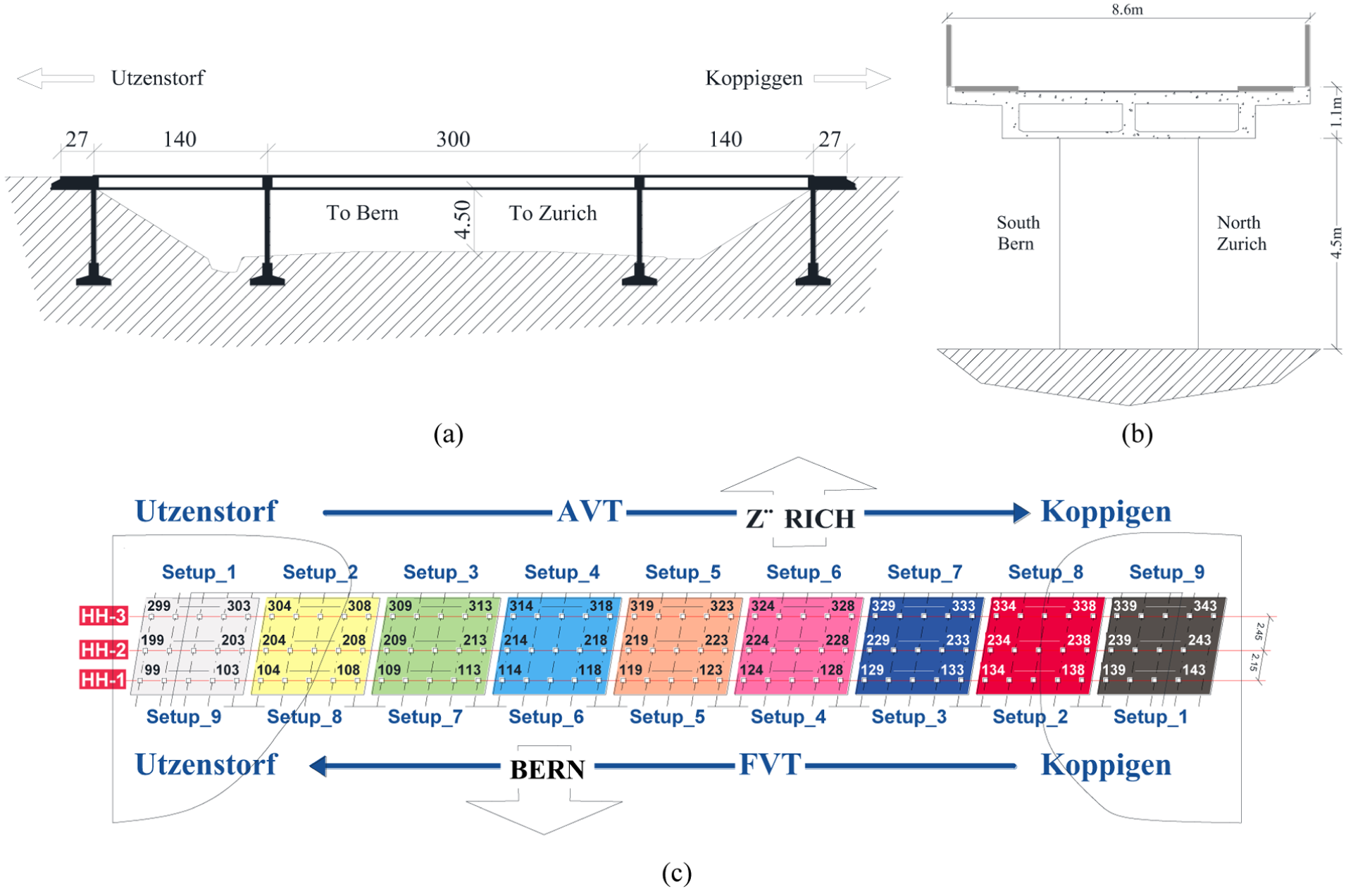
The Z24 Bridge: (a) longitudinal section and main dimensions, (b) close-up of the deck and one pier, and (c) sensor floor plan.

Health monitor dataset

The Z24 Bridge dataset consists of long-term monitoring records collected over a 10-month period, from November 1997 to September 1998. The monitoring campaign was structured into two distinct phases to systematically study both environmental and damage-induced variations in the bridge’s dynamic behaviour.

In the first phase (November 1997 to August 1998), data acquisition was carried out while the bridge remained in an undamaged state. During this phase, the primary objective was to capture the natural variability of the bridge’s vibration characteristics under operational conditions. Environmental factors such as temperature fluctuations, wind loads, and humidity changes were found to significantly influence the modal parameters, especially natural frequencies and damping ratios. This phase provided a comprehensive baseline characterization of the healthy structure, accounting for ambient environmental variability.

The second phase (August to September 1998) introduced a series of controlled damage scenarios. Various structural modifications were intentionally applied to simulate typical bridge deterioration mechanisms. After each damage intervention, the dynamic response of the bridge was recorded under ambient excitation. This phase is particularly valuable for damage identification studies, as it enables direct comparison between undamaged and damaged states under realistic operational conditions.

In the present study, the second-phase dataset is selected to evaluate the performance of the proposed SDAE-ICNN-BiLSTM model for damage detection and classification, as it contains a comprehensive set of labelled damage scenarios corresponding to different severities and types.

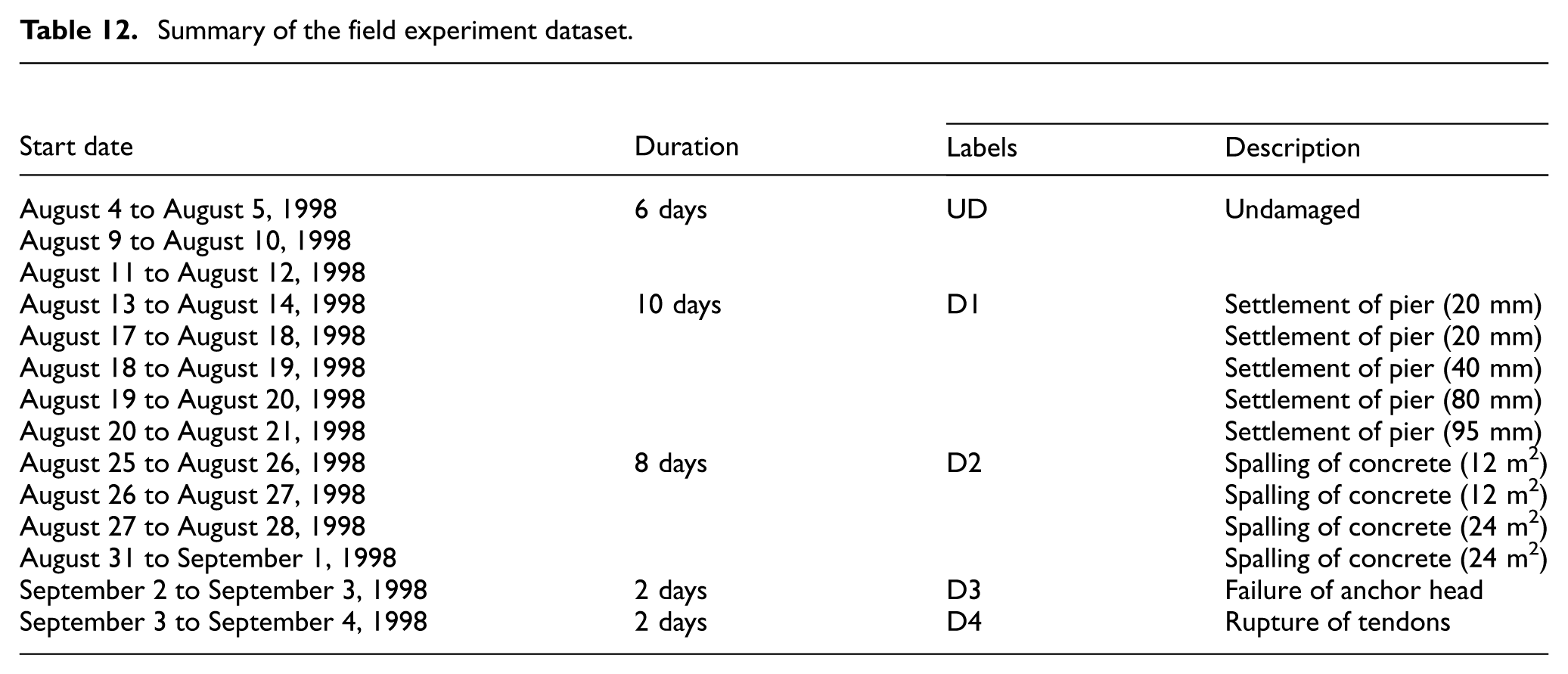
The damage conditions introduced into the Z24 Bridge can be categorized into five distinct types and used for classification purposes, as summarized in Table 12:

undamaged condition (baseline reference),

pier settlement (vertical displacement of bridge supports),

concrete spalling (surface material degradation exposing reinforcement),

anchor head failure (loss of post-tensioning anchor efficiency),

tendon rupture (fracture of internal prestressing cables).

Table 12.

Summary of the field experiment dataset.

Start date	Duration
Start date	Duration	Labels	Description
August 4 to August 5, 1998	6 days	UD	Undamaged
August 9 to August 10, 1998
August 11 to August 12, 1998
August 13 to August 14, 1998	10 days	D1	Settlement of pier (20 mm)
August 17 to August 18, 1998			Settlement of pier (20 mm)
August 18 to August 19, 1998			Settlement of pier (40 mm)
August 19 to August 20, 1998			Settlement of pier (80 mm)
August 20 to August 21, 1998			Settlement of pier (95 mm)
August 25 to August 26, 1998	8 days	D2	Spalling of concrete (12 m²)
August 26 to August 27, 1998			Spalling of concrete (12 m²)
August 27 to August 28, 1998			Spalling of concrete (24 m²)
August 31 to September 1, 1998			Spalling of concrete (24 m²)
September 2 to September 3, 1998	2 days	D3	Failure of anchor head
September 3 to September 4, 1998	2 days	D4	Rupture of tendons

The vibration data was primarily acquired using accelerometers at a sampling frequency of 100 Hz. Each recording session captured a continuous vibration time history over a duration of 660 s, resulting in a total of 65,536 data points per sensor channel.

All recorded acceleration signals underwent a normalization process. The normalized acceleration signals were divided into 64 non-overlapping fixed-length segments of 10.24 s each, corresponding to 1024 data points per segment as illustrated in Figure 21.

Figure 21.

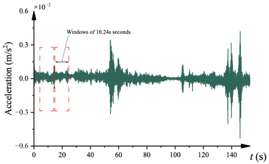
Data segmentation from the Z24 Bridge acceleration.

Following the segmentation process, the complete field experiment dataset consisted of 320 samples. To facilitate model training and evaluation, the dataset was partitioned based on monitoring phases and structural conditions rather than randomly at the individual segment level. Samples generated from the same monitoring phase were grouped and assigned exclusively to either the training or testing subset, with 80% of the samples (256 samples) used for training and the remaining 20% (64 samples) reserved for testing. This scenario-based partitioning helps reduce potential information leakage caused by temporal correlation between adjacent vibration segments. Each training sample was associated with a damage label based on the predefined conditions outlined in Table 12.

The structured dataset for model input was formatted as a three-dimensional tensor with dimensions [256, 1024, 5], where 256 represents the number of training samples, 1024 the number of time points per sample, and 5 the measured features corresponding to sensors within the voltage range of 204–238 V.³⁴ Each group of five sensors was treated as a single input set. Training was conducted independently for the proposed model and the baseline models as shown in “Hanwu cable-stayed bridge simulation” section. The selected values of the hyperparameters are shown in Table 6, and each model was trained over 200 epochs using a learning rate of 0.001 and a mini-batch size of 256.

Results and discussion

The classification performance was evaluated using the testing subset of the dataset, comprising 64 samples (20% of the total dataset). The confusion matrices illustrating the classification results of the ICNN-BiLSTM and conventional models under different damage scenarios are presented in Figure 22.

Figure 22.

Confusion matrix: (a) regular CNN model, (b) regular BiLSTM model, (c) proposed ICNN–BiLSTM model, and (d) SDAE-ICNN-BiLSTM model. CNN: convolutional neural network; ICNN: improved convolutional neural network; SDAE: stacked denoising autoencoder; BiLSTM: bi-directional long short-term memory.

The results clearly demonstrate that the proposed SDAE-ICNN-BiLSTM model significantly outperforms the baseline models in accurately identifying and classifying various damage types under noisy conditions. It maintains high classification accuracy, robustness, and stability across different SNRs, even at low SNR levels such as 5 dB. Furthermore, the integration of the DAE markedly enhances the model’s ability to extract noise-robust features, which is reflected in the superior performance compared to the models without denoising. These findings confirm that the proposed approach is highly effective for real-world bridge health monitoring, where measurement noise and environmental variability are prevalent.

Further quantitative evaluation metrics are summarized in Table 13. Comparative analysis shows that the ICNN-BiLSTM consistently outperforms the conventional CNN and BiLSTM architectures across all metrics, confirming its superior capability for robust, multi-class structural damage.

Table 13.

Performance of classification models using field experiment (validation) datasets.

Classification model	Case	Accuracy (%)	Precision	Recall	F1
SDAE-ICNN-BiLSTM	UD	95.31	0.94	1	0.97
	D1		1	0.92	0.96
	D2		1	0.93	0.96
	D3		0.91	1	0.95
	D4		0.92	1	0.96
ICNN-BiLSTM	UD	93.75	1	0.8	0.89
	D1		1	1	1
	D2		0.82	0.93	0.87
	D3		1	1	1
	D4		0.87	1	0.93
CNN	UD	89.06	1	0.56	0.71
	D1		1	1	1
	D2		0.68	0.93	0.79
	D3		1	1	1
	D4		0.92	0.85	0.88
BiLSTM	UD	81.25	0.8	0.31	0.45
	D1		0.93	1	0.97
	D2		0.58	0.92	0.71
	D3		1	1	1
	D4		0.875	0.88	0.875

CNN: convolutional neural network; ICNN: improved convolutional neural network; SDAE: stacked denoising autoencoder; BiLSTM: bi-directional long short-term memory.

The application of the SDAE-ICNN-BiLSTM model to the Z24 bridge dataset yielded promising results on real-case dataset with an overall test accuracy exceeded 85%, with particularly strong performance in distinguishing between healthy and early-stage damage states identification.

Conclusions

In this paper, a structural damage identification methodology based on an integrated deep NN architecture was proposed, combining a SDAE, CNNs with Inception modules, and a BiLSTM network. The model was specifically designed to analyse typical sensor responses such as the acceleration responses collected from the girder and pylon of a cable-stayed bridge subjected to wind-induced excitations. One notable feature of the proposed approach is that it avoids the need for specialized local sensors (e.g., cable- specific instrumentation) and extensive modal identification preprocessing, making real-time structural health assessment feasible even on standard computing platforms and laptops.

Several key findings emerge from the study: Wind-induced ambient vibrations provide a practical and non-invasive source of dynamic response data for damage detection. By placing a limited number of accelerometers at strategic locations, continuous bridge monitoring can be achieved without disrupting traffic operations or incurring substantial economic costs. Under noiseless or low-noise conditions, the proposed ICNN-BiLSTM architecture demonstrates excellent damage identification performance and significantly outperforms traditional CNN models, which achieve a lower training accuracy.

The integration of the SDAE module significantly enhances the model’s resilience to measurement noise in the numerical model. Even under adverse noise environments with signal-to-noise ratios as low as 20 dB, the model demonstrates reliable identification accuracy. This result highlights the robust feature extraction and denoising capabilities of the model, making it effective for real-world applications where noise is often present, though further validation in physical environments is required.

The proposed framework’s applicability was evaluated using real-world field data from the Z24 Bridge dataset. While the analysis of the Z24 Bridge data provides valuable insights, the identification of damage scenarios in this complex, environmentally variable setting did not fully validate the robustness of the model as initially stated. Nonetheless, the results from the numerical model, in conjunction with the Z24 dataset, indicate the potential of the framework for future deployment in bridge health monitoring systems, subject to further testing and refinement as well a comprehensive benchmarking against a wider set of Transformer-based models.

Model interpretability is also an important aspect for practical SHM applications. Future research could explore interpretability-oriented techniques, such as feature visualization or explanation methods (e.g., Gradient-weighted Class Activation Mapping (Grad-CAM) or similar approaches), to provide deeper insights into the decision-making mechanisms of the proposed deep learning framework.

Footnotes

Appendix 1 Acknowledgements

The authors wish to express their sincere gratitude to the sponsors.

ORCID iDs

ChangSheng Xiang

Hua Zhao

GuoJi Wu

Edoardo Patelli

Funding

The authors disclosed receipt of the following financial support for the research, authorship, and/or publication of this article: This research work was jointly supported by the National Natural Science Foundation of China (grant no. 51868045) and Gansu Province Science and Technology Support Program Science and Technology Innovation Talent Plan Project (grant no. 25RCKA014).

Declaration of conflicting interests

The authors declared no potential conflicts of interest with respect to the research, authorship, and/or publication of this article.

Data availability statement

Data will be made available on request.

References

Zhuang

Chen

Jin

, et al. A review of computer vision-based structural deformation monitoring in field environments. Sensors 2022; 22: 3789. https://doi.org/10.3390/s22103789

W-L

Wang

, et al. Research on fatigue damage correction coefficient of main truss members of railway suspension bridges. Alex Eng J 2024; 89: 83–97. https://doi.org/10.1016/j.aej.2024.01.005

Yan

. Bridge safety monitoring and evaluation based on hesitant fuzzy set. Alex Eng J 2022; 61: 1183–1200. https://doi.org/10.1016/j.aej.2021.06.101

Hann

Singh-Levett

Deam

, et al. Real-time system identification of a nonlinear four-story steel frame structure—application to structural health monitoring. IEEE Sens J 2009; 9: 1339–1346. https://doi.org/10.1109/JSEN.2009.2022434

Salehi

, et al. Integrated structural health monitoring in bridge engineering. Autom Constr 2022; 136: 104168. https://doi.org/10.1016/j.autcon.2022.104168

Ahmadian

Beheshti Aval

Noori

, et al. Comparative study of a newly proposed machine learning classification to detect damage occurrence in structures. Eng Appl Artif Intell 2024; 127: 107226. https://doi.org/10.1016/j.engappai.2023.107226

Jain

Duin

Mao

. Statistical pattern recognition: a review. IEEE Trans Pattern Anal Mach Intell 2000; 22: 4–37. https://doi.org/10.1109/34.824819

Venkatasubramanian

Chan

. A neural network methodology for process fault diagnosis. AIChE J 1989; 35: 1993–2002. https://doi.org/10.1002/aic.690351210

Zhu

G-Q

, et al. Data mining with big data. IEEE Trans Knowl Data Eng 2013; 26: 97–107.

10.

Avci

Abdeljaber

Kiranyaz

, et al. A review of vibration-based damage detection in civil structures: from traditional methods to Machine Learning and Deep Learning applications. Mech Syst Signal Process 2021; 147: 107077. https://doi.org/10.1016/j.ymssp.2020.107077

11.

Xiong

Kong

Xiong

, et al. Zero-shot knowledge transfer for seismic damage diagnosis through multi-channel 1D CNN integrated with autoencoder-based domain adaptation. Mech Syst Signal Process 2024; 217: 111535. https://doi.org/10.1016/j.ymssp.2024.111535

12.

Bao

Liu

. A mechanics-informed neural network method for structural modal identification. Mech Syst Signal Process 2024; 216: 111458. https://doi.org/10.1016/j.ymssp.2024.111458

13.

Van Houdt

Mosquera

Nápoles

. A review on the long short-term memory model. Artif Intell Rev 2020; 53: 5929–5955. https://doi.org/10.1007/s10462-020-09838-1

14.

Sharma

Sen

. Real-time structural damage assessment using LSTM networks: regression and classification approaches. Neural Comput Appl 2023; 35: 557–572. https://doi.org/10.1007/s00521-022-07773-6

15.

Dang

Tran-Ngoc

Nguyen

, et al. Data-driven structural health monitoring using feature fusion and hybrid deep learning. IEEE Trans Autom Sci Eng 2021; 18: 2087–2103. https://doi.org/10.1109/TASE.2020.3034401

16.

Spencer

Sim

S-H

Kim

, et al. Advances in artificial intelligence for structural health monitoring: a comprehensive review. KSCE J Civ Eng 2025; 29: 100203. https://doi.org/10.1016/j.kscej.2025.100203

17.

Cha

Ali

Lewis

, et al. Deep learning-based structural health monitoring. Autom Constr 2024; 161: 105328. https://doi.org/10.1016/j.autcon.2024.105328

18.

Chen

Zhou

Wang

, et al. Deployment of a smart structural health monitoring system for long-span arch bridges: a review and a case study. Sensors 2017; 17: 2151. https://doi.org/10.3390/s17092151

19.

Chi

Cai

Ren

, et al. Damage location diagnosis of frame structure based on wavelet denoising and convolution neural network implanted with Inception module and LSTM. Struct Health Monit 2024; 23: 57–76. https://doi.org/10.1177/14759217231163777

20.

Cai

Liu

Guo

, et al. Investigation on nonstationary wind effects and intelligent multi-level warning method for wind-induced vibration of bridges. Structures 2026; 84: 111112. https://doi.org/10.1016/j.istruc.2026.111112

21.

Jia

Ul Haq

. Fault diagnosis based on SPBO-SDAE and transformer neural network for rotating machinery. Measurement 2022; 188: 110545. https://doi.org/10.1016/j.measurement.2021.110545

22.

Wang

Maghareh

, et al. Effective structural impact detection and localization using convolutional neural network and Bayesian information fusion with limited sensors. Mech Syst Signal Process 2025; 224: 112074. https://doi.org/10.1016/j.ymssp.2024.112074

23.

Shen

Kong

, et al. Noise-robust automated sudden damage detection using blind source separation enhanced by variational mode decomposition and support vector machine based on shapelet transform. J Sound Vib 2025; 595: 118783. https://doi.org/10.1016/j.jsv.2024.118783

24.

Szegedy

Liu

Jia

, et al. Going deeper with convolutions. In: Proceedings of 2015 IEEE conference on computer vision and pattern recognition (CVPR), 2015, pp. 1–9. Boston, MA, USA: IEEE. https://doi.org/10.1109/CVPR.2015.7298594

25.

Sherstinsky

. Fundamentals of recurrent neural network (RNN) and long short-term memory (LSTM) network. Phys Nonlinear Phenom 2020; 404: 132306. https://doi.org/10.1016/j.physd.2019.132306

26.

Shinozuka

Yun

C-B

Seya

. Stochastic methods in wind engineering. J Wind Eng Ind Aerodyn 1990; 36: 829–843. https://doi.org/10.1016/0167-6105(90)90080-V

27.

Guo

Xia

, et al. Nonlinear aerostatic stability analysis of Hutong cable-stayed rail-cum-road bridge. Wind Struct 2016; 23: 485–503. https://doi.org/10.12989/WAS.2016.23.6.485

28.

Scanlan

Jones

. Aeroelastic analysis of cable-stayed bridges. J Struct Eng 1990; 116: 279–297. https://doi.org/10.1061/(ASCE)0733-9445(1990)116:2(279)

29.

Zhang

Zheng

Tang

, et al. Study on the aerodynamic characteristics of a single-pylon cable-stayed bridge girder by numerical simulation and wind tunnel test. J Eng Sci Technol Rev 2014; 7: 97–103. https://doi.org/10.25103/jestr.074.16

30.

Kaimal

Wyngaard

Izumi

, et al. Spectral characteristics of surface-layer turbulence. Q J R Meteorol Soc 1972; 98: 563–589.

31.

Peng

Hao

, et al. Smart structural health monitoring using computer vision and edge computing. Eng Struct 2024; 319: 118809. https://doi.org/10.1016/j.engstruct.2024.118809

32.

Vincent

Larochelle

Lajoie

, et al. Stacked denoising autoencoders: learning useful representations in a deep network with a local denoising criterion. J Mach Learn Res 2020; 11: 1953039. https://doi.org/10.5555/1756006.1953039.

33.

Maeck

Peeters

Roeck

. Damage identification on the Z24 bridge using vibration monitoring. Smart Mater Struct 2001; 10: 512–517. https://doi.org/10.1088/0964-1726/10/3/313

34.

Peeters

De Roeck

. One-year monitoring of the Z24-Bridge: environmental effects versus damage events. Earthq Eng Struct Dyn 2001; 30: 149–171. https://doi.org/10.1002/1096-9845(200102)30:2%3C149::AID-EQE1%3E3.0.CO;2-Z

35.

Cao

Xiang

Zhou

. Simulation of stochastic wind velocity field on long-span bridges. J Eng Mech 2000; 126: 1–6. https://doi.org/10.1061/(ASCE)0733-9399(2000)126:1(1)