Sage Journals: Discover world-class research

Abstract

Composite materials in aircraft structures can suffer impact damage that leaves barely visible yet structurally significant defects, which degrade mechanical performance, especially under compressive loads. Existing methods for identifying failure modes in compression after impact (CAI) tests using acoustic emission (AE) data are limited in accuracy and scope. This study introduces an approach combining AE sensing with a heterogeneous ensemble convolutional neural network (CNN) to detect and classify failure mechanisms in impacted composite specimens. The novelty of this work lies in employing Red, Green, and Blue (RGB) wavelet images, produced through continuous wavelet transform (CWT) of AE signals, as inputs to a heterogeneous ensemble of CNN architectures for the impacted composite specimens being used in urban and advanced air mobility vehicles. This approach enables more accurate classification of failure modes than conventional feature-based machine learning (ML) methods such as XGBoost and random forest. By leveraging CWT, failure mode prediction accounts for mixed-mode signals rather than relying solely on peak-frequency ranges, particularly where matrix cracking occurs alongside delamination and matrix–fiber debonding. The CNN model further evaluates the relatedness of different failure mode clusters by analyzing the wavelet shapes corresponding to each mechanism. To address the scarcity of experimental AE data, data augmentation techniques were applied to enlarge the dataset artificially, enhancing model robustness and generalization. CAI tests were performed on thermoplastic composite panels impacted at varying energy levels, emphasizing the critical 30 Joule case where damage is barely visible yet significantly compromises compressive strength. AE signals recorded during testing validated the proposed method. Results demonstrate that the ensemble CNN, aided by data augmentation, outperforms traditional ML models in identifying failure mechanisms. This approach offers a promising path toward real-time structural health monitoring of composites, improving safety and informing more effective aerospace design strategies.

Keywords

Thermoplastic composites compression after impact urban air mobility acoustic emission damage mechanisms convolutional neural network

Introduction

Composite materials are extensively used in many industries, including urban and advanced air mobility (UAM/AAM) vehicles. However, they are vulnerable to various impact-related hazards such as bird strikes, hail or ice impacts, and midair collisions with debris, which can lead to structural damage.^1–4 Acoustic emission (AE) technology has emerged as an effective approach for detecting this type of damage, often revealing defects that conventional inspection techniques fail to identify. With ongoing advances in data science, machine learning (ML) and deep learning have become essential tools in structural health monitoring,^5–7 particularly for assessing impact-induced damage in composite materials by extracting complex patterns from large datasets. In this work, a methodology is proposed for analyzing AE signals to identify failure mechanisms including matrix cracking, delamination, matrix–fiber debonding, and fiber breakage in thermoplastic composites subjected to compression after impact (CAI). The objective is to evaluate whether ML techniques can reliably detect these failure modes, offering insights that could help engineers improve material design by identifying structural vulnerabilities. Notably, this work is the first to apply a sophisticated deep learning approach, convolutional neural networks (CNNs), to predict damage mechanisms in composite materials under impact, with data augmentation used to enhance prediction accuracy.

Recent research has investigated a range of applications and advancements in structural health monitoring,⁸ with particular emphasis on AE technology^9–13 to improve its accuracy and efficiency. Nie et al.¹⁴ proposed a robust damage localization approach for orthotropic steel decks based on AE signals, integrating topology-aided multi-objective optimization with A0 arrival time correction to achieve higher accuracy than conventional methods. Panasiuk et al.¹⁵ employed AE techniques to monitor structural evolution and detect damage in composites under loading, demonstrating the capability of the model to identify and localize damage through signal analysis during tensile testing. Similarly, Li et al.¹⁶ introduced an AE-based framework for the precise detection, localization, and characterization of cracks and debonding in steel–concrete composite beams.

AE has long been recognized as an effective nondestructive evaluation technique for monitoring damage initiation and evolution in composite materials.^17–21 Ni and Iwamoto²² investigated attenuation and frequency characteristics of AE signals during single-fiber composite fracture and demonstrated that frequency-based analyses (fast Fourier transform (FFT) and wavelet transform) effectively identify fiber breakage events and elucidate micro failure modes and microfracture mechanisms. Qi et al.²³ studied wavelet transform analysis to AE signals from carbon-fiber reinforced polymer (CFRP) composites under static loading and finds that signal energy is predominantly concentrated in three frequency bands, which likely correspond to different material failure modes. Ferreira et al.²⁴ investigated failure mechanisms in fiberglass-reinforced polymer composites subjected to tensile and flexural loading, demonstrating that Fourier- and wavelet-based analyses of AE signals can effectively characterize damage modes such as matrix cracking, fiber–matrix debonding, and delamination. In addition, Kamala et al.²⁵ showed that wavelet transform analysis of AE signals collected during fatigue loading of unidirectional carbon fiber composites can successfully distinguish genuine damage-related emissions from high-frequency frictional noise by highlighting their distinct time–frequency and energy features.

Previous studies have shown that distinct peak frequency ranges in AE activity correspond to different failure mechanisms.^26–30 For example, Arumugam et al.^27,28 reported that matrix cracking typically occurs in the 80–120 kHz range, delamination in the 120–170 kHz range, fiber–matrix debonding between 170 and 220 kHz, and fiber breakage between 200 and 300 kHz. In addition to frequency content, the waveform characteristics associated with each failure mode also differ. Ghadarah and Ayre³¹ presented representative AE waveforms for four damage mechanisms, noting that matrix cracking signals exhibit slow rise times, low amplitudes, and low energy, whereas fiber–matrix debonding signals show shorter rise times and higher amplitudes and energy. Fiber breakage is characterized by a very rapid rise time, short duration, and high amplitude and energy, while delamination signals display long durations, slow rise times, and elevated energy levels. Biagini et al.³² performed three preliminary CAI tests on carbon fiber–reinforced polymer composites using AE to correlate acoustic waveforms with specific damage modes. In the first test, referred to as the “[90] test,” a rectangular specimen with a [90]₂₄ layup was used to isolate matrix cracking. The second test, the “[0] test,” employed a [0]₁₂ layup to isolate fiber failure and fiber–matrix debonding. In the third test, known as the “Teflon test,” a [−45, 0, 45, 90]₂s layup with a circular Teflon insert placed at the 0/45 interface was used to induce sub-laminate buckling and delamination. Analysis of the recorded AE signals, visualized using scalograms, revealed several distinct waveform types. Waveform “Type a,” characterized by low frequencies (100–200 kHz) and long duration, was observed in all tests but was predominant in the [90] test and associated with matrix cracking. Waveform “Type b,” with intermediate frequencies (250–400 kHz) and shorter duration, was primarily detected in the [0] and Teflon tests and linked to fiber–matrix debonding. Waveform “Type c,” representing a combination of “Type a” and “Type b,” was dominant in the [0] and Teflon tests, particularly near final failure, and was less frequent in the [90] test. Finally, waveform “Type d,” featuring multiple local peaks including high-frequency components in the 500–600 kHz range, was absent in the [90] test but present in the [0] and Teflon tests at high stress levels and was associated with fiber failure. These waveform–damage mode associations were validated through complementary tensile experiments³³ and numerical modeling of AE sources.³⁴

Recent research shows that artificial intelligence (AI) techniques are being widely used to analyze structural health monitoring^35,36 and AE data.^37–43 For example, CNNs were employed by Shevchik et al.⁴⁴ to classify AE features derived from wavelet packet transform of signals recorded during the additive manufacturing process. By learning spatial-spectral patterns in the AE data, the CNN enabled accurate differentiation of part quality levels, demonstrating its effectiveness in detecting subtle porosity variations. Hesser et al.⁴⁵ utilized CNNs to classify AE sources by learning features from both raw time-domain signals and wavelet-transformed images. The use of one-dimensional (1D) and two-dimensional (2D) CNN architectures, including deep transfer learning, enables effective differentiation between internal damage-related and external impact-related AE events. Vy et al.⁴⁶ employed CNNs to enhance the accuracy of damage localization using AE data in heterogeneous materials. By processing continuous wavelet transform (CWT) images of AE signals, the CNNs effectively learn spatial-temporal patterns to predict damage coordinates, outperforming traditional localization methods. Li et al.⁷ used a multi-branch CNN to classify different types of AE waves for robust rail crack monitoring under noisy and complex conditions. By analyzing synchro squeezed wavelet transform plots, the CNN effectively distinguishes between AE waves caused by operational noise, impact, and crack propagation, improving both detection accuracy and classification robustness. Ai et al.⁴⁷ used CNNs within a weighted ensemble regression framework to localize damage on nuclear waste canisters using AE data from a single sensor. By transforming AE signals into different image-based representations, such as FFT, short-time Fourier transform, and CWT, CNNs can effectively learn spatial and frequency-domain features to accurately estimate damage locations. The integration of AE with AI techniques has therefore emerged as a powerful approach for identifying damage mechanisms in composite materials.^4–6,48,49 For example, Almeida et al.⁶ applied a supervised ML framework using the k-nearest neighbors algorithm to classify AE signals, achieving an accuracy of 88% in identifying damage mechanisms in composites. Their approach successfully distinguished damage modes including matrix cracking, fiber debonding, and fiber breakage during tensile testing.

This study began with an analysis of AE data collected by AE sensors during a compression test on a thermoplastic composite specimen impacted at an energy level of 30 J. The investigation focused on the 30 J impact condition because higher impact energies, while leading to reduced compressive strength, produced visible damage that could be more readily repaired or the component replaced. The time-domain AE signals were categorized into four groups according to their peak frequency ranges, with each group corresponding to a distinct failure mechanism. Deep learning approaches, particularly CNNs, were then applied to predict these failure modes by extracting time–frequency features using CWT and converting them into Red, Green, and Blue (RGB) wavelet images for model input. It has been found that a heterogeneous ensemble CNN model combining different architectures improves prediction accuracy. Conversely, ML models such as XGBoost and random forest struggle to accurately predict failure modes, especially matrix-fiber debonding, when using imputed signal features with a limited amount of data. Increasing the data for this failure mode using an augmentation technique helped improve model accuracy in the heterogeneous ensemble CNN model. Furthermore, mixed-mode failures cannot be reliably identified using distinct peak-frequency ranges. Failure mode prediction based on the CWT can instead capture signals associated with mixed-mode behavior. For instance, matrix cracking is often involved in delamination and fiber–matrix debonding. Consequently, peak-frequency ranges were used solely for signal labeling purposes. The CNN model, motivated by this capability, can estimate the closeness failure modes from a single signal using the CWT representation. This paper provides a detailed explanation and thorough analysis of the model implementation.

CAI experiment

Composite specimens measuring 4 × 6 inches were subjected to drop-weight impact testing in accordance with ASTM D7136, with impact energies ranging from 0 to 60 J. The desired energy levels were achieved by adjusting the drop height and mass of the impact tower, as illustrated in Figure 1(a). A photogate system was used to measure the impactor velocity and calculate the actual impact energy. Following impact, the specimens were tested under compression using a clamped fixture configuration, and the resulting failure modes were classified in accordance with ASTM D7137,⁵⁰ as shown in Figure 1(b). Throughout the compression tests, AE signals were recorded using four AE sensors for subsequent analysis.

Figure 1.

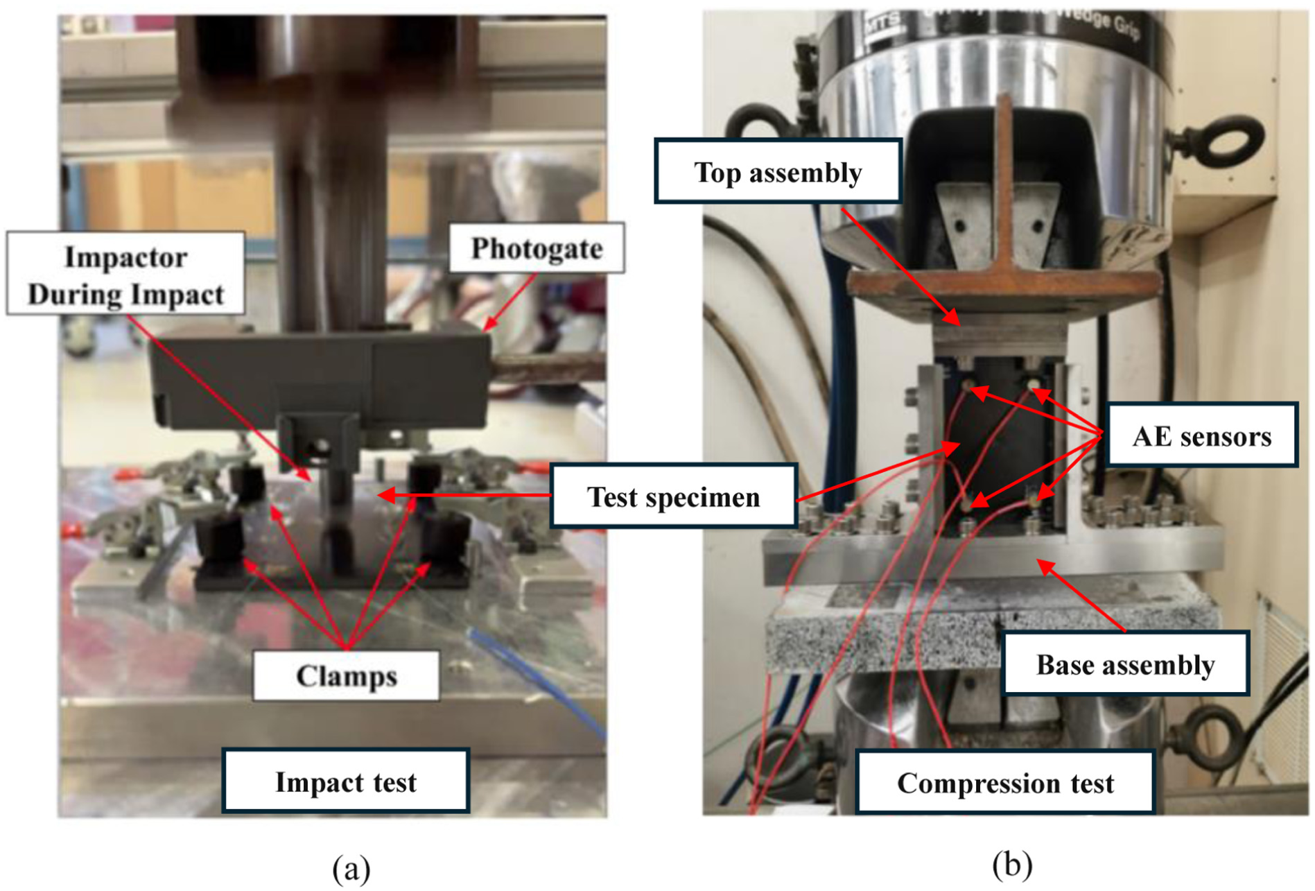
Experimental setup for the CAI test: (a) clamps securing the composite specimen and a photogate system used to measure the impact velocity and (b) the compression test fixture and sensor arrangement. CAI: compression after impact.

Figure 2 presents the frequency response plot of the Micro-30S sensor as provided by the manufacturer. The plot indicates that the sensor maintains relatively high sensitivity between approximately 100 and 600 kHz, which encompasses the primary frequency range of interest for this study (80–350 kHz). Although sensitivity diminishes below 100 kHz, the sensor remains capable of detecting signals in this lower range, making it suitable for the current application. Practical considerations also influenced the choice of the Micro-30S. Each sensor has a diameter of 10 mm, a height of 12 mm, and weighs only 6 g, making it well-suited for situations where compact size and low weight are essential, such as in-flight structural monitoring. The specimens used in this study are relatively small, and the compact form of the Micro-30S offers a better fit. Additionally, given that the broader goal of this research involves AE sensing for UAM vehicles, smaller and lighter sensors are preferred to reduce weight and simplify integration. Consequently, the Micro-30S was identified as the most appropriate sensor for this work. The AE sensor arrangement is shown in Figure 1(b), with each sensor connected to a voltage preamplifier set at a 40-dB gain. AE data were collected during the CAI testing, providing initial validation of the proposed methodology and demonstrating its potential for assessing impact damage. The CAI test setup is also depicted in Figure 1(b).

Figure 2.

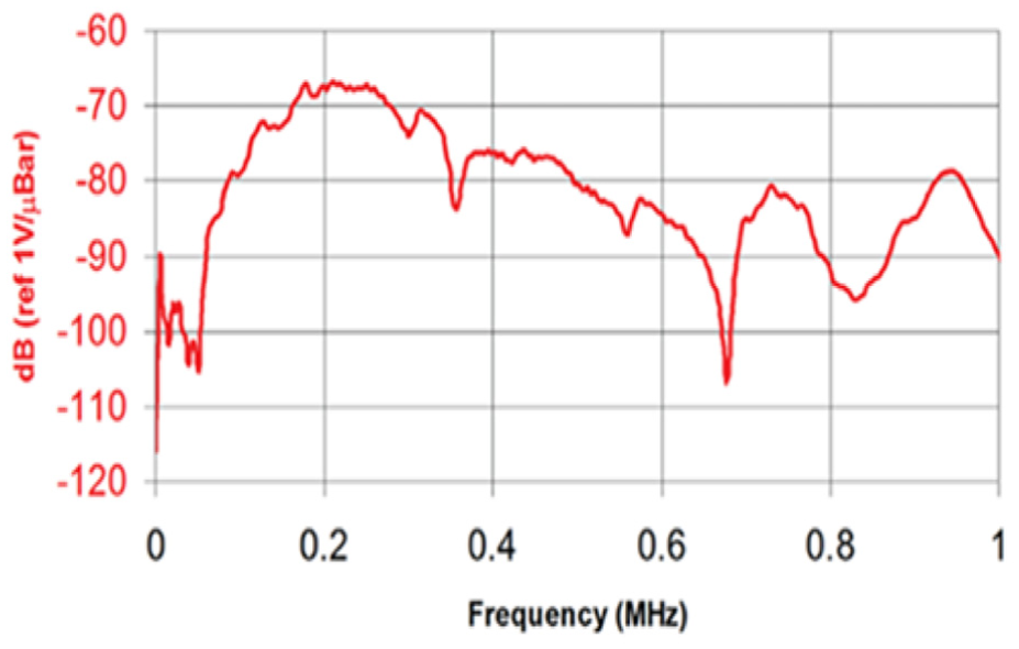
Frequency response of the Micro-30S sensor as provided by the manufacturer.

The data acquisition system was supplied by Mistras Group Inc., located in Princeton Junction, NJ. AE signals were recorded using a Digital Signal Processor system, which provides both data acquisition and analysis capabilities. Data collection was conducted with AEWin software. Signals were sampled at 1 MHz, with each AE waveform captured over a 2048 µs interval. To minimize the impact of low-amplitude background noise, a recording threshold of 40 dB was applied. The peak definition time (PDT), the interval from the first threshold crossing to the peak amplitude, was set to 200 µs, while the hit definition time (HDT), defining the end of an AE event if no further threshold crossings occur, was set to 400 µs (typically twice the PDT). AE recording commenced when the signal exceeded the threshold and ended after the HDT period, provided no additional events occurred. A hit lockout time of 400 µs was also implemented to exclude reflected or delayed signals.

Problem formulation and method of solution

The problem formulation of the work presented in this paper is explained in this section along with the method of solution. While AE signal propagation is influenced by geometric attenuation and dispersion, the proposed method emphasizes wavelet-based signal morphology associated with local damage sources. As such, scalability to large structures relies on localized sensing and appropriate sensor density, rather than global frequency invariance.

The composite specimens measured 4 × 6 inches and were prepared in accordance with ASTM 7136, making them suitable for testing small quadrotor components. However, this study primarily focused on evaluating improvements in material damage resistance rather than examining the influence of large structural dimensions on material behavior.

Implementation procedures

The stress states experienced during flight are complex and challenging to replicate precisely in laboratory environments. Accordingly, CAI tests were performed under simplified but representative conditions to evaluate the effects of impact damage on the compressive strength of composite materials. As mentioned earlier, tests involving impact energies of approximately 30 J are particularly important, as they lead to a reduction in compressive strength while the resulting damage remains barely detectable. For this reason, the current study focuses exclusively on tests performed with 30 J impact energy.

The AE technique is capable of monitoring damage evolution in composite materials under loading conditions.^51,52 Figure 3(a) illustrates a schematic of AE signal generation within composites, as captured by AE sensors. These signals can be recorded at various strain levels during a CAI test on composite specimens. Advanced approaches, including ML and deep learning models, can be employed to interpret this data and predict different modes of failure.

Figure 3.

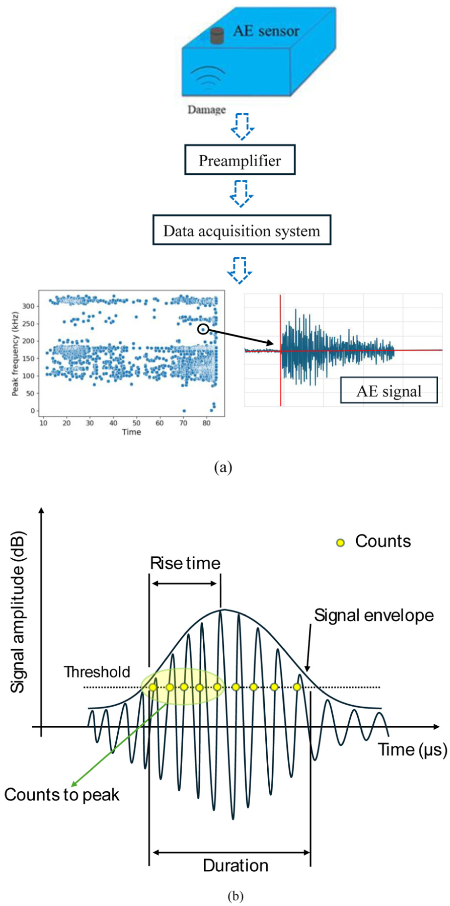
(a) AE signals produced by sensors in response to damage formation and (b) explanation of signal features.

In the AE signal processing framework, the CWT is employed to extract time–frequency features from the recorded signals and convert them into RGB wavelet images. In these images, the RGB channels represent a logarithmic transformation of the frequency content, which provides a more effective representation of the frequency range.⁴⁷ For failure mode classification, an CNN analyzes the resulting wavelet images and classifies the damage mechanisms as matrix cracking, delamination, fiber–matrix debonding, or fiber breakage.

Each AE signal is characterized by 15 distinct features, which are listed and described in Table 1, with several illustrated schematically in Figure 3(b). These features can be used as inputs to ML models such as XGBoost and random forest, as they condense the AE signals into quantitative descriptors that capture key signal characteristics. For instance, the amplitude feature corresponds to the maximum signal magnitude, count indicates the number of times the signal exceeds a predefined threshold, and rise time represents the interval between the initial threshold crossing and the signal peak.

Table 1.

Description of AE features.

AE features	Descriptions
Amplitude	The highest amplitude attained at the signal peak.
Count	The count of instances in which the signal exceeds a specified threshold.
Rise time	The time elapsed between the initial threshold crossing and the peak amplitude.
Duration	The duration between the first and last threshold crossings of the signal.
Average frequency	The mean frequency of the signal.
RMS	The RMS voltage calculated over a characteristic time window, T_RMS, ranging from 10 to 1000 ms.
ASL	The average voltage level of the signal measured over a characteristic time interval, T_ASL, ranging from 10 to 1000 ms.
Energy	The measured electrical energy associated with an AE signal.
Absolute energy	The cumulative electrical energy recorded for an AE signal.
Peak frequency	The frequency at which the signal attains its maximum amplitude.
Reverberation frequency	The frequency measured following the signal peak.
Initial frequency	The frequency measured before the signal reaches its peak amplitude.
Signal strength	A parameter that represents the intensity of the AE source.
Frequency centroid	A parameter that describes the overall frequency content of an AE signal.
Counts to peak	The total number of threshold crossings occurring between the initial crossing and the signal peak.

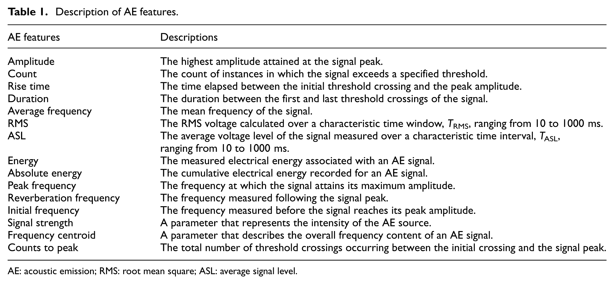
AE: acoustic emission; RMS: root mean square; ASL: average signal level.

Signal processing module

As discussed previously, the CWT is used to convert AE signals into wavelet images. CWT is a widely adopted technique for joint time–frequency analysis⁵³ and is particularly effective for identifying and emphasizing the time–frequency characteristics of non-stationary signals.⁵⁴ The CWT of a signal can be expressed as shown in Equation (1):

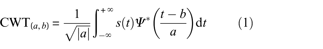
{CWT}_{(a, b)} = \frac{1}{\sqrt{| a |}} \int_{- \infty}^{+ \infty} s (t) Ψ^{*} (\frac{t - b}{a}) d t

(1)

In this context, CWT denotes the CWT coefficients obtained from the signal $s (t)$ . Parameter a represents the scale factor, which controls the dilation or compression of the wavelet, while b is the translation parameter that shifts the wavelet along the time axis. The wavelet coefficients are computed by systematically sliding wavelets of different scales across the entire signal. The symbol $Ψ^{*}$ denotes the complex conjugate of the mother wavelet ψ. In this work, the Morse wavelet⁵⁵ is selected as the mother wavelet for performing the CWT. The Fourier transform of the Morse wavelet is expressed in Equation (2).

Ψ_{p, γ} (x) = U (x) α_{p, γ} x^{\frac{p^{2}}{γ}} e^{- x^{γ}}

(2)

Here, $U (x)$ denotes the unit step function, $α_{p, γ}$ is the normalization constant, and $p^{2}$ represents the time–bandwidth product. The parameter $γ$ governs the symmetry of the Morse wavelet.⁵⁶ In this study, $p^{2}$ was set to 60 and $γ$ was set to 3.

Continuous wavelet coefficients can be visualized using scalogram images. In the proposed heterogeneous ensemble learning framework, scalograms derived from AE waveforms are used as inputs to the CNN models. All AE signals collected in this study were converted into CWT scalogram images and stored as RGB images with a resolution of 224 × 224 × 3. Scalograms generated using the Morse wavelet were compared with those obtained using two other wavelet functions, namely the analytic Morlet and Bump wavelets. The CNN models trained with Morse-based scalograms achieved slightly lower RMSE values; therefore, the Morse wavelet was selected as the mother wavelet for this study.

These continuous wavelet coefficients can be visualized in the form of a scalogram. Each AE signal recorded during the flight phase is converted into a CWT scalogram and stored as an RGB image.

Mode of failure identification module

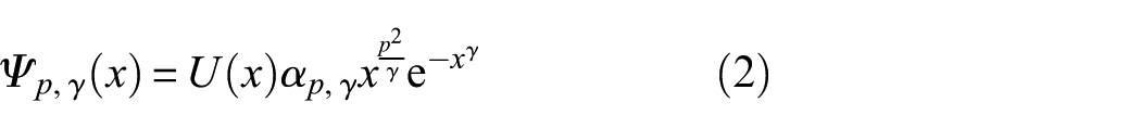
This paper introduces a heterogeneous ensemble CNN for detecting various failure modes in an impacted thermoplastic composite under compression. Such a model consists of three CNN models with distinct architectures. The ensemble is formed using the bagging aggregation technique [57]. Wavelet images serve as input to the system, with each CNN model independently analyzing the data and voting on the estimated mode of failure. The individual predictions are aggregated into a voting pool, and the final failure mode is selected based on a majority voting strategy. The overall workflow of the model is shown in Figure 4.

Figure 4.

Workflow of the proposed heterogeneous ensemble model to predict different modes of failure in a composite material.

The CNN architectures employed in the model include GoogLeNet,⁵⁸ DenseNet201,⁵⁹ and VGG-16.⁶⁰ Generally, AlexNet is a widely adopted CNN model,⁶¹ which introduced the rectified linear unit (ReLU) activation function to address the vanishing gradient issue that arises in deeper networks, replacing traditional Sigmoid and Tanh functions. It also incorporates Dropout layers to help mitigate overfitting. VGG networks were developed as an improvement over AlexNet,⁶⁰ with VGG-19 using smaller, stacked convolutional kernels instead of AlexNet’s larger ones. This design allows for deeper networks with more nonlinearities, enabling the learning of more complex features. GoogLeNet, another enhancement based on AlexNet,⁵⁸ utilizes inception modules, combinations of multiple convolutional kernels of varying sizes, rather than single convolutional layers, thereby boosting feature extraction capabilities. ResNet introduces the concept of residual learning,⁶² while DenseNet builds upon a similar principle by using densely connected convolutional blocks.⁵⁹ In DenseNet, each layer is directly connected to all subsequent layers, promoting feature reuse and enhancing the efficiency of feature extraction.

The loss function in a CNN model was cross-entropy, and the whole model was trained from scratch without freezing any layers. In all models presented in this study, the gradient descent optimization was performed using the Adaptive Moment Estimation algorithm. A minibatch size of 32, a learning rate of 0.0001, and a maximum of 30 training epochs were used.

Results and discussion

This study uses AE data collected from a CAI test performed at an impact energy of 30 J to validate the proposed methodology. The primary objective is to identify various failure modes in composite structures, especially those relevant to AAM, through deep learning techniques. The initial analysis is performed using a powerful CNN model. The effectiveness of the CNN is subsequently evaluated by comparing its performance with other ML models, such as XGBoost and random forest.

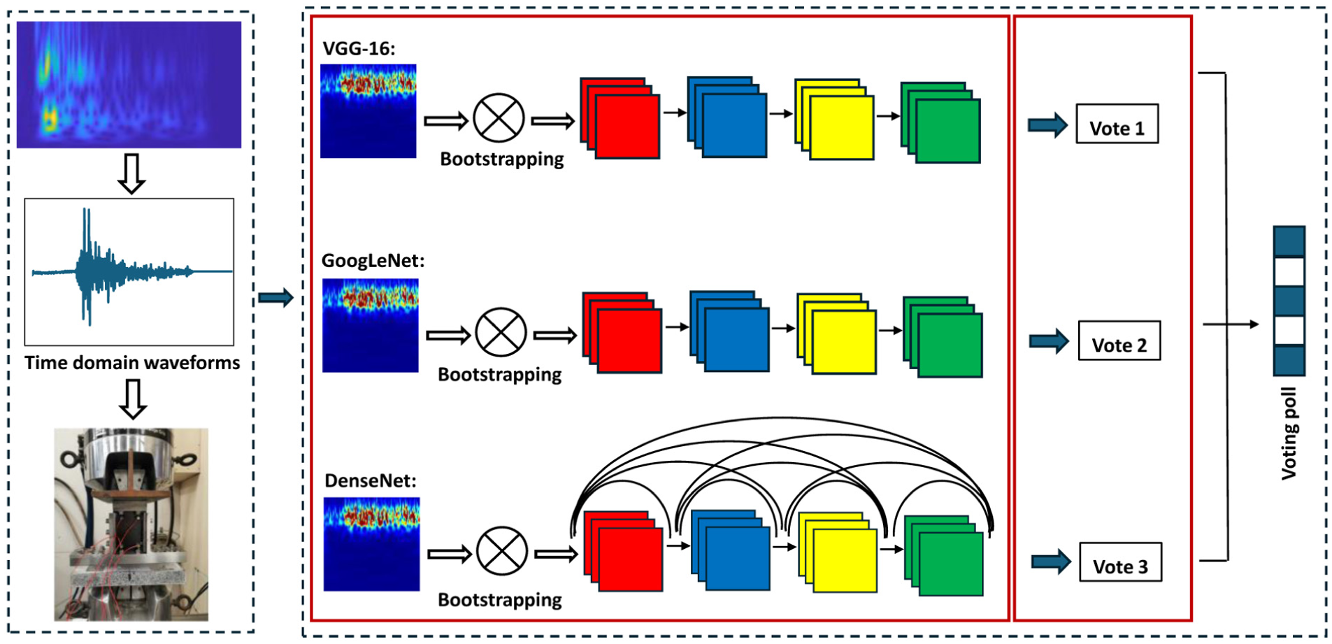
The characteristics of AE signals recorded by sensors mounted on the specimen are influenced by their peak frequencies, which correspond to different failure modes in composite materials. As such, the classification model is designed to differentiate these failure modes based on AE signals. In this study, the model input consists of AE signals represented as wavelet images, and its output is the corresponding failure mode. Figure 5 illustrates AE signals recorded during compression of an impacted specimen, categorized by peak frequency ranges. All signal amplitudes were normalized within a range of −1.0 to 1.0.

Figure 5.

AE waveforms, wavelet coefficient, and wavelet RGB images. AE: acoustic emission.

The CWT was carried out in MATLAB, which automatically determines the scale factors (a in Equation (1)) based on the signal length and the selected wavelet. For a signal length of 2048 samples and a sampling rate of 1 MHz, a total of 97 scale factors were generated, ranging from 6.8 × 10⁻⁷ to 1.7 × 10⁻⁴, with 12 voices per octave. Distinct waveform patterns corresponding to each failure mode can be observed. Figure 5 also presents the associated wavelet coefficients, with the y-axis displayed on a logarithmic scale to enhance the visibility of time–frequency components. These CWT coefficients were subsequently converted into RGB images for further analysis.

Experimental results

Composite materials are widely used in aircraft because of their high strength-to-weight ratio,⁶³ making it essential to control applied loads and understand impact damage thresholds. Damage is deemed barely visible at depths of 0.1 inches according to MIL-HDBK-17⁶⁴ under impact energies below 140 J,⁶³ which marks the limit before damage becomes easily detectable. Damage depth increases with impact energy, enhancing visibility, while low-energy impacts often produce barely visible damage that warrants careful monitoring. The CAI test was simulated using the finite element software ABAQUS by the same authors.⁶⁵ Damage progression under compressive loading was evaluated, revealing a direct relationship between compressive strength and damage severity. This relationship was also confirmed through experimental testing. Specifically, the compressive strength was observed to decrease with increasing impact energy, which can be attributed to the greater depth of damage induced by higher impact energies. A previous study by the same authors⁶⁵ showed that specimens impacted at 30 J exhibited the lowest compressive strengths despite the absence of visible damage growth, underscoring the limitations of damage assessments based solely on visual inspection. Based on these findings, the present study determines the design ultimate load (DUL) for FAR 25.305 analysis using the barely visible impact damage criterion.^63,64,66 The minimum DUL was observed for specimens impacted at 30 J, where compressive strength decreases with increasing impact energy and damage becomes progressively more visible, as illustrated in Figure 6. For impact energies below 30 J, damage remains visually undetectable while the material can still sustain additional loads. In contrast, impact energies above 30 J results in clearly visible damage accompanied by the lowest compressive strength. These results emphasize the critical importance of testing around the 30 J impact level, where damage is barely visible yet structural strength is significantly reduced.

Figure 6.

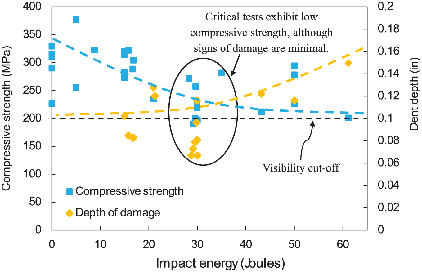
Relationship between compressive strength and damage depth for CAI tests conducted at various impact energy levels. CAI: compression after impact.

Figure 7 shows optical microscopy images of fractured specimens subjected to an impact energy of 30 J. The images were obtained using a Keyence VHX-5000 digital microscope equipped with a VH-Z20R high-performance zoom lens (Keyence Corporation of America, Itasca, IL, USA), providing magnifications from 20× to 200×. For each specimen, images captured at 100× and 200× magnification are presented, with emphasis on the fracture regions. A 500 µm scale bar is included in each image, and the composite plies have a thickness of 0.144 mm. Plies with fibers oriented at 90° are clearly indicated, while the remaining layers have fiber orientations of +45°, 0°, and −45°. Four primary failure mechanisms are identified in the 100× images and highlighted with arrows. Delamination and fiber breakage are readily observable at this magnification, whereas fiber–matrix debonding and matrix cracking are more clearly revealed at 200× magnification.

Figure 7.

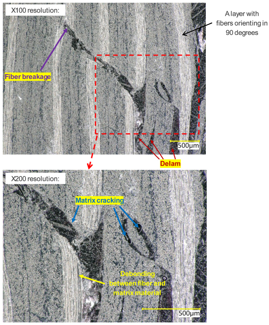
Optical microscopy images of fractured thermoplastic composite specimens illustrating various failure mechanisms at an impact energy of 30 J.

Filtering of AE signals

AE signals collected during CAI testing of similarly sized specimens often contain substantial unwanted noise resulting from wave reflections and edge effects. To enable reliable analysis, this noise must be effectively filtered. Accordingly, this study concentrates on AE signals originating from the central region of the composite panel, which is particularly prone to compressive damage.

A three-step filtering process was employed to eliminate noise. The first step involved verifying the authenticity of AE events by checking if at least three sensors detected the signal. Only events captured by a minimum of three sensors within a narrow time window of 0.0001 s were considered valid; those that did not meet this criterion were discarded. In the second step, AE source localization was carried out using an enhanced time difference of arrival (TDOA) method,⁶⁷ which is particularly effective for identifying sources in composite materials. More detailed information about this method can be found in the studies by Baxter et al.,⁶⁸ Ai et al.,⁶⁹ and Soltangharaei et al.⁷⁰ Figure 8 illustrates representative AE waveforms recorded from the composite specimen, comparing signal profiles before and after the noise filtering process. The final filtering step involved spatial filtering, in which only AE events originating from the central region of the specimen were retained. This region was defined as a 76 mm-wide band centered on the transverse midline of the plate (38 mm above and below), corresponding to the impact zone. The filtering parameters applied in this study are summarized in Table 2.

Figure 8.

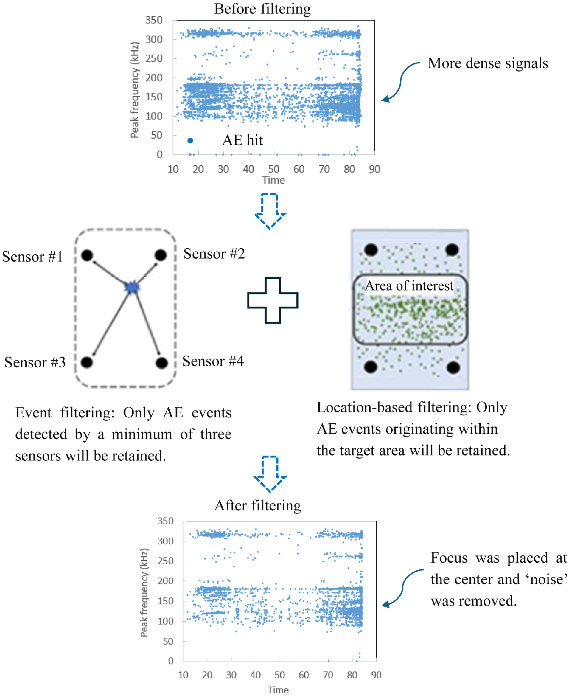
AE signals shown prior to and following the filtering process. AE: acoustic emission.

Table 2.

Parameters used in filtering process.

Parameters	Descriptions
The time interval specified in step 1.	0.0001 s
The width of the central region specified in step 3.	Transverse symmetry axis ± 38 mm

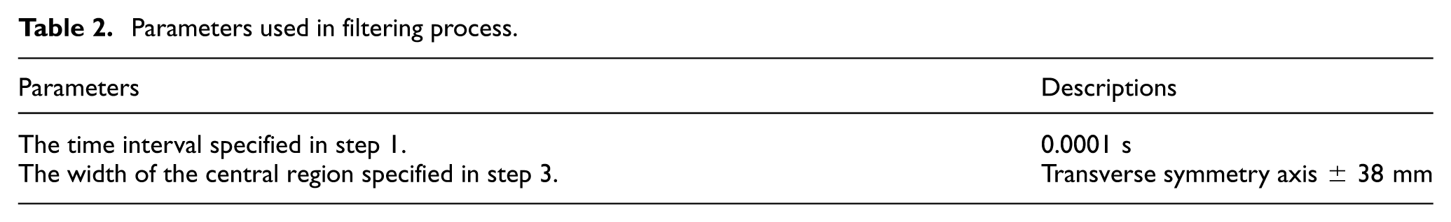
The pre-processing criteria (three sensors, 0.0001 s time threshold, TDOA, ±38 mm spatial window) were selected to optimize detection accuracy while minimizing noise. Ensuring that at least three sensors are triggered supports precise TDOA-based localization, and the time and spatial thresholds help eliminate spurious or overlapping signals. While some genuine events, such as low-amplitude signals hitting fewer sensors, events occurring in rapid succession under 0.0001 s, or those outside the ±38 mm region, may be excluded, these losses are minimal, and the remaining dataset accurately represents the overall event population.

Data preparation for AI models

Figure 9(a) displays the distribution of peak frequencies of AE signals recorded over time. Since displacements are applied progressively, the temporal distribution of data may reflect different stages of compressive strain or stress, as the applied load increases with time. As illustrated in Figure 9(a), four distinct peak frequency ranges are identified during the CAI test on thermoplastic composites impacted at 30 J. In ascending order, these frequency ranges correspond to matrix cracking, delamination, matrix–fiber debonding, and fiber breakage.

Figure 9.

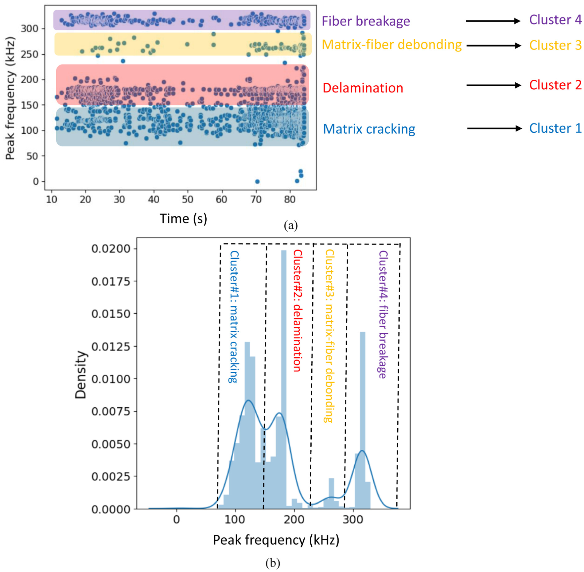
Four distinct signal states clustered based on their: (a) peak frequency and (b) temporal density.

Figure 9(b) presents the density distribution of peak frequencies over time for the same CAI test. Based on this distribution, four distinct clusters were identified, each associated with a specific failure mode, as indicated by the four prominent peaks in the frequency density curve. The associated peak frequency ranges for the different failure mechanisms are: matrix cracking (65–150 kHz), delamination (150–225 kHz), matrix–fiber debonding (225–280 kHz), and fiber breakage (280–340 kHz).

A previous study by the same author⁷¹ investigated several thermoplastic composite panels subjected to impact followed by CAI tests at impact energies ranging from 0 to 60 J. Some experiments were repeated, and the results consistently showed that the peak frequency ranges corresponding to each failure mode were similar, with comparable wavelet shapes associated with the different failure mechanisms. Based on these observations, the present study focuses on a single specimen after confirming that both the peak frequency ranges and the wavelet shapes remained consistent within specific frequency intervals.

As shown in Figure 9(b), the four clusters contain 1108, 800, 85, and 440 signals, respectively. The data distribution across the clusters reveals a noticeable imbalance. For instance, cluster 1 contains 1108 signals, whereas cluster 3 has only 85. To address this issue, several strategies have been employed, including data augmentation for cluster 3 to increase its sample size, as well as generating different data groups where clusters 1, 2, and 4 vary, but cluster 3 remains duplicated. This issue will be explored in greater detail later in the study, along with a thorough analysis of the results to identify the most effective approach for building a high-accuracy, efficient model.

Evaluation of the proposed method based on CNN model: to study the effect of imbalanced distribution of data

After converting the AE signals into RGB images, these are input into the CNN model to detect the mode of failure. In each CNN model studied, the data were then split into a training set and a test set using an 80/20 ratio. As previously noted, the data distribution across clusters is imbalanced. Initially, the model was evaluated using unbalanced data from each cluster to gauge its accuracy (see Figure 10(a)) using a homogeneous model based on only GoogleNet architecture. As illustrated in Figure 11(a), the prediction accuracy for most clusters is sufficiently high and acceptable, with the exception of cluster 3, which shows a significantly lower accuracy—47.1%, falling short of the 50.0% mark. As a result, the data from clusters 1, 2, and 4 were each divided into four distinct groups. For each of these groupings, separate models were developed—one for each group within clusters 1, 2, and 4. In this way, each of the four models contained 277, 200, 85, and 110 signals for clusters 1, 2, 3, and 4, respectively. Meanwhile, the same single group of 85 signals from cluster 3 was included in every model. The prediction accuracy for cluster 3 improved significantly, reaching 76.45%, which is considered sufficiently high. The accuracy for cluster 4 remained largely unchanged, staying above 90.0%. However, a decrease in accuracy was observed for cluster 1, while cluster 2 showed an increase. This variation can be attributed to the close proximity of frequency ranges associated with the failure modes, matrix cracking (cluster 1) and delamination (cluster 2), as illustrated in Figure 9. To further investigate the impact of data imbalance on model accuracy, the experiment was repeated using eight distinct groups for clusters 1 and 2, four groups for cluster 4, while the same dataset for cluster 3 was used across all models. In this way, each of the four models contained 138, 100, 85, and 110 signals for clusters 1, 2, 3, and 4, respectively. The accuracy for cluster 3 rose to over 90%, indicating significant improvement. Cluster 4 accuracy remained nearly the same, while the accuracies for clusters 1 and 2 declined. Once again, the accuracy for cluster 4 remained largely unchanged, likely due to the sufficient amount of data available for that cluster. The primary concern centered on the limited data for cluster 3, where a more balanced data distribution led to improved accuracy. Additionally, it should be noted that the accuracy for clusters 1 and 2 fluctuated, one increasing while the other decreased. This can be attributed to the close frequency ranges associated with these two clusters and, more importantly, to the fact that matrix cracking and delamination often occur simultaneously, as reported in the literature. As a result, the models tend to produce inconsistent accuracy levels for clusters 1 and 2.

Figure 10.

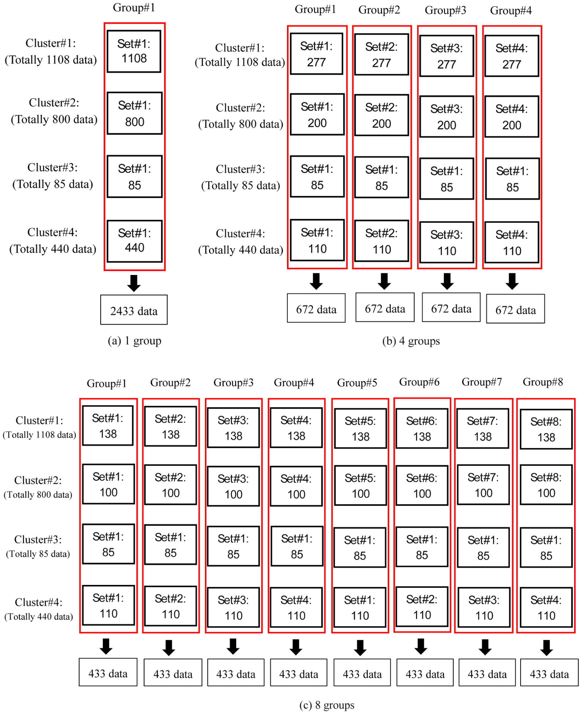
Data distribution for different numbers of groups to address the imbalance distribution of data and to understand the effect of imbalance distribution of data on model accuracy: (a) 1 group, (b) 4 groups, and (c) 8 groups.

Figure 11.

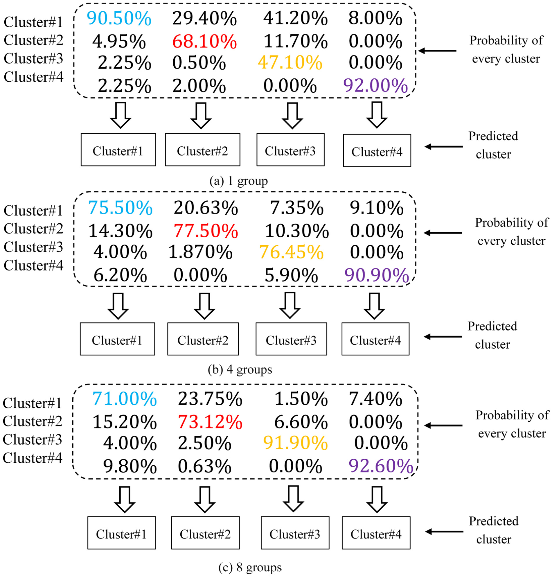
Model accuracy across various data distributions and groupings: (a) 1 group, (b) 4 groups, and (c) 8 groups.

Evaluation of the proposed method based on CNN model: to study the effect of data augmentation for cluster 3

As discussed earlier, for each CNN model evaluated, the dataset was split into training and testing sets using an 80/20 ratio. However, when constructing a heterogeneous model that combines various architectures, a portion of the data must be reserved for the voting process. This allocation reduces the available data in cluster 3, which notably impacts the accuracy of model. To address this, data augmentation was applied specifically to cluster 3 using a MATLAB function, namely additive white Gaussian noise,⁷² with a signal-to-noise ratio set at 5. This approach doubled the data for cluster 3, enabling the formation of three separate groups for clusters 1, 2, and 4. As a result, model accuracy was improved for clusters 1 and 2, particularly in cases where their frequency ranges are closely aligned. The amount of data for clusters 1 to 4 are 366, 263, 160, and 143, respectively (refer to Figure 12). It is to be emphasized that the test data were selected first, and the augmented data were subsequently added to the remaining dataset to avoid potential data leakage. Therefore, it is believed that data leakage did not occur during the modeling process.

Figure 12.

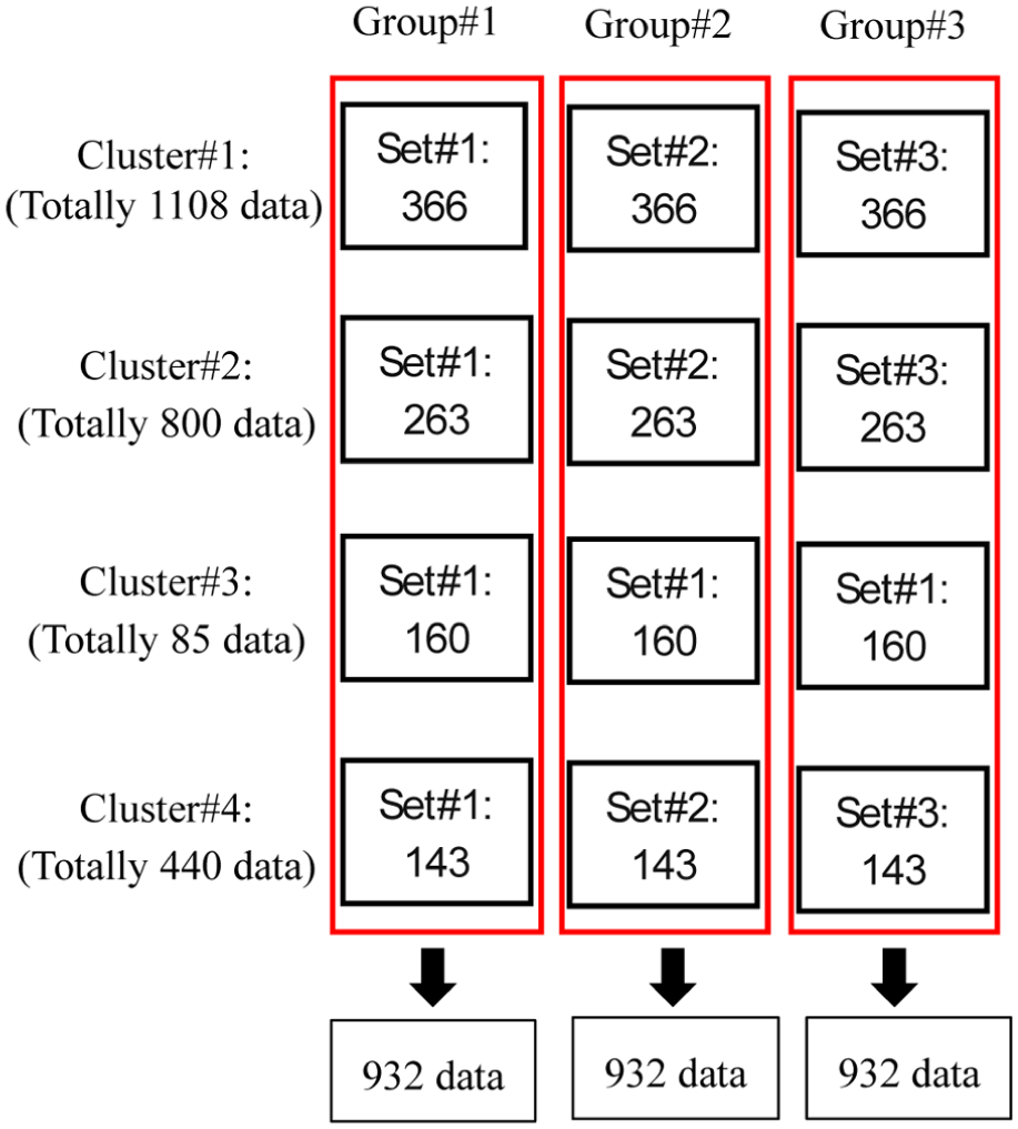
Data distribution of the augmented model after doubling the data in cluster 3, enabling the formation of three distinct clusters and improving prediction accuracy for clusters 1 and 2.

To predict various failure modes in a thermoplastic composite, three distinct architectures, GoogleNet, DenseNet201, and VGG-16, were independently employed, using the three data groups illustrated in Figure 12. Figure 13 displays the validation accuracy results for each of the three architectures. Each model demonstrates solid performance, with accuracies hovering around 80.0%. The classification results for each architecture are presented in Tables A1 to A3 in Appendix A, while Table A4 summarizes the final voting outcomes across all three models. As seen in Tables A1 through A4, the application of majority voting consistently improves prediction accuracy within each architecture as well as in the combined model. In addition, accuracy, precision, recall, and F1-score were calculated for each model and are presented in Tables A5 through A8 in the Appendix A. Confusion matrices are also provided in Figures A1 to A4 in the Appendix A.

Figure 13.

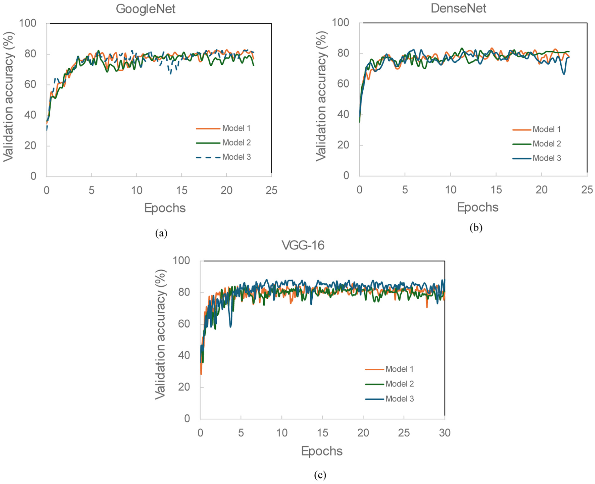
Validation curves for CNN models across three different architectures: (a) GoogleNet, (b) DenseNet, and (c) VGG-16. CNN: convolutional neural network.

As previously noted, predictions for cluster 3 are particularly challenging due to the limited amount of available data. Nevertheless, ensemble voting across the three architectures yielded accuracies of up to 50 and 60% for this cluster. Notably, the final ensemble predictions benefit when the shortcomings of one architecture are compensated by the strengths of others. For example, although VGG-16 alone achieved 50% accuracy for cluster 3, the final ensemble results improved to 70%, which is considered reasonable given the data constraints.

A similar trend was observed across the other clusters, though with generally higher accuracy levels compared to cluster 3. In the case of cluster 4, all architectures performed well, which can be attributed to the distinct separation of peak frequency values associated with fiber breakage, as shown in Figure 9. Consequently, the final voting accuracy for cluster 4 reached 100%.

While some groups within the three architectures achieved prediction accuracies of 60–70% for clusters 1 and 2, the overall accuracies for these clusters remained high, within the 90–100% range, except for cluster 1 with VGG-16, which reached 80%. As a result, the final voting accuracies for clusters 1 and 2 were 90 and 100%, respectively.

When wavelet-transformed AE signal images are input into CNN models, the convolutional layers generate high-dimensional feature representations. To visualize how these features are distributed across layers, t-distributed stochastic neighbor embedding (t-SNE) is used. This technique maps the high-dimensional data to a 2D Cartesian coordinate system, where the distances between points reflect their similarities. Figure 14 shows the feature distributions from GoogleNet, DenseNet, and VGG-16 focusing on five evenly distributed convolutional layers. In the visualization, data points are color-coded based on the corresponding damage mechanisms. In the early convolutional layer, points representing the four damage mechanisms appear widely scattered and heavily overlapped, suggesting classification challenges. As the network progresses and deeper layers extract more complex features, data points from the same category begin to cluster together, while points from different categories become more distinct. By the time the features reach the final layer, the data points form four defined clusters. However, clusters for VGG-16 exhibit more overlap compared to those for GoogleNet and DenseNet. Slight overlaps are noticeable at the cluster boundaries for GoogleNet. Overall, DenseNet presents the best distinct clusters. Figure 14 shows that the fiber breakage associated with cluster 4 is clearly separated and consistently forms its own cluster in every model. Overall, overlaps are observed among clusters 1, 2, and 3, with the most noticeable overlap occurring between clusters 2 and 3. Cluster 3.

Figure 14.

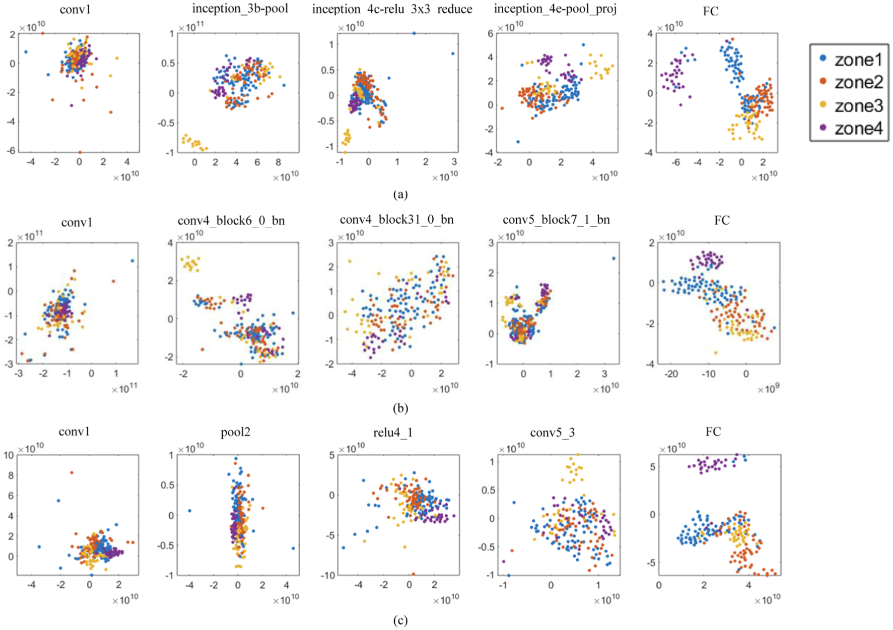
t-SNE-based visualization of feature distributions across layers for model 1 in every architecture of (a) GoogleNet, (b) DenseNet, and (c) VGG-16. t-SNE: t-distributed stochastic neighbor embedding.

As mentioned previously, damage mechanisms may occur simultaneously, especially when matrix cracking is involved. In many cases, a clear distinction between matrix cracking, delamination, and fiber–matrix debonding cannot be made. For example, matrix cracking may initiate near an interface or fiber and subsequently trigger delamination or fiber–matrix debonding, even though matrix cracking is the dominant mechanism. As a result, clustering based solely on peak frequency is insufficient to identify mixed modes of failure. A more robust approach that incorporates signal shape and wavelet characteristics is therefore required to better distinguish failure modes.

It should be noted that the effects of threshold selection on failure-mode clustering have already been assessed. The results indicate that a ±15 kHz range, or marginally wider, exerts a negligible influence on the model predictions.

The activation maps generated from both the convolutional and fully connected layers illustrate how DenseNet autonomously extracts features to identify different failure modes. These layers include Conv1, inception_3b-pool, inception_4c-relu_3x3_reduce, inception_4e-pool_proj, and the final fully connected layer. Figure 15 displays activation maps highlighting the most significant channels across several layers, capturing the fundamental patterns in the frequency distributions. As the network deepens, it learns increasingly complex features relevant to failure modes. The final fully connected layer produces a 1 × 4 vector that reflects color patterns associated with each failure mode. Notably, the vectors generated by signals from the four failure modes differ from one another. These vectors are then passed through the SoftMax layer, where they are classified according to their respective failure modes. The unique color patterns in these vectors assist in the classification process.

Figure 15.

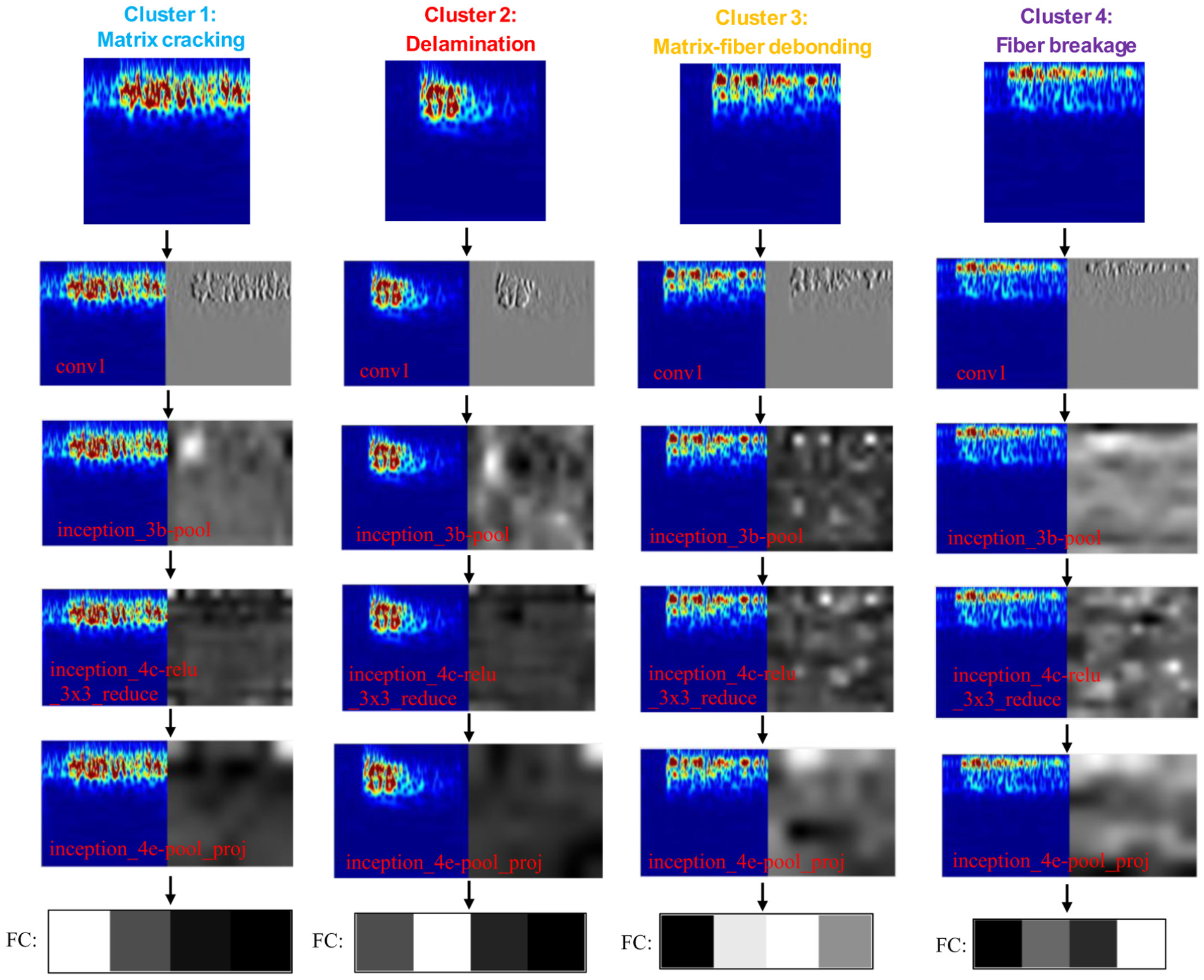
Visualization of the feature extraction process for four different modes of failure using DenseNet.

Evaluation of the proposed method based on other ML models: signal features as input

In this study, ML models like XGBoost and random forest can be used to input signal features and predict target outputs by identifying various peak frequency ranges associated with different failure modes. Figure 16(a) shows a heatmap illustrating the correlations among AE signal features during compression of the specimen impacted at 30 J. The results indicate that peak frequency exhibits a positive correlation only with the central frequency. Figure 16(b) further quantifies these correlations for the peak frequency.

Figure 16.

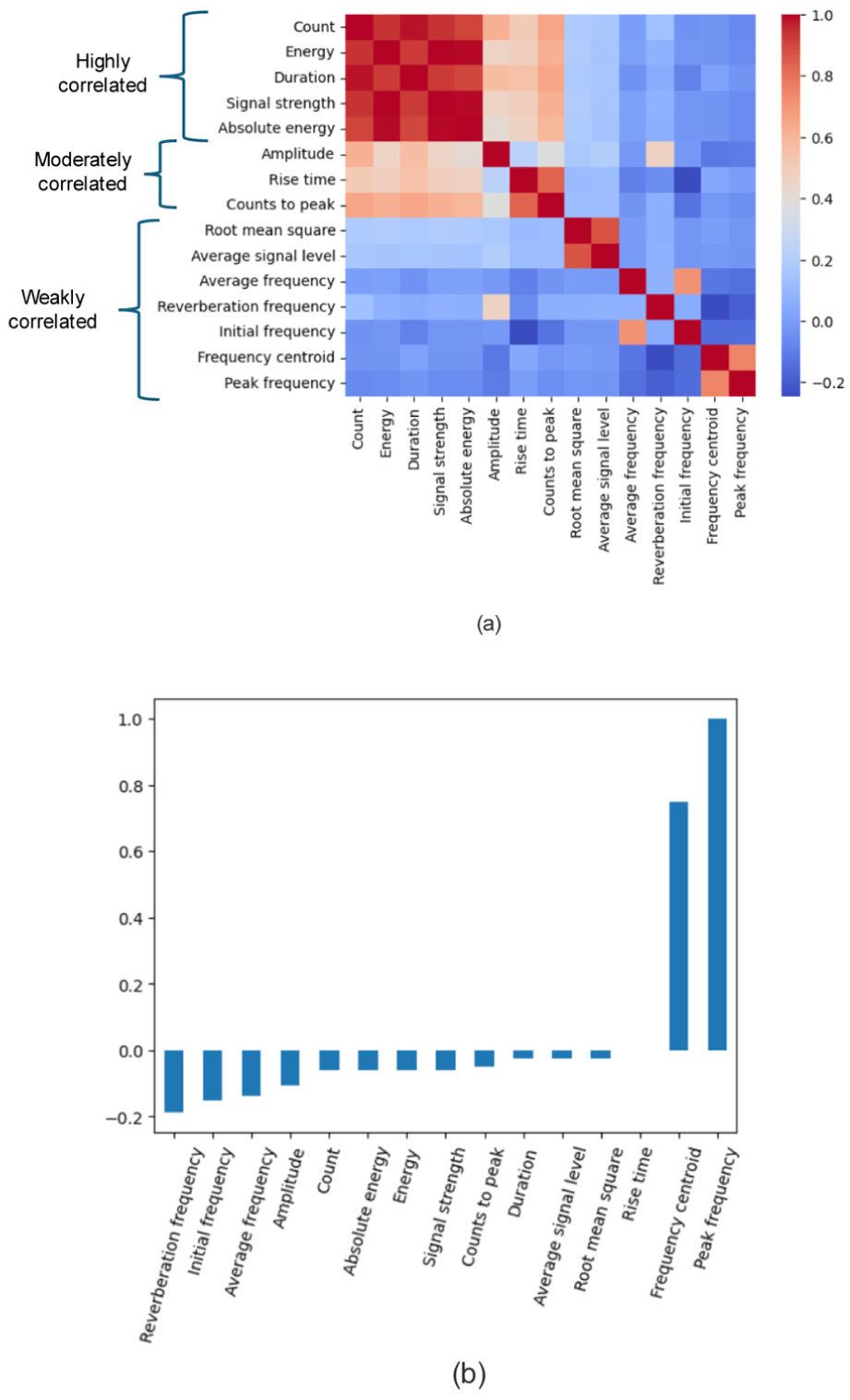
(a) Heatmap illustrating the correlations among features extracted from AE analysis during the CAI test at an impact energy of 30 J and (b) correlation values of various features with peak frequency. AE: acoustic emission; CAI: compression after impact.

As presented in Table 1, each signal contains 15 different features. These features were used as inputs to an XGBoost ML model to predict the failure mode. Since peak frequency was one of the input features and the failure modes could be distinguished based on its range, the model achieved near-perfect accuracy (refer to Figure 17(a)). To prevent this feature from dominating the prediction, peak frequency was removed from the dataset. This led to a drop in accuracy, particularly for cluster 3, which had limited data available. The prediction accuracy for cluster 3 dropped to 11.76%. In contrast, the accuracy for cluster 4 remained relatively high, while clusters 1 and 2 both achieved an accuracy of approximately 63% as shown in Figure 17(b).

Figure 17.

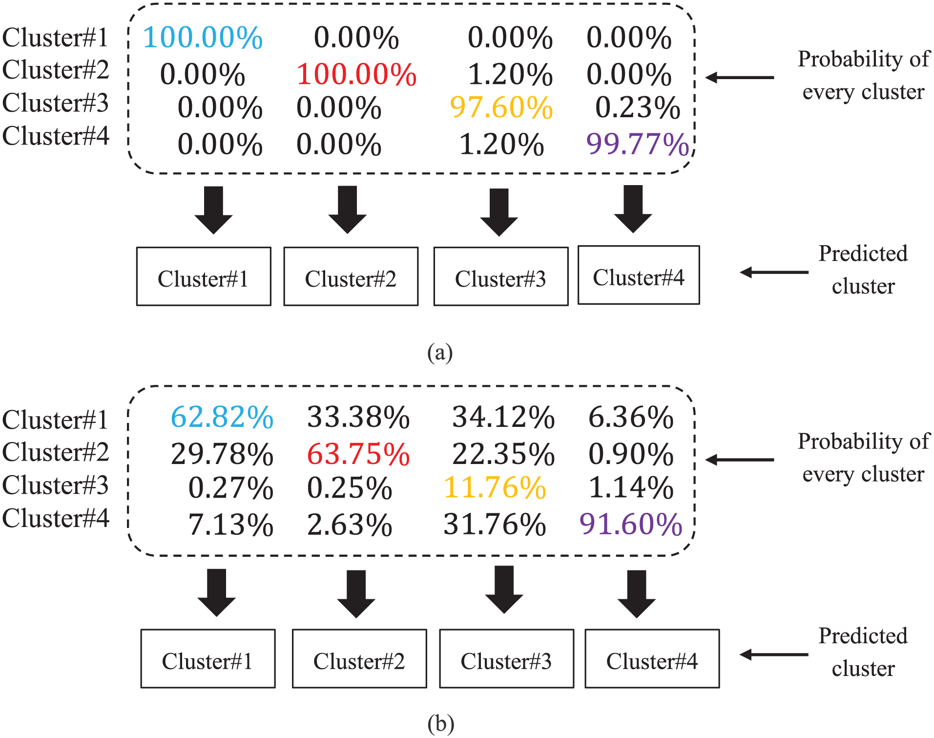
Prediction accuracy of the XGBoost model for identifying different failure modes: (a) with peak frequency included in the input dataset and (b) with peak frequency excluded.

The failure mode prediction was also carried out using the random forest model with the same input features. Similar to the XGBoost results, the model achieved nearly 100% accuracy when peak frequency was included as an input feature (refer to Figure 18(a)). When peak frequency was removed, the accuracy decreased again. Overall, the random forest model yielded results comparable to those of the XGBoost model. Notably, the prediction accuracy for cluster 3 slightly improved to 14.12% with random forest. While the accuracy for clusters 2 and 4 showed a slight decline compared to XGBoost, the accuracy for cluster 1 increased to 75.18% as shown in Figure 18(b).

Figure 18.

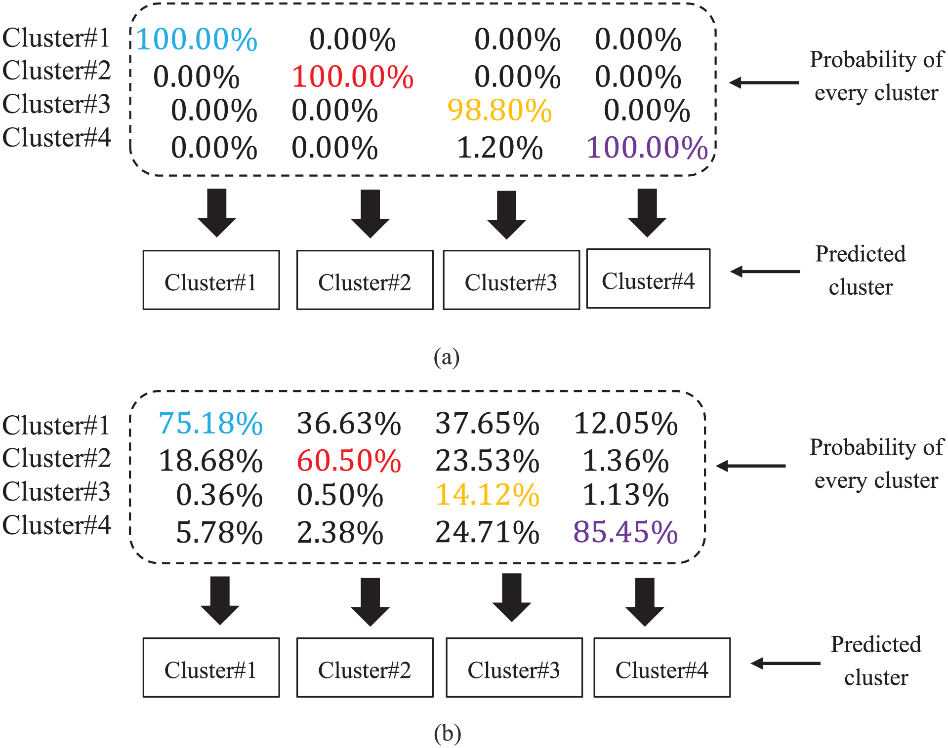
Prediction accuracy of the random forest model for identifying different failure modes: (a) with peak frequency included in the input dataset and (b) with peak frequency excluded.

Conclusions

This paper presents a methodology for identifying multiple failure modes in impacted composite components used in AAM vehicles by integrating AE sensing with deep learning techniques. The proposed approach combines AE signal analysis with CNN models to detect distinct failure mechanisms and has been experimentally validated through testing on a composite panel.

The main conclusions of this study can be summarized as follows:

The proposed method successfully identifies multiple failure modes in thermoplastic composite CAI specimens by analyzing AE signals generated under a relatively high impact energy of 30 J, which resulted in barely visible damage.

The results demonstrate that AE monitoring combined with deep learning can accurately identify multiple failure modes, highlighting its effectiveness for both potential real-time and post-impact assessments.

The heterogeneous ensemble CNN model successfully identified different failure modes—achieving prediction accuracies of 90% for matrix cracking, 100% for delamination, 70% for fiber–matrix debonding, and 100% for fiber breakage.

Two ML techniques, XGBoost and random forest, were evaluated as probabilistic classifiers using signal features as input within the proposed workflow. However, both models showed low overall prediction accuracy, particularly in detecting cluster 3.

Beyond the present findings, it is important to emphasize the key contributions of this study. The proposed approach was evaluated on a limited set of composite specimens and demonstrated strong potential for identifying multiple failure modes within a single impacted sample. To further establish the reliability and general applicability of the method, future work will focus on a more comprehensive experimental campaign involving a broader range of composite materials and operating conditions. Such efforts will enable assessment of whether the method performance can be consistently maintained across varying material behaviors and realistic application scenarios.

This study is intended as a proof-of-concept investigation demonstrating the feasibility of identifying damage mechanisms from AE signals using deep learning, rather than a statistical assessment across a large specimen population.

Footnotes

Appendix A

Table A8.

Accuracy, precision, recall, and F1-score using the heterogeneous ensemble model.

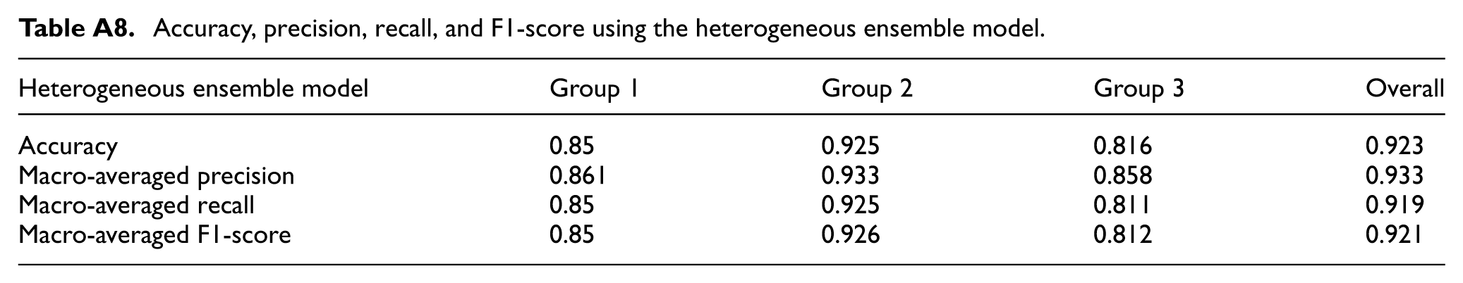
Heterogeneous ensemble model	Group 1	Group 2	Group 3	Overall
Accuracy	0.85	0.925	0.816	0.923
Macro-averaged precision	0.861	0.933	0.858	0.933
Macro-averaged recall	0.85	0.925	0.811	0.919
Macro-averaged F1-score	0.85	0.926	0.812	0.921

ORCID iDs

MM Shahzamanian

Li Ai

Paul Ziehl

Funding

The authors disclosed receipt of the following financial support for the research, authorship, and/or publication of this article: This research was conducted at the University of South Carolina and was partially funded through the NASA University Leadership Initiative Cooperative Agreement entitled Innovative Manufacturing, Operation, and Certification of Advanced Structures for Civil Vertical Lift Vehicles led by Georgia Tech, agreement number 80NSSC21M0113. The NASA technical monitor is Emilie Siochi. Opinions, interpretations, conclusions, and recommendations are those of the authors and are not necessarily endorsed by the United States Government. The project was also partially funded through the SmartState Center for Multifunctional Material and Structures.

Declaration of conflicting interests

The authors declared no potential conflicts of interest with respect to the research, authorship, and/or publication of this article.

References

Zhang

Zhou

Sun

. Bird-strike damage analysis of composite panels with different stiffeners. Aircr Eng Aerosp Technol 2022; 94(6): 933–947.

Garcia

Trendafilova

. Triboelectric sensor as a dual system for impact monitoring and prediction of the damage in composite structures. Nano Energy 2019; 60: 527–535.

Kim

D-H

Kim

S-W

. Evaluation of bird strike-induced damages of helicopter composite fuel tank assembly based on fluid-structure interaction analysis. Compos Struct 2019; 210: 676–686.

Saeedifar

Zarouchas

. Damage characterization of laminated composites using acoustic emission: a review. Compos Part B Eng 2020; 195: 108039.

Muir

Swaminathan

Almansour

, et al. Damage mechanism identification in composites via machine learning and acoustic emission. NPJ Comput Mater 2021; 7(1): 95.

Almeida

Magalhães

Karim

, et al. Identifying damage mechanisms of composites by acoustic emission and supervised machine learning. Mater Des 2023; 227: 111745.

Wang

Yan

W-J

, et al. Acoustic emission wave classification for rail crack monitoring based on synchrosqueezed wavelet transform and multi-branch convolutional neural network. Struct Health Monit 2021; 20(4): 1563–1582.

Yan

W-J

Cao

S-Z

Ren

W-X

, et al. Vectorization and distributed parallelization of Bayesian model updating based on a multivariate complex-valued probabilistic model of frequency response functions. Mech Syst Signal Process 2021; 156: 107615.

Nie

J-H

Wang

, et al. Path planning and topology-aided acoustic emission damage localization in high-strength bolt connections of bridges. Eng Struct 2025; 332: 120103.

10.

Nie

J-H

Wang

, et al. Multi-objective optimization-based acoustic emission damage location in orthotropic steel decks considering complex wave paths. Eng Struct 2025; 330: 119956.

11.

Al-Nadhari

Ulus

Topal

, et al. Analyzing stiffness variations in 3D woven composites: a multi-instrumental study on Glass/Kevlar hybridization effects under tensile and shear loads. Compos Part A Appl Sci Manuf 2025; 191: 108722.

12.

Yildirim

Ulus

Sas

, et al. Evaluating the influence of service conditions on the out-of-plane and in-plane loading performance and damage behavior of unidirectional CF/PEKK composites for aerospace applications. Compos Part B Eng 2025; 304: 112637.

13.

Senol

Ulus

Al-Nadhari

, et al. Ameliorating tensile and fracture performance of carbon fiber-epoxy composites via atmospheric plasma activation: insights into damage modes through in-situ acoustic emission inspection. Compos Part A Appl Sci Manuf 2025; 195: 108929.

14.

Nie

J-H

Wang

, et al. Acoustic emission source location in orthotropic steel decks based on topology-aided multi-objective optimization and A0 arrival time correction. Mech Syst Signal Process 2025; 230: 112614.

15.

Panasiuk

Dudzik

Hajdukiewicz

. Acoustic emission as a method for analyzing changes and detecting damage in composite materials during loading. Arch Acoust 2021; 46(3): 399–407.

16.

Nie

J-H

Wang

, et al. Damage location, quantification and characterization of steel-concrete composite beams using acoustic emission. Eng Struct 2023; 283: 115866.

17.

Pollock

. Acoustic emission inspection. Nondestruct Eval Mater 2018: 360–379.

18.

Gorman

. Plate wave acoustic emission. J Acoust Soc Am 1991; 90(1): 358–364.

19.

Suzuki

Kinjo

Hayashi

, et al. Wavelet transform of acoustic emission signals. J Acoust Emiss 1996; 14: 69–84.

20.

. Wavelet-based acoustic emission analysis of composite materials. Texas Tech University, 1996.

21.

Cui

Peng

, et al. Interface characterization of the discontinuously reinforced metal matrix composites based on wavelet analysis of acoustic emission behaviour. Chin Sci Bull 1998; 43(9): 791–792.

22.

Q-Q

Iwamoto

. Wavelet transform of acoustic emission signals in failure of model composites. Eng Fract Mech 2002; 69(6): 717–728.

23.

Barhorst

Hashemi

, et al. Discrete wavelet decomposition of acoustic emission signals from carbon-fiber-reinforced composites. Compos Sci Technol 1997; 57(4): 389–403.

24.

Ferreira

da Silva

Rebello

JMA

, et al. Failure mechanism characterisation in composite materials using spectral analysis and the wavelet transform of acoustic emission signals. Insight Non-Destr Test Cond Monit 2004; 46(5): 282–289.

25.

Kamala

Hashemi

Barhorst

. Discrete-wavelet analysis of acoustic emissions during fatigue loading of carbon fiber reinforced composites. J Reinf Plast Compos 2001; 20(3): 222–238.

26.

Boominathan

Arumugam

Santulli

, et al. Acoustic emission characterization of the temperature effect on falling weight impact damage in carbon/epoxy laminates. Compos Part B Eng 2014; 56: 591–598.

27.

Arumugam

Sidharth

AAP

Santulli

. Characterization of failure modes in compression-after impact of glass–epoxy composite laminates using acoustic emission monitoring. J Brazil Soc Mech Sci Eng 2015; 37: 1445–1455.

28.

Arumugam

Sidharth

AAP

Santulli

. Failure modes characterization of impacted carbon fibre reinforced plastics laminates under compression loading using acoustic emission. J Compos Mater 2014; 48(28): 3457–3468.

29.

Arumugam

Kumar

Santulli

. Effect of fiber orientation in unidirectional glass epoxy laminate using acoustic emission monitoring. Acta Metall Sin 2011; 24(5): 351–364.

30.

Saeedifar

Saleh

El-Dessouky , et al. Damage assessment of NCF, 2D and 3D woven composites under compression after multiple-impact using acoustic emission. Compos Part A Appl Sci Manuf 2020; 132: 105833.

31.

Ghadarah

Ayre

. A review on acoustic emission testing for structural health monitoring of polymer-based composites. Sensors 2023; 23(15): 6945.

32.

Biagini

Pascoe

J-A

Alderliesten

. Investigation of compression after impact failure in carbon fiber reinforced polymers using acoustic emission. J Compos Mater 2023; 57(10): 1819–1832.

33.

Satour

Montrésor

Bentahar

, et al. Wavelet based clustering of acoustic emission hits to characterize damage mechanisms in composites. J Nondestruct Eval 2020; 39: 1–11.

34.

Sause

Horn

. Simulation of acoustic emission in planar carbon fiber reinforced plastic specimens. J Nondestruct Eval 2010; 29: 123–142.

35.

Mao

Wang

, et al. Deep learning-based automated identification on vortex-induced vibration of long suspenders for the suspension bridge. Mech Syst Signal Process 2025; 224: 112070.

36.

Liang

Z-L

Ren

W-X

, et al. Structural damage identification under nonstationary excitations through recurrence plot and multi-label convolutional neural network. Measurement 2021; 186: 110101.

37.

Han

Liu

Wang

, et al. Multi-sensor adaptive fusion and convolutional neural network-based acoustic emission diagnosis for initial damage of the engine. Meas Sci Technol 2025; 36: 026133.

38.

Cui

Chen

, et al. Deep learning-based acoustic emission source localization in heterogeneous rock media without prior wave velocity information. Meas Sci Technol 2024; 36(1): 016011.

39.

Lin

Tang

Zhu

, et al. An acoustic emission identification model for train axle fatigue cracks based on deep belief network. Meas Sci Technol 2024; 35(7): 076125.

40.

Zhuang

Gencturk

Oberai

, et al. Impurity gas detection for SNF canisters using probabilistic deep learning and acoustic sensing. Meas Sci Technol 2024; 35(12): 126005.

41.

Shi

Deng

Yang

, et al. Research on internal leakage detection of the ball valves based on stacking ensemble learning. Meas Sci Technol 2024; 35(9): 095109.

42.

Nie

Wang

, et al. Loading condition monitoring of high-strength bolt connections based on physics-guided deep learning of acoustic emission data. Mech Syst Signal Process 2024; 206: 110908.

43.

Chen

Wang

, et al. Deep learning-based acoustic emission data clustering for crack evaluation of welded joints in field bridges. Autom Constr 2024; 165: 105540.

44.

Shevchik

Kenel

Leinenbach

, et al. Acoustic emission for in situ quality monitoring in additive manufacturing using spectral convolutional neural networks. Addit Manuf 2018; 21: 598–604.

45.

Hesser

Mostafavi

Kocur

, et al. Identification of acoustic emission sources for structural health monitoring applications based on convolutional neural networks and deep transfer learning. Neurocomputing 2021; 453: 1–12.

46.

Lee

Bak

, et al. Damage localization using acoustic emission sensors via convolutional neural network and continuous wavelet transform. Mech Syst Signal Process 2023; 204: 110831.

47.

Bayat

Ziehl

. Localizing damage on stainless steel structures using acoustic emission signals and weighted ensemble regression-based convolutional neural network. Measurement 2023; 211: 112659.

48.

Karthik

Kumar

. A comprehensive review on damage characterization in polymer composite laminates using acoustic emission monitoring. Russ J Nondestruct Test 2022; 58(8): 705–721.

49.

Qing

Liao

Wang

, et al. Machine learning based quantitative damage monitoring of composite structure. Int J Smart Nano Mater 2022; 13(2): 167–202.

50.

ASTM D7137. Standard test method for compressive residual strength properties of damaged polymer matrix composite plates.

51.

Soltangharaei

Bayat

, et al. Detection of impact on aircraft composite structure using machine learning techniques. Meas Sci Technol 2021; 32(8): 084013.

52.

Mesaric

Flowers

, et al. Evaluation of impact energy in composites using acoustic emission sensing technique. Meas Sci Technol 2024; 36(1): 0161a4.

53.

Zhou

. Empirical Fourier decomposition: an accurate signal decomposition method for nonlinear and non-stationary time series analysis. Mech Syst Signal Process 2022; 163: 108155.

54.

Shi

Cao

Wang

, et al. A directional continuous wavelet transform of mode shape for line-type damage detection in plate-type structures. Mech Syst Signal Process 2022; 167: 108510.

55.

Lilly

Olhede

. Generalized Morse wavelets as a superfamily of analytic wavelets. IEEE Trans Signal Process 2012; 60(11): 6036–6041.

56.

Lilly

Olhede

. Higher-order properties of analytic wavelets. IEEE Trans Signal Process 2008; 57(1): 146–160.

57.

Oza

Russell

. Online bagging and boosting. In: International workshop on artificial intelligence and statistics, 2001, pp. 229–236. PMLR.

58.

Szegedy

Liu

Jia

, et al. Going deeper with convolutions. In: Proceedings of the IEEE conference on computer vision and pattern recognition, Boston, MA, USA, 8–10 June 2015.

59.

Huang

Liu

van der Maaten

, et al. Densely connected convolutional networks. In: Proceedings of the IEEE conference on computer vision and pattern recognition, Honolulu, Hawaii, 21–26 July 2017, pp. 770–778. IEEE.

60.

Simonyan

Zisserman

. Very deep convolutional networks for large-scale image recognition. arXiv preprint arXiv:1409.1556, 2014.

61.

Iandola

Han

Moskewicz

, et al. SqueezeNet: AlexNet-level accuracy with 50x fewer parameters and< 0.5 MB model size. arXiv preprint arXiv:1602.07360, 2016.

62.

Zhang

Ren

, et al. Deep residual learning for image recognition. In: Proceedings of the IEEE conference on computer vision and pattern recognition, Las Vegas, NV, USA, 26 June–1 July 2016. IEEE.

63.

Cook

. Visual inspection reliability for composite aircraft structures. 2009.

64.

MIL-HDBK-17/3F. Composite materials handbook: polymer matrix composites materials usage, design, and analysis, 2002.

65.

Shahzamanian

Houck

, et al. Experimental and simulation of compression after impact (CAI) tests for thermoplastic composite materials. Appl Compos Mater 2025: 1–36.

66.

Esp

. Practical analysis of aircraft composites. Atlanta, GA: Grand Oak Publishing, 2017.

67.

Chestnut

. Emitter location accuracy using TDOA and differential Doppler. IEEE Trans Aerosp Electron Syst 1982; 18(2): 214–218.

68.

Baxter

Pullin

Holford

, et al. Delta T source location for acoustic emission. Mech Syst Signal Process 2007; 21(3): 1512–1520.

69.

Soltangharaei

Greer

, et al. Structural health monitoring of stainless-steel nuclear fuel storage canister using acoustic emission. Dev Built Environ 2024; 17: 100294.

70.

Soltangharaei

Hill

, et al. Acoustic emission technique to identify stress corrosion cracking damage. Struct Eng Mech 2020; 75(6): 723–736.

71.

Shahzamanian

Houck

, et al. Acoustic emission data analysis of compression after impact tests for composite materials. J Nondestruct Eval 2025; 44(4): 153.

72.

Iqbal

Khan

Naveed

, et al. Recent trends and advances in fundus image analysis: a review. Comput Biol Med 2022; 151: 106277.

AI-driven detection of failure modes in thermoplastic composites using acoustic emission techniques

Abstract

Keywords

Introduction

CAI experiment

Problem formulation and method of solution

Implementation procedures

Signal processing module

Mode of failure identification module

Results and discussion

Experimental results

Filtering of AE signals

Data preparation for AI models

Evaluation of the proposed method based on CNN model: to study the effect of imbalanced distribution of data

Evaluation of the proposed method based on CNN model: to study the effect of data augmentation for cluster 3

Evaluation of the proposed method based on other ML models: signal features as input

Conclusions

Footnotes

Appendix A

ORCID iDs

Funding

Declaration of conflicting interests

References