Sage Journals: Discover world-class research

Abstract

The monitoring of large-scale civil infrastructure, such as railways and tunnels, using distributed sensing systems, for example, fiber-optic sensing, is cost-effective and hence highly promising. However, compared to conventional spot sensors, distributed sensing systems still face some challenges, for example, measurement accuracy and physical interpretability. In this study, we employ a distributed acoustic sensing (DAS) system to detect rail fastener failures and propose an interpretable cross-modal transfer learning approach to address these challenges. This method enables the fusion of acceleration and DAS signals within a deep learning framework, leveraging interpretability techniques to infer the rationale behind model predictions. Additionally, a field test focusing on rail fastener failures was conducted, during which the dynamic responses of the rail under various fastener failure conditions were independently measured using accelerometers and DAS. The proposed method was applied and validated using field test data. Results demonstrate that the deep learning model trained with the proposed cross-modal transfer learning method achieves superior accuracy compared to traditional methods using DAS data alone. Furthermore, interpretable features were successfully extracted in the proposed model for follow-up predictions, underscoring its enhanced generalization capability and interpretability for rail track monitoring. These results highlight not only the method’s effectiveness for rail monitoring but also its potential applicability to other civil structures requiring integrated distributed and point sensing.

Keywords

Rail track monitoring fastener failure detection distributed sensing deep learning transfer learning

Introduction

Railway infrastructure, for example, railway tracks, is critical for modern societal and economic development, owing to its efficiency, safety, and environmental friendliness. However, railway infrastructure gradually deteriorates due to prolonged usages and external environmental factors.^1,2 Simultaneously, the intensification of climate change, such as extreme storms and floodings, poses new challenges to the structural integrity and safety of railway tracks.^3–6 Accordingly, ensuring the health and safety of railway tracks has become increasingly vital. Conventional track monitoring methods primarily depend on manual inspections, which are both labor-intensive and costly. The adoption of advanced technologies and intelligent maintenance solutions for automated real-time track monitoring is an unmet need for both industrial and academia communities of railway engineering.^7–10 In particular, the failure of rail fasteners is considered one of the most common faults in railway infrastructure during operations, typically manifested as fastener loosening or breakage.^11,12 When a fastener fails, it provides insufficient downward pressure on the rail, compromising the rail position and stability. Such abnormalities not only accelerate the wear of other components within the track system but also affect train operational smoothness, increasing maintenance costs and safety risks.^13–15 More critically, in extreme cases, fastener failure can result in severe rail displacement or even fracture, potentially leading to derailments and other major operational accidents.^16,17 Therefore, monitoring and maintaining the condition of rail fasteners is of paramount importance for ensuring the safe operation of railway systems.

In recent years, various efforts are made to address the challenges, with several sensing and detection technologies being extensively explored for monitoring fastening failures. Among these, image processing technologies have attracted significant attention.^18–20 For instance, Bai et al.²¹ developed a convolutional neural network (CNN) model trained on image data of fasteners under diverse conditions, enabling the deep learning model to effectively identify fastening failures. However, despite the promising results in controlled environments, image-based technologies face several challenges in practical engineering applications.²² External factors, such as variations in weather conditions, fluctuations in lighting intensity, surface contamination of the ballast, and dynamic interference caused by high-speed train operations, can adversely affect image quality.^23,24 These factors may significantly reduce the accuracy of deep learning models in real-world scenarios, posing substantial limitations to their deployment in railway monitoring systems.

In addition, several researchers have also studied detection of fastener failure based on vibration responses, with its primary advantage lying in the direct detection of changes in the mechanical properties of the rail.^25,26 However, current studies are largely focused on laboratory experimental settings, for instance, Wang et al.²⁷ analyzed vibration response variations in fasteners under different conditions through hammering tests, highlighting changes linked to fastener failure. While accelerometers offer high precision in vibration detection, their single-point measurement capability limits their applicability to real-world railway networks, particularly those extending over hundreds of kilometers. In recent years, various distributed sensing systems have been proposed for structural health monitoring.^28–30 These systems operate based on the propagation characteristics of laser light within optical fibers, enabling the monitoring of environmental factors along the fiber path, for example, the distributed acoustic sensing (DAS) system can detect acoustic and vibration signals through distributed fiber-optic sensors.^31–33 This makes the application of DAS technology in long-distance railway track health monitoring a promising concept. However, signals obtained from DAS systems often exhibit limited physical interpretability and high complexity, posing significant challenges in extracting meaningful information about structural health conditions.^34–36 Although advanced deep learning methods can be used for training and prediction on these data, the internal mechanisms of these models are opaque, and their prediction results often lack sufficient interpretability, which limits their widespread adoption in engineering fields.³⁷

To address the constraints or issues of the current monitoring technologies, this study aims to apply DAS technology to the health monitoring of railway and proposes a rail fastener failure detection method based on an interpretable deep learning model. The method utilizes DAS technology and optimizes the deep learning model by integrating the rail acceleration signals, thereby enhancing its generalization ability. Specifically, a cross-modal transfer learning approach is proposed, which extracts the mechanical characteristic information of the rail embedded in the acceleration data and applies such knowledge into the deep learning model based on distributed sensing, achieving effective fusion of multimodal data. In addition, an interpretable deep learning framework is developed to provide detailed explanations of the model’s detection knowledge basis. Finally, field experiments are conducted to validate the effectiveness and feasibility of the proposed method.

The rest of the article is organized as follows: the second section provides a detailed description of the research methodology, including the mechanical principles, the proposed deep learning approach, and the corresponding interpretability techniques. The third section presents a field experiment on rail fastener failures and corresponding results. The fourth section demonstrates the performance of the proposed method on experimental field data, including the accuracy of model detection and the rationale behind model predictions derived from interpretability techniques. Finally, the fifth section concludes the research and presents an outlook for future work.

Methodology

In this section, the mechanical basis for detecting the failure of rail fastener clips is introduced in “Mechanical foundation for rail fastener clip failure detection” section. “Deep learning network architecture” section presents the deep learning model used in this study, including its overall structure and details of each module. “Cross-modal transfer learning” section describes the proposed cross-modal transfer learning method, covering the model training process, the composition of the loss function, and its working principles. Finally, “Interpretable mechanisms” section introduces the principles and implementation process of the interpretability techniques used in this study.

Mechanical foundation for rail fastener clip failure detection

Figure 1 illustrates the fastening system and its mechanical model. From Figure 1(a), it can be observed that a typical fastening system mainly consists of the clips, screw spikes, and pads. Among these, the fastening pads provide elastic support for the rail, while the screw spikes secure the baseplate and the pad firmly to the sleeper. The fastening clip applies downward pressure on the rail, ensuring close contact between the rail and the fastening pad. Two mechanical models³⁸ for the fastening system are shown in Figure 1(b) and (c). In the solid-contact model, the fastening pad is modeled as an elastic solid, while the mechanical effect of the fastening clip on the rail is represented by a spring-damper element in this model. Additionally, the spring-damper model is a more simplified approach and the most commonly used model in track dynamic analysis. It is widely applied in engineering practices such as track design and modeling. In this model, the effects of the clip and pad are integrated and simplified into a spring-damper element, where the elastic support provided to the rail is governed by the stiffness k.

Figure 1.

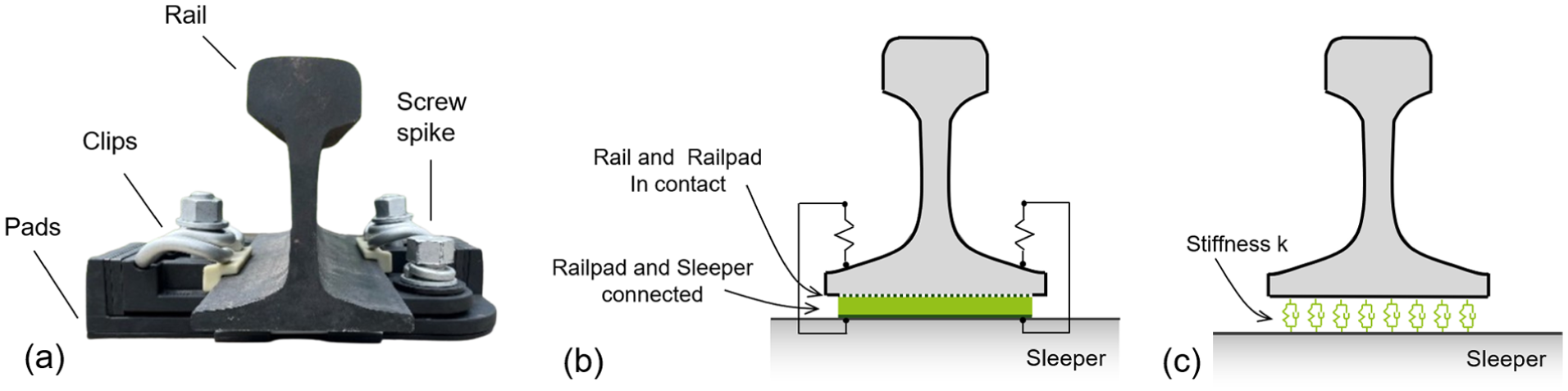
Fastening system and its mechanical model schematic diagrams: (a) typical fastening system, (b) solid-contact model for the fastening system, and (c) spring-damper model for the fastening system.

It can be found that the primary role of the fastening clip in the mechanical system is to ensure close contact between the rail and the fastening system, while its dynamic characteristics are not significant in track dynamic analysis. However, when the fastening clip becomes loose, the contact relationship between the rail and the pad transitions to partial contact or even no contact. This can be represented in the spring-damper model as a reduction in the spring stiffness k, which further leads to decreases in the natural frequency of the rail system, such changes can be reflected in the free vibration response of the rail. Moreover, if the number of loose fasteners near a section of rail increases, the natural frequency of the rail will change further. Therefore, this study aims to detect loose fasteners in the rail system by monitoring the free vibration response of the rail after dynamic excitation.

DAS is an advanced sensing technology based on optical fiber, which is able to measure external vibrations by analyzing the phase change of backscattered light in the optical fiber.³⁹ The basic principle is to use optical fiber as the sensing medium, when the rail produces vibration, these vibrations will cause small local deformation of the optical fiber, which will lead to changes in the phase of the scattered light in the optical fiber. By demodulating the phase change, the DAS system can obtain the vibration response signal of the rail.^40,41 Therefore, this article proposes to utilize the DAS system to measure the response of free vibration of rails in different conditions of fasteners, and then achieve the detection of the failure of rail fasteners. Specifically, a fastener failure index (FFI) is defined in this study, representing the number of loose fasteners within a certain range of the rail. When this index is 0, it indicates that all fasteners on the rail are securely tightened.

Deep learning network architecture

The proposed deep learning model aims to predict the rail FFI based on the measured vibration response of the rail. Since the FFI is treated as a continuous variable, the task is formulated as a regression problem to support model interpretability. This formulation enables the use of interpretation techniques such as LIME to identify which parts of the input signal contribute positively or negatively to the predicted FFI, offering deeper insights into the model’s decision-making process. The architecture of the deep learning network model proposed in this study is shown in Figure 2. It consists of a signal input layer, CNN blocks, transformer blocks, and an output layer. Specifically, the signal input layer can accept multichannel signals, such as multidirectional acceleration signals or DAS signals from multiple sensing points (SPs). Since this study uses the free vibration response of the rail to detect fastener failure, and the amplitude of the time-domain response typically varies with the excitation source, the frequency spectrum sequence of the free vibration response is considered more suitable as the model input.

Figure 2.

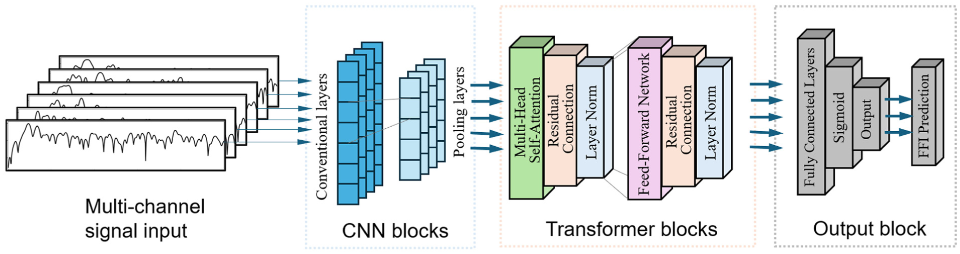
The framework of the deep learning model used for identifying fastener failure.

The CNN architecture has been widely adopted in various signal processing and pattern recognition tasks due to its effectiveness in hierarchical feature extraction.^42–44 In this research, the CNN blocks are used to reduce the dimensionality and compress the input raw signals, extracting key features from the signals to alleviate the computational complexity of subsequent network layers. The CNN blocks mainly consist of convolutional layers and pooling layers, which can be computed as follows^45,46:

y_{n} = f (c k_{n} \otimes Y + b_{n}), n = 1, \dots, N

(1)

{\bar{y}}_{n} = max {y_{n}}

(2)

where $y_{n}$ represents the nth feature extracted in the convolutional layer, $c k_{n}$ denotes the nth convolution kernel, $b_{n}$ is the nth bias, and $Y$ is the input signal fed into the convolutional layer. $N$ represents the total number of convolution kernels in the layer, $\otimes$ denotes the convolution operation, and $f (\cdot)$ is the nonlinear activation function, and ${\bar{y}}_{n}$ denotes the feature with reduced size in the pooling layer.

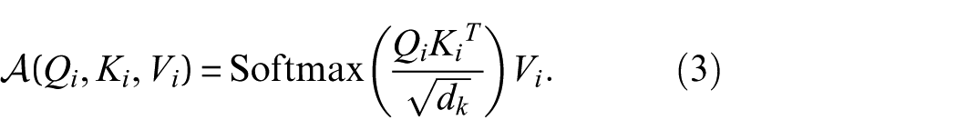
The transformer blocks are used to capture the global dependencies of the signal. By leveraging the self-attention mechanism, it can dynamically assign weights to different sections of the signal. Originally introduced for sequence modeling in natural language processing, the transformer architecture has since demonstrated strong capability in learning long-range relationships across various domains.^47–49 Specifically, each transformer module consists of a multihead self-attention layer and a fully connected feed-forward layer.^50–52 Each layer is followed by a residual connection and a normalization layer. The input to the attention function consists of queries and keys with dimensions d_k and values with dimension d_v. To enable parallel computation, a set of queries and keys is packed into matrices Q and K, respectively. The corresponding values are also packed into matrix V. Then, the attention function A is computed as follows:

A (Q_{i}, K_{i}, V_{i}) = Softmax (\frac{Q_{i} {K_{i}}^{T}}{\sqrt{d_{k}}}) V_{i} .

(3)

The multihead attention mechanism splits the attention into h heads, with each head calculated independently. After computing the attention for each head, their outputs are concatenated and passed through a final linear transformation to obtain the output. The multihead attention function M is defined as follows:

M (Q, K, V) = Concat (A_{1}, \dots, A_{h}) W^{O}

(4)

where $W^{O}$ is a projected parameter matrix used to remap the result of concatenation to output dimensions of the block.

After the feature extraction of the raw signals by the CNN and transformer blocks in the encoder, a fully connected layer is used for information integration and to output the prediction result, which is the FFI.

Cross-modal transfer learning

Since the DAS system enables distributed monitoring, it is more suitable for fastener failure detection on railway tracks spanning tens of kilometers. However, its vibration monitoring primarily relies on the Rayleigh scattering effect, using the slight phase shift caused by vibration in the optical fiber to detect vibrations along the fiber. As a result, compared to traditional vibration measurement devices such as accelerometers, the data from DAS typically contains more noise and may be more difficult to interpret. Therefore, a promising approach is to transfer the features measured by the accelerometers into the DAS data, enabling monitoring based on DAS.

In traditional transfer learning tasks, knowledge is usually transferred between different domains with the same type of data.^53,54 However, in this study, we aim to transfer the key features of rail vibration obtained from accelerometer signals into a network that uses DAS signals as input. The data acquisition methods for DAS signals and accelerometer signals are completely different, which means that the deep learning network extracts features from these two types of signals in fundamentally different ways. Therefore, cross-modal transfer learning is proposed in this study. It is important to note that in machine learning-related research, the term of data modal typically refers to different types of data forms, which is not the same concept as modalities in structural dynamics. The cross-modal transfer-learning framework proposed in this article is shown in Figure 3.

Figure 3.

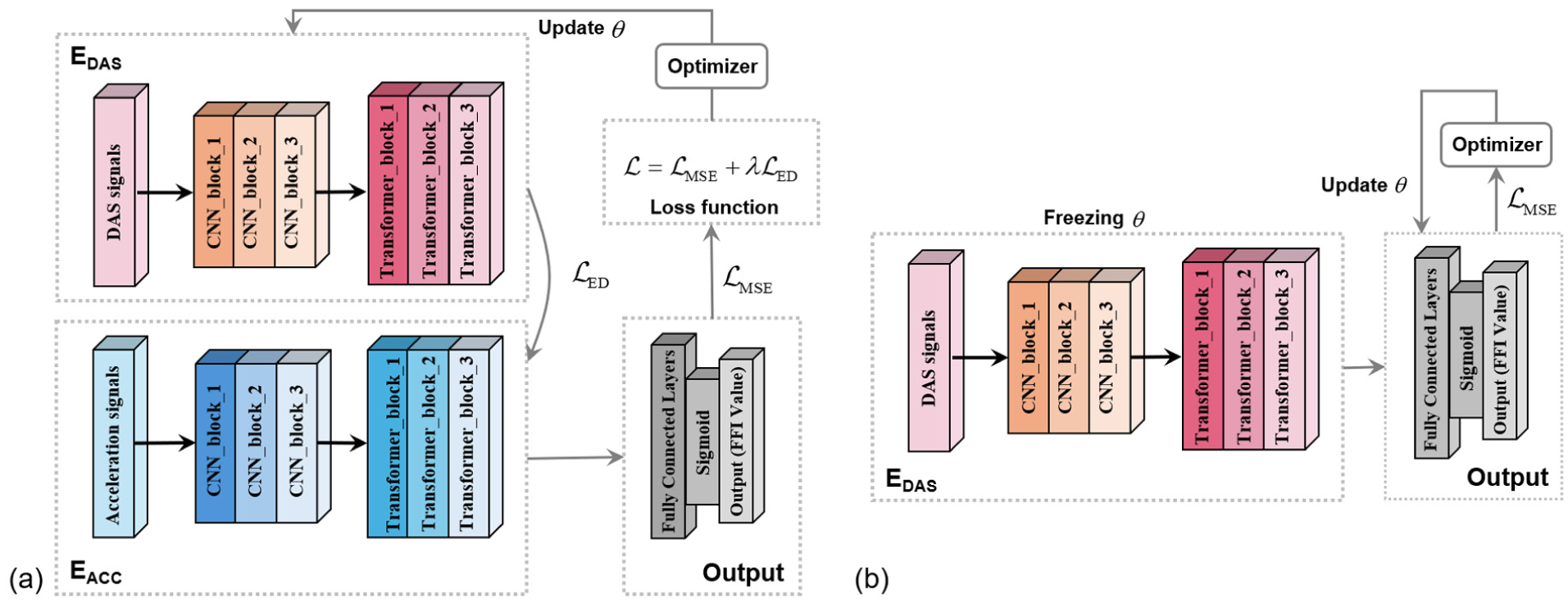
The deep learning training process of the proposed cross-domain adaptation: (a) pretraining the model using multiple data sources and (b) fine-tuning the model on the target domain.

In our framework, two independent encoders, $E_{ACC}$ and $E_{DAS}$ , are designed to extract features from accelerometer and DAS signals, respectively. During the pretraining phase, both types of signals are fed into their corresponding encoders. The accelerometer branch contributes directly to the output prediction, while the DAS branch is trained to align its feature distribution with that of the accelerometer branch. This alignment is enforced by a composite loss function composed of three terms. The first term is the mean squared error (MSE) loss, defined as follows:

L_{MSE} = \frac{1}{n} \sum_{i = 1}^{n} {(y_{i} - {\hat{y}}_{i})}^{2}

(5)

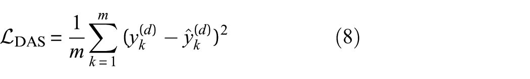
where n represents the number of samples, ${\hat{y}}_{i}$ represents the model’s predicted values, and $y_{i}$ represents the true values.

The second term is encoder discrepancy (ED) loss $L_{ED}$ , which is defined as follows:

L_{ED} = ‖ E_{ACC} (x) - E_{DAS} (x) ‖^{2}

(6)

which minimizes the direct $ℓ_{2}$ difference between the outputs of the two encoders. By combining the two terms, the model not only ensures accurate predictions on the accelerometer side but also encourages the DAS encoder to learn features with a distribution closely aligned to that of the accelerometer encoder, thus reducing the domain gap between the two modalities.

The overall pretraining loss is a weighted sum of these terms:

L = L_{MSE} + λ L_{ED}

(7)

with hyperparameter $λ$ balancing the contributions of the ED and MSE losses.

As shown in Figure 3(b), after pretraining, the weights of $E_{DAS}$ are frozen, and the accelerometer branch is removed. The DAS encoder is then fine-tuned with a new output layer using DAS signals alone. The fine-tuning loss is defined as follows:

L_{DAS} = \frac{1}{m} \sum_{k = 1}^{m} (y_{k}^{(d)} - {\hat{y}}_{k}^{(d)})^{2}

(8)

where $m$ is the number of DAS samples, and ${\hat{y}}_{k}^{(d)}$ is the prediction produced by the frozen DAS encoder and the new output layer. This enables the network to be retrained for fastener failure detection using DAS signals.

Interpretable mechanisms

Typically, deep learning models are considered black boxes, meaning that their decision-making processes are often difficult to interpret.^55,56 This lack of transparency has become one of the most significant barriers to applying deep learning methods in engineering fields such as structural health monitoring. Understanding the underlying reasoning behind a model’s predictions is crucial for trust and validation.⁵⁷

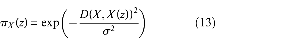
To address this issue, local interpretable model-agnostic explanations (LIME) is applied in this study to explain the basis of deep learning models in detecting fastener failure.⁵⁸ The core concept of LIME is to assess how the performance of the predictive model changes when the data are perturbed. A new dataset is then created by generating perturbed samples and their corresponding predictions. Then, a model is trained on this new dataset, where the instances are weighted based on their proximity to the instance being explained. This approach helps identify which input features the model relies on to make its prediction. This process can be described as follows^59,60:

ξ (x) = \underset{g \in G}{argmin} {L (f, g, w^{x}) + ω (g)}

(9)

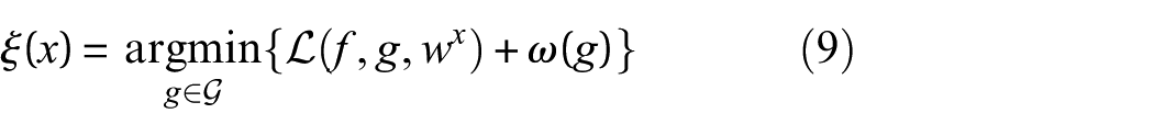
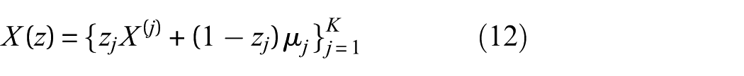
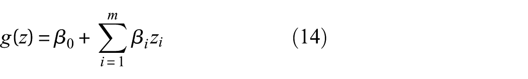
where g denotes the explanation model for the instance x, and $G$ represents the set of possible explanation models. $L$ is the loss function used to evaluate how closely the predictions from the explanation model match those of the original model. $f$ refers to the original model, while $w^{x}$ defines the weight assigned to the sampled data based on its proximity to the original data. The closer the sampled data is to the original, the higher the weight assigned, and vice versa.

In this study, the input to the deep learning model is signals, which are sequences of data that cannot be processed by traditional LIME. Based on traditional algorithms, we propose a signal-specific LIME technique. This technique divides the input signal into segments of equal length, with each segment’s response considered as a feature of the input, thus forming a new dataset. Specifically, let the original time series be

X = {x_{1}, x_{2}, \dots, x_{T}}

(10)

Divide X into K equal segments:

{X^{(1)}, X^{(2)}, \dots, X^{(K)}}

(11)

For each segment $j = 1, 2, \dots, K$ , define a binary indicator $z_{j} \in {0, 1}$ , and $z_{j} = 1$ means the segment is kept unchanged, $z_{j} = 0$ means the segment is replaced by a baseline value.

The perturbed time series corresponding to a binary vector $z = (z_{1}, z_{2}, \dots, z_{K})$ is defined as follows:

X (z) = {z_{j} X^{(j)} + (1 - z_{j}) μ_{j}}_{j = 1}^{K}

(12)

Define the weight for a perturbed sample $X (z)$ as follows:

π_{X} (z) = \exp (- \frac{D {(X, X (z))}^{2}}{σ^{2}})

(13)

where $D (x, z)$ is a distance metric between the original instance x and the perturbed sample z, $σ$ is a scaling parameter controlling the decay of the weight with respect to the distance. The local explanation model in the time series setting is given by

g (z) = β_{0} + \sum_{i = 1}^{m} β_{i} z_{i}

(14)

where $z_{i}$ represents the ith feature of the perturbed sample z, $β_{i}$ indicates the contribution (coefficient) of the ith feature, and $β_{0}$ is the intercept term.

To train the explanation model, the loss function is defined as follows:

L (f, g, π_{X}) = \sum_{z \in Z} w^{x} (z) {[f (X (z)) - g (z)]}^{2}

(15)

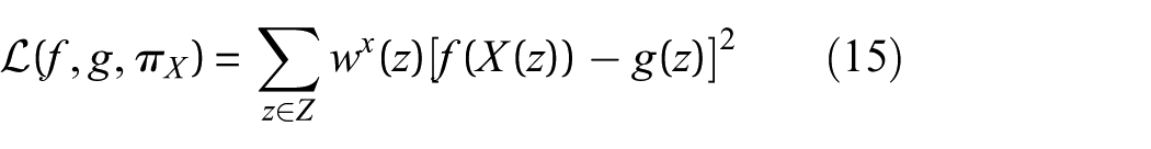
where the summation is over the set of perturbed samples Z. The final optimization problem for the time series explanation is

ξ (X) = \arg min_{g \in G} L (f, g, π_{X}) + Ω (g)

(16)

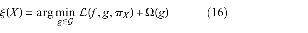
Subsequently, LIME constructs and trains an interpretable model on this dataset, which can be used to assess the contribution of each signal segment to the prediction.

Field experiments and signal analysis

In this section, a field experiment on rail fastening failure was conducted. “Experimental setup” section provides a detailed introduction to the experiment site, equipment, deployment, and conditions. “Experimental results” section presents the response results measured by the accelerometers and the DAS system, along with a detailed comparison and analysis of these results.

Experimental setup

The conditions at the experimental site and the layout of the sensors are shown in Figure 4. Five accelerometers were installed on the rail waist and rail foot, each capable of measuring the acceleration response in three directions, and the DAS optical fiber was deployed on the rail foot, which was fixed by adhesive tapes in order to be tightly attached to the rail foot. The hammer loading position was located between the fastener #a and the fastener #b. The positions of the five accelerometers are shown in Figure 4(a). In the DAS system, the six SPs closest to the hammer impact (labeled SP-A to SP-F) were selected for response analysis in this study. Among them, SP-B to SP-E are explicitly marked in the figure, while SP-A and SP-F are located on either side of the impact point and are the farthest from it. It is important to note that each SP in the DAS system does not correspond to a single physical location. Instead, it represents an aggregated response over a certain segment of the optical fiber, obtained by spatially integrating the signal along that segment. Thus, each SP can be regarded as a virtual sensor covering a specific distance.

Figure 4.

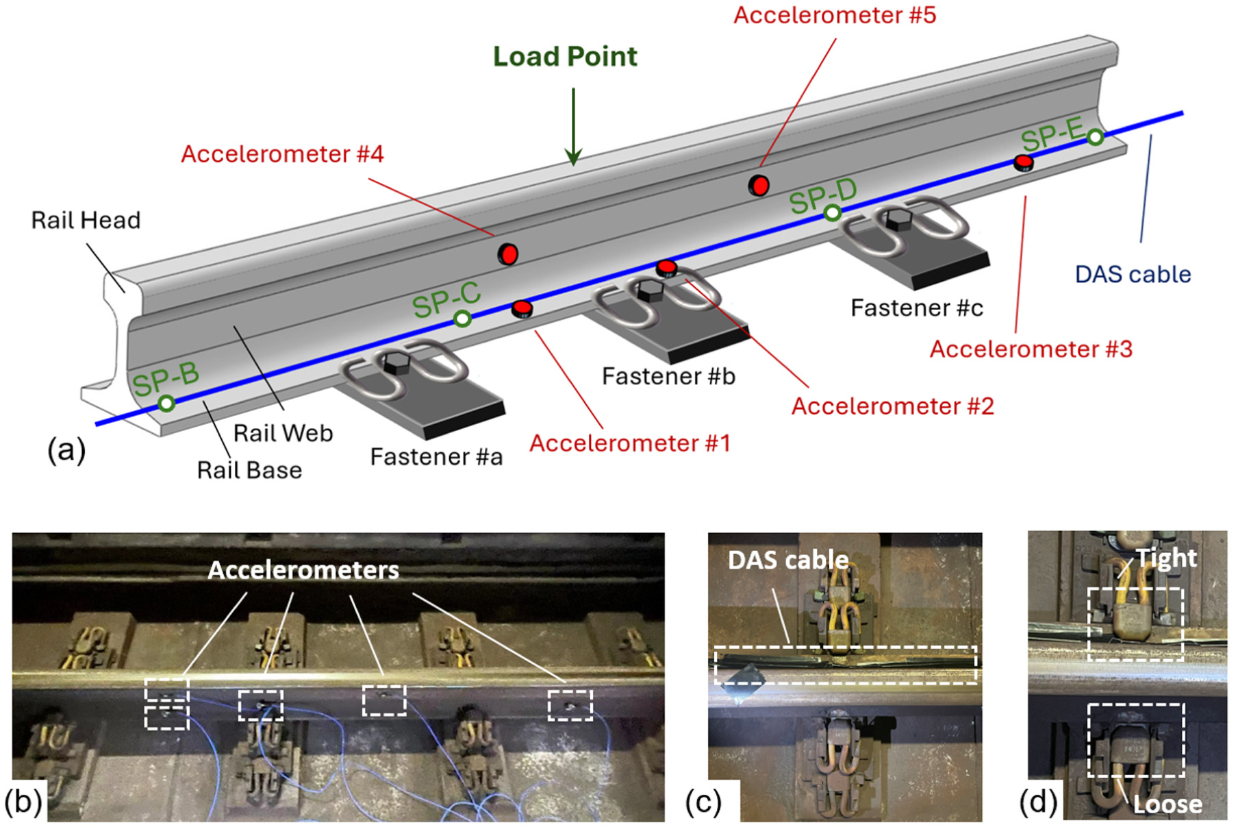
Hammer test setup for the track and sensor layout: (a) schematic diagram of sensor and hammering positions, (b) field view of accelerometers layout, (c) field view of accelerometers layout, and (d) field view of tight and loose fastening conditions.

The equipment involved in this experiment is shown in Figure 5. Specifically, PCB model 086D20 impacts hammer (PCB Piezotronics, Depew, NY, USA) was used to provide the excitation force for the rail, and PCB model 356A25 accelerometer (PCB Piezotronics, Depew, NY, USA) was used for this experiment with a measurement range of 200 g, and the NI-9234 data acquisition module is used to acquire acceleration signals. The AP sensing N52 DAS system (AP Sensing GmbH, Böblingen, Germany), including the interrogator unit and the data processing unit, is used in this experiment to send laser pulses into the fiber-optic cable, as well as to collect and process signal data.

Figure 5.

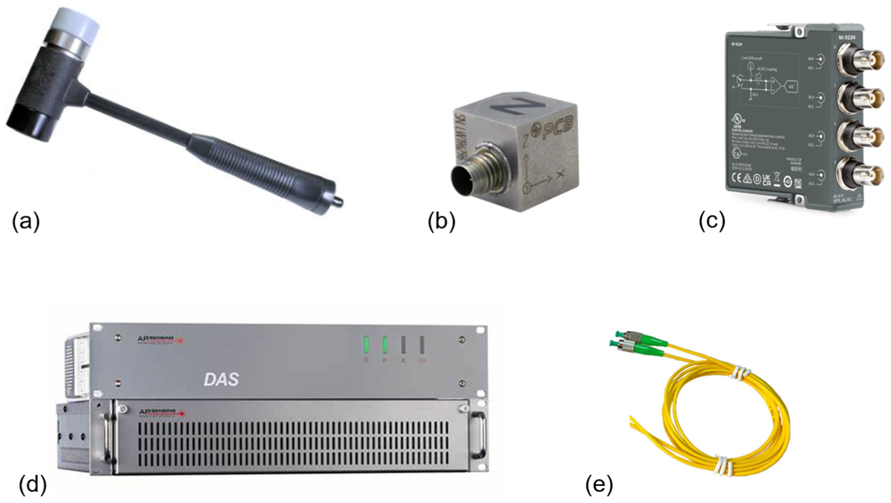
Equipment involved in the field experiment: (a) impact hammer, (b) accelerometer, (c) accelerometer data acquisition module, (d) DAS interrogator unit and processing unit, and (e) fiber-optic cable.

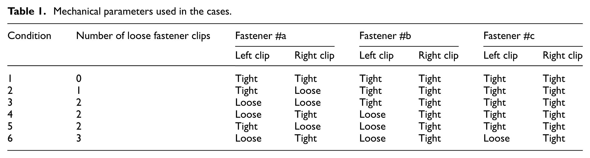
In this experiment, six working conditions were set up to characterize various fastener failure conditions, which are shown in Table 1. Specifically, in condition 1, all the fastener strips were fastened, which represented the normal condition as the control group. The rest of the conditions represent abnormal conditions, that is, some of the fastener strips were loosened. The highest number of loosened fastener strips occurred in condition 6, where three fastener strips were loosened. A field view of the tight and loose fastener strips is shown in Figure 4(d).

Table 1.

Mechanical parameters used in the cases.

Condition	Number of loose fastener clips	Fastener #a		Fastener #b		Fastener #c
Condition	Number of loose fastener clips	Left clip	Right clip	Left clip	Right clip	Left clip	Right clip
1	0	Tight	Tight	Tight	Tight	Tight	Tight
2	1	Tight	Loose	Tight	Tight	Tight	Tight
3	2	Loose	Loose	Tight	Tight	Tight	Tight
4	2	Loose	Tight	Loose	Tight	Tight	Tight
5	2	Tight	Loose	Loose	Tight	Tight	Tight
6	3	Loose	Tight	Loose	Tight	Loose	Tight

Experimental results

Figure 6 shows the hammer impact load acquired in the experiment and the dynamic response measured by the accelerometer and DAS. Specifically, the dynamic response mainly consists of the forced vibration response of the rail under the hammer impact load and the free vibration response of the rail without external load afterward. From Figure 6(a), it can be seen that the load is applied to the structure for about 0.005 s, at which moment the responses measured by both accelerometers and DAS peak, while its dynamic response gradually decays for most of the subsequent time. The RMS values of the accelerometer and DAS measured responses are also shown in Figure 6(b) and (c), respectively. It can be noticed that the dynamic response of both sensors decays rapidly around the first 0.2 s, which is marked as a gray area, and gradually stabilizes thereafter. This stabilized value is considered as the background noise of the test site. It can be seen that the noise in the DAS measurements is significantly larger than that measured by the accelerometer, which may be due to the fact that the DAS is more sensitive to ambient sound, including sounds caused by mechanical equipment and human activities in the test site. Also, since it is a distributed measurement system, the signal from each sampling point is actually a combined reflection of vibration and sound within a certain range near that point, rather than a strictly single-point measurement, and thus may be more widely affected by environmental factors. To reduce the effect of ambient noise on the signal analysis, the time period of rapid decay of the response obtained from both sensors was extracted for subsequent response analysis, that is, the first 0.2 s.

Figure 6.

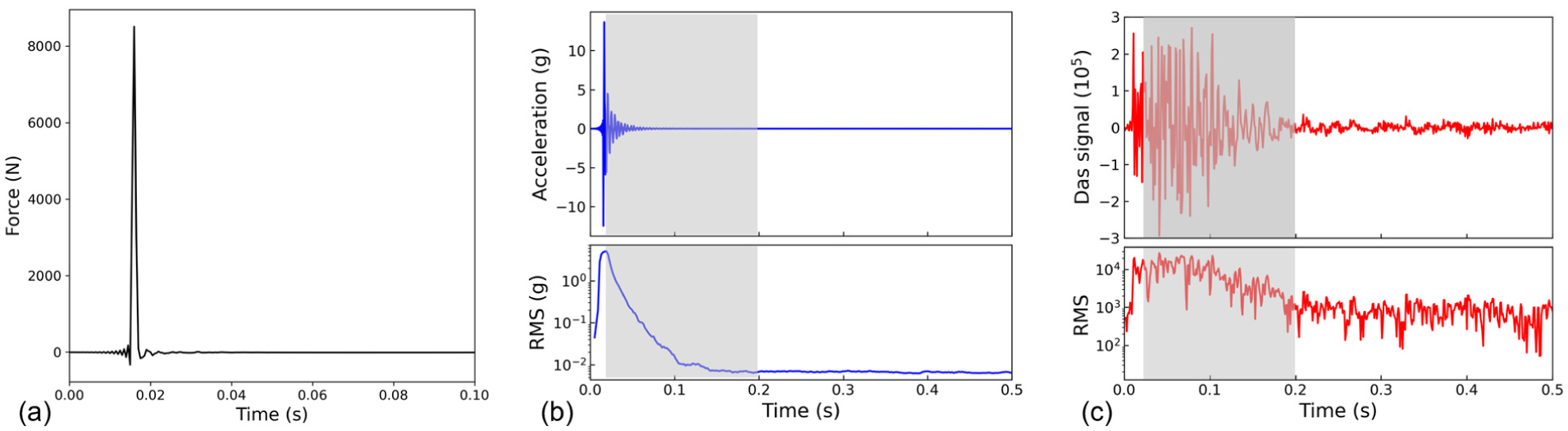
The typical signal obtained from a hammer impact test: (a) hammer impact force signal, (b) acceleration signal, and (c) DAS signal. DAS: distributed acoustic sensing.

The typical spectrum of the free vibration responses of the rail in the vertical, lateral, and longitudinal directions under hammering loads are shown in Figures 7 to 9. It can be found that the trend of the spectra of the responses measured at different locations is relatively consistent, that is, the vertical vibration of the rail reaches a peak near 265 Hz and the lateral vibration reaches a peak near 112 Hz when the clip is tightened. These two frequencies are considered to be the first-order natural frequencies of the rail in different directions, which is consistent with the results in exiting researches.^2–4 At this modal frequency, the rail undergoes in-phase motion across all positions, which can be mechanically modeled as a simplified mass-spring system. In other conditions, the fastener clips of the rails are loosened and the natural frequency of the rails is reduced in both directions. Specifically, in condition 6, when the three fastener clips are loosened, the vertical natural frequency of the rail is reduced to approximately 230 Hz and the lateral natural frequency is reduced to approximately 102 Hz. This is because, in the mechanical system of the rail, the rubber fastener pads provide elastic support for the rail. The main function of the fastener clip in the system is to provide sufficient downforce for the rail, thus ensuring close contact between the rail and the fastener pad. Therefore, when the clip is loosened, the support effect of the fastener plate on the rail is weakened, which can be regarded as a reduction in the elastic modulus of the elastic support in the mechanical system, resulting in a reduction in the natural frequency of the system.

Figure 7.

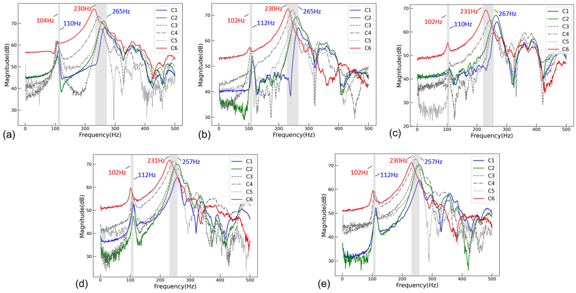
The frequency spectrum of the vertical dynamic response of each accelerometer under different conditions (the condition is labeled as C in the legend): (a) accelerometer #1, (b) accelerometer #2, (c) accelerometer #3, (d) accelerometer #4, and (e) accelerometer #5.

Figure 8.

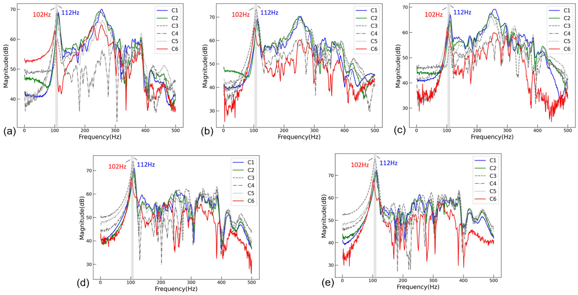
The frequency spectrum of the lateral dynamic response of each accelerometer under different conditions (the condition is labeled as C in the legend): (a) accelerometer #1, (b) accelerometer #2, (c) accelerometer #3, (d) accelerometer #4, and (e) accelerometer #5.

Figure 9.

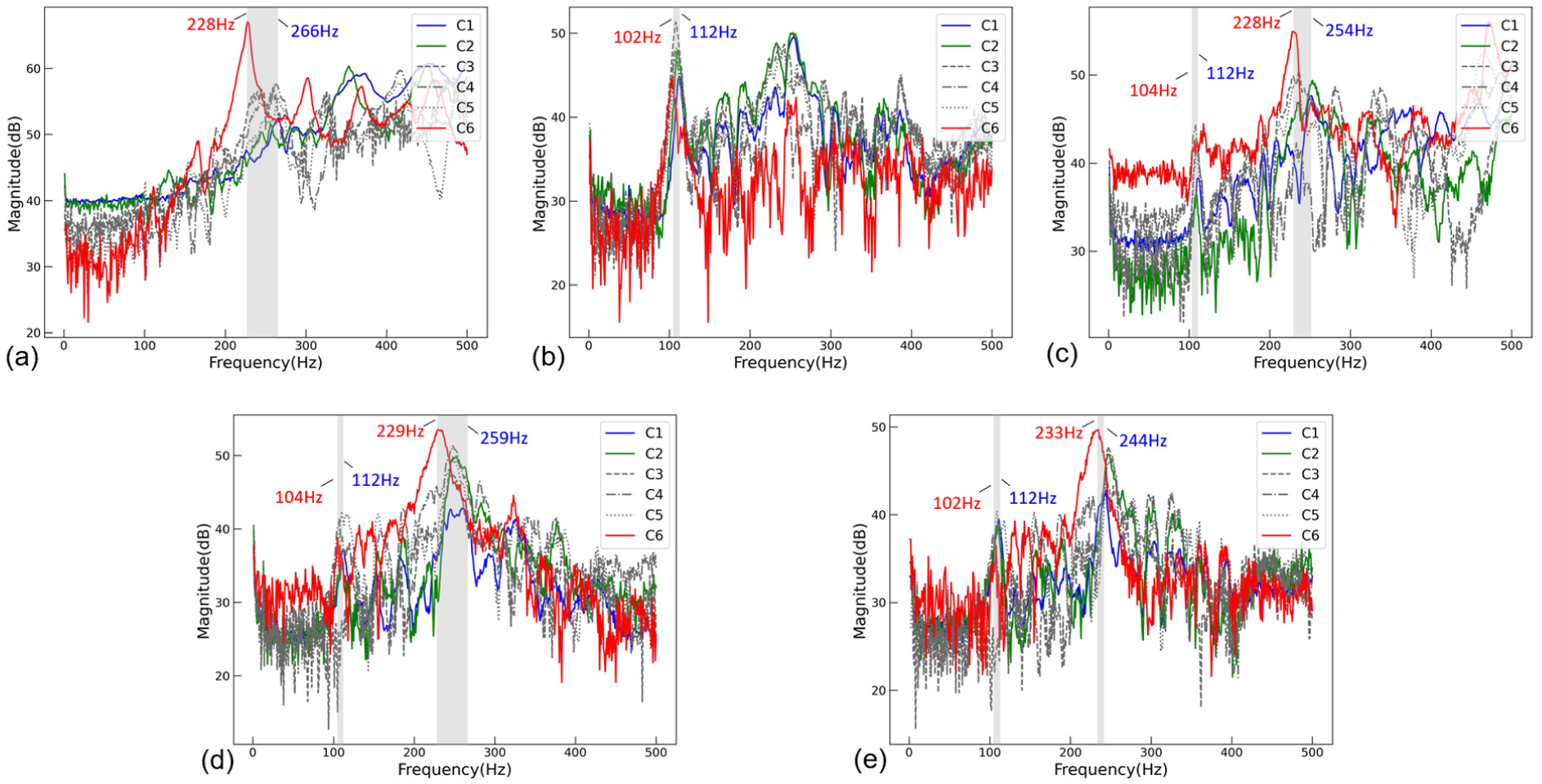
The frequency spectrum of the longitudinal dynamic response of each accelerometer under different conditions (the condition is labeled as C in the legend): (a) accelerometer #1, (b) accelerometer #2, (c) accelerometer #3, (d) accelerometer #4, and (e) accelerometer #5.

In this experiment, the responses measured at the six SPs of the DAS close to the hammering point were used for the analysis, and the spectrum of the responses measured by the DAS at different conditions is illustrated in Figure 10. It can be seen that the DAS response for all conditions shows a significant peak near 50 Hz, where no significant response is observed for the acceleration signal. The phenomenon is considered to be related to the installation method of the fiber-optic cable, as the fiber optic is glued on the surface of the rail, which leads to insufficient transmission of the vibration response from the rail to the fiber optic, which may result in a significant response of 50 Hz that is not measured by the rail accelerometers.

Figure 10.

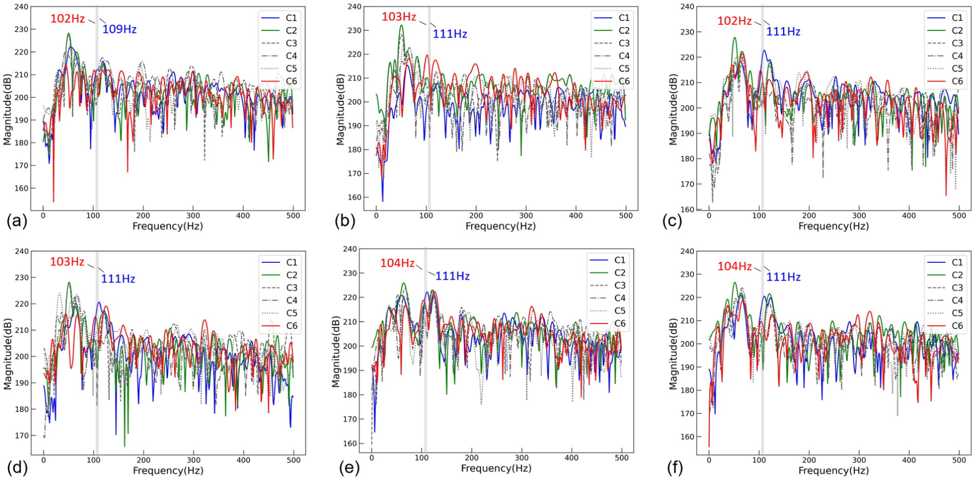
The frequency spectrum of the responses measured at each SP of the DAS system under various operating conditions (the condition is labeled as C in the legend): (a) SP-A, (b) SP-B, (c) SP-C, (d) SP-D, (e) SP-E, and (f) SP-F. SP: sensing point; DAS: distributed acoustic sensing.

In addition, compared to the acceleration response, the noise of the response measured by DAS is more significant, especially in the high-frequency band, and its response peaks in many frequency bands without showing significant characteristic trend, and it is difficult to be reasonably interpreted by the mechanical knowledge. This is because DAS measurements are based on fiber-optic interferometry, which senses the environmental vibration and sound through phase changes in fiber-optic transmission. Also, the signal at each DAS SP is not independent, but is a composite reflection of vibrations and sounds in the area adjacent to a section of fiber, which makes it more susceptible to ambient noise. In addition, the signal at each SP is usually spatially smoothed by interpolation or filtering processing, which also results in the high-frequency signal being attenuated while the low-frequency noise component is amplified.

However, it can be noticed that although not particularly significant, the peak of the DAS signal near 100–110 Hz also varies with the conditions, showing a similar trend to the lateral acceleration response of the rails. Whereas, at the vertical natural frequency of the rail, that is, around 250 Hz, the DAS signal is much noisier and therefore does not show a significant pattern. The above phenomenon shows that DAS signals are not as easy to interpret as acceleration signals due to different acquisition principles, but its response also contains some responses related to structural dynamic characteristics, which can also be measured by accelerometers. This implies that more complex methods, such as machine learning methods, need to be carried out in the research of DAS-based structural anomaly diagnosis and detection in order to fully exploit the physical information embedded in the signals.

Model performance and analysis

In this section, the performance of the deep learning model on data obtained from field experiments is conducted and discussed. Specifically, “Model implementation” section provides a comprehensive description of the model implementation, including dataset preprocessing, the configuration of deep learning model parameters, and performance evaluation metrics. “Performance based on individual data source” section presents the performance of models trained using acceleration signals and DAS signals independently, along with an evaluation of these results using interpretability techniques. “Performance based on cross-modal transfer learning” section discusses the performance of the deep learning model trained with the proposed cross-modal transfer learning method, accompanied by an in-depth analysis and discussion of the findings.

Model implementation

Based on the method proposed in the second section, deep learning models were developed using only DAS signals, only acceleration signals, as well as the proposed cross-modal transfer learning framework. The field experimental data obtained in the third section were randomly divided into training, validation, and test datasets in a ratio of 7:1:2. These datasets were used to train and evaluate the developed deep learning models. Specifically, the training set was used to fit the model, the validation set was used to monitor overfitting and determine the optimal model checkpoint during training, and the test set was used to evaluate the final performance of the trained models. To reduce the randomness introduced by a single data split and enhance the robustness of the evaluation results, the dataset was randomly partitioned five times, and model training and testing were conducted independently on each split. Specifically, for the acceleration signals, the input to the model consisted of the spectral data of the acceleration responses in three directions measured by one accelerometer. For the DAS signals, the data from the six SPs closest to the impact zone were used as the input to the deep learning model.

The encoders for both acceleration and DAS signals are CNN and Transformer modules. Specifically, the CNN consists of three one-dimensional convolutional layers with kernel size 3 and filter sizes of 256, 128, and 64, respectively, enabling effective feature extraction and compression from the raw input. Each layer uses LeakyReLU activation followed by batch normalization to improve training stability. A max pooling layer is applied after the CNN to further reduce the temporal dimension. The transformer component comprises three stacked blocks, each containing a four-head multihead self-attention mechanism with a model dimension of 64, along with a feedforward neural network, residual connections, and layer normalization to enhance temporal modeling capability and stability. Dropout layers are incorporated in all transformer blocks to mitigate overfitting. After temporal features are extracted by the encoder, a fully connected regression module is applied. This module begins with a flattening layer, followed by two dense layers with 128 and 32 units, respectively, using LeakyReLU activation and dropout for regularization. Finally, a sigmoid-activated output layer predicts the FFI value.

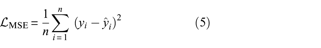
In the model training, the Adam optimizer⁶¹ was employed in conjunction with a dynamic learning rate strategy, where the learning rate gradually decreased from 1e-3 to 1e-4 to enhance the convergence efficiency and stability of the model. The initial number of training iterations for each model was set to 2000, and the iteration count was further increased if the training loss had not stabilized. A batch size of 20 was used during training. Additionally to mitigate overfitting to the training data, the model checkpoint with the lowest validation loss observed during training was selected as the final model.⁶² To comprehensively evaluate the model performance, MSE was used as the evaluation metric, quantifying the model’s prediction accuracy on the test set, which is defined as follows:

MSE = \frac{1}{N} \sum_{i = 1}^{N} {(y_{i} - {\hat{y}}_{i})}^{2}

(17)

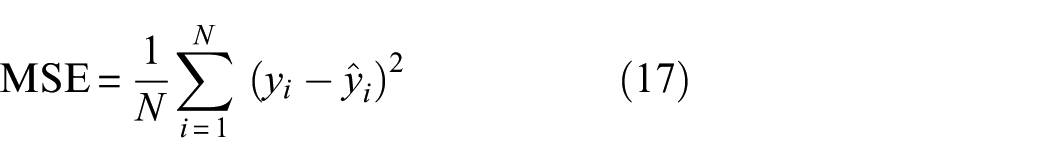
where N represents the number of samples, ${\hat{y}}_{i}$ represents the model’s predicted values, and $y_{i}$ represents the true values.

In addition to MSE, several classification metrics were adopted, including classification accuracy, macro-averaged precision, recall, and F1 score. Since the ground truth values are discrete while the predicted values are continuous, each predicted value was first mapped to the nearest discrete class label. Accuracy was then calculated as the ratio of the number of correct predictions to the total number of samples:

Accuracy = \frac{N_{correct}}{N}

(18)

To better capture performance across all classes, especially in the case of class imbalance, macro-averaged precision, recall, and F1 score were also calculated. These metrics are defined as follows:

{Precision}_{macro} = \frac{1}{C} \sum_{i = 1}^{C} \frac{{TP}_{i}}{{TP}_{i} + {FP}_{i}}

(19)

{Recall}_{macro} = \frac{1}{C} \sum_{i = 1}^{C} \frac{{TP}_{i}}{{TP}_{i} + {FN}_{i}}

(20)

F 1_{macro} = \frac{1}{C} \sum_{i = 1}^{C} \frac{2 \cdot {Precision}_{i} \cdot {Recall}_{i}}{{Precision}_{i} + {Recall}_{i}}

(21)

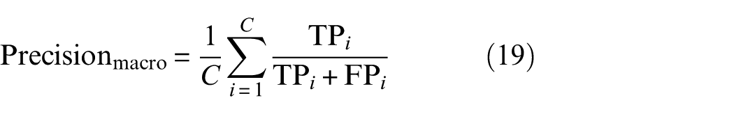
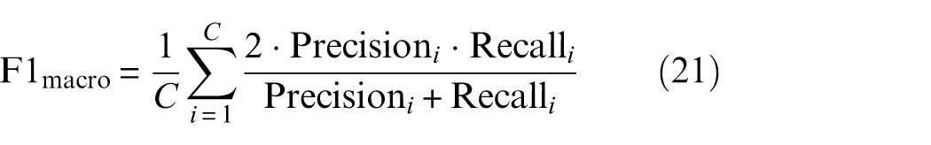
where C is the total number of classes, and TP _i , FP _i , and FN _i denote the numbers of true positives, false positives, and false negatives for class i, respectively. Macro-averaging ensures that each class contributes equally to the overall score, regardless of its frequency in the dataset.

Moreover, the coefficient of the ED loss term $λ$ was set as the reciprocal of its initial value, ensuring that it remains numerically comparable to the main loss component at the start of training. In the development of the interpretable deep learning model, the raw signals were segmented into intervals of 5 Hz, meaning that, in the subsequent calculation of the contribution of each frequency band to the prediction, each 5 Hz interval was treated as an individual feature. In addition, the number of samples used to generate the local surrogate model is set to 5000. This means that, during each explanation process, LIME perturbs the original input data to generate 5000 distinct samples, which are then used to train a local surrogate model. This approach helps capture the predictive patterns and decision boundaries of the original model.

Performance based on individual data source

Figure 11 illustrates the loss curves of the accelerometer-based and DAS-based models during a representative training process. Both models show convergence in training and validation losses within 2000 epochs, indicating the adequacy of the selected training duration. Overall, the DAS-based model exhibits more pronounced overfitting, while its training loss continues to decrease, the validation loss initially declines but later fluctuates significantly with an upward trend. In contrast, the validation loss of the accelerometer-based model also fluctuates but generally shows a downward and convergent trend. This is likely due to higher noise levels in the DAS signals, which make the model more prone to fitting noise patterns in the training data, thereby reducing generalization ability and leading to overfitting. To mitigate this issue, the model checkpoints corresponding to the lowest validation loss were selected for subsequent evaluation, which occurred at epoch 1772 for the accelerometer-based model and epoch 1262 for the DAS-based model.

Figure 11.

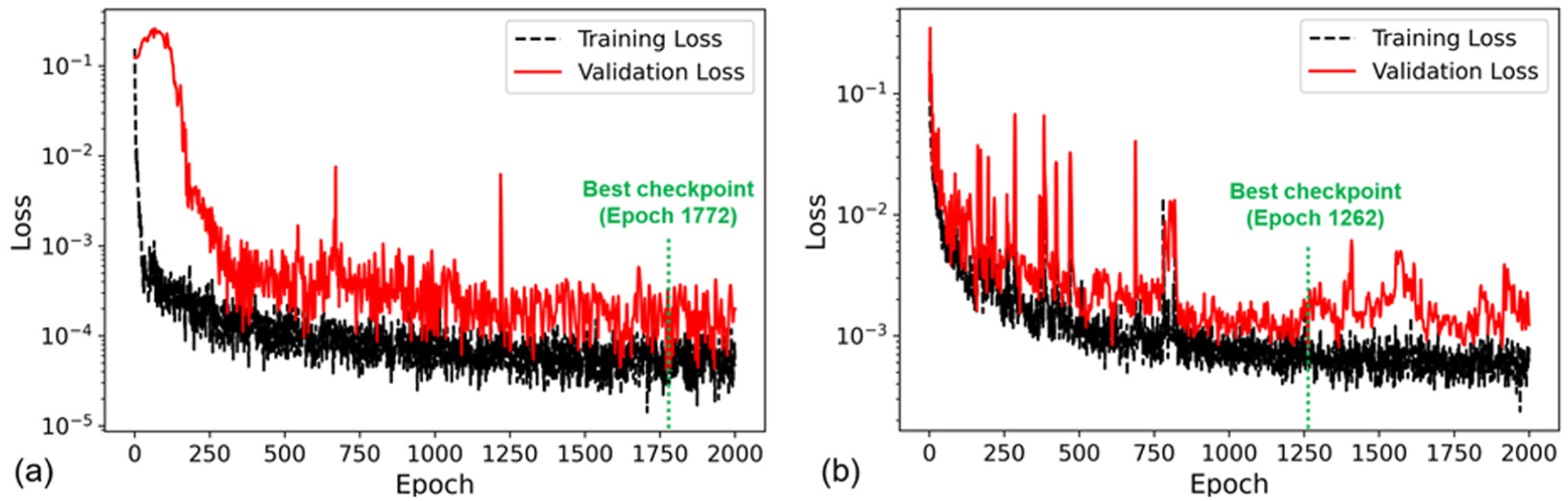
Training and validation loss curves: (a) accelerometer-based model and (b) DAS-based model. DAS: distributed acoustic sensing.

Table 2 presents a performance comparison between the DAS-based and accelerometer-based models on the test set. In terms of MSE, the accelerometer-based model significantly outperforms the DAS-based model, with an average MSE of 3.86 × 10⁻⁵ compared to 4.52 × 10⁻³. Similarly, the classification accuracy of the accelerometer-based model is higher, achieving an average of 99.50%, while the DAS-based model reaches an average of 94.00%. These results indicate that the accelerometer-based model can accurately predict the FFI using rail response signals. Although the DAS-based model also achieves reasonable accuracy, its overall performance is lower. This is likely due to the higher signal-to-noise ratio and stability of accelerometer signals, which facilitate the extraction of informative features. In contrast, DAS signals are more susceptible to coupling quality and environmental noise, which may lead to overfitting during training and reduce the model’s generalization ability on unseen data.

Table 2.

Performance comparison between DAS-based and accelerometer-based models on the test set.

Performance metric	DAS only	Accelerometer only
MSE: average (Std)	4.52E-03 (2.44E-03)	3.86E-05 (2.44E-05)
Accuracy: average (Std)	94.00% (1.37E-02)	99.50% (1.12E-02)
Precision (macro): average (Std)	92.27% (2.18E-02)	98.75% (2.80E-02)
Recall (macro): average (Std)	91.11% (2.83E-02)	99.64% (7.99E-03)
F1 score (macro): average (Std)	91.58% (2.50E-02)	99.10% (2.01E-02)
Key frequency for prediction	52 Hz, 67 Hz	112 Hz, 247 Hz

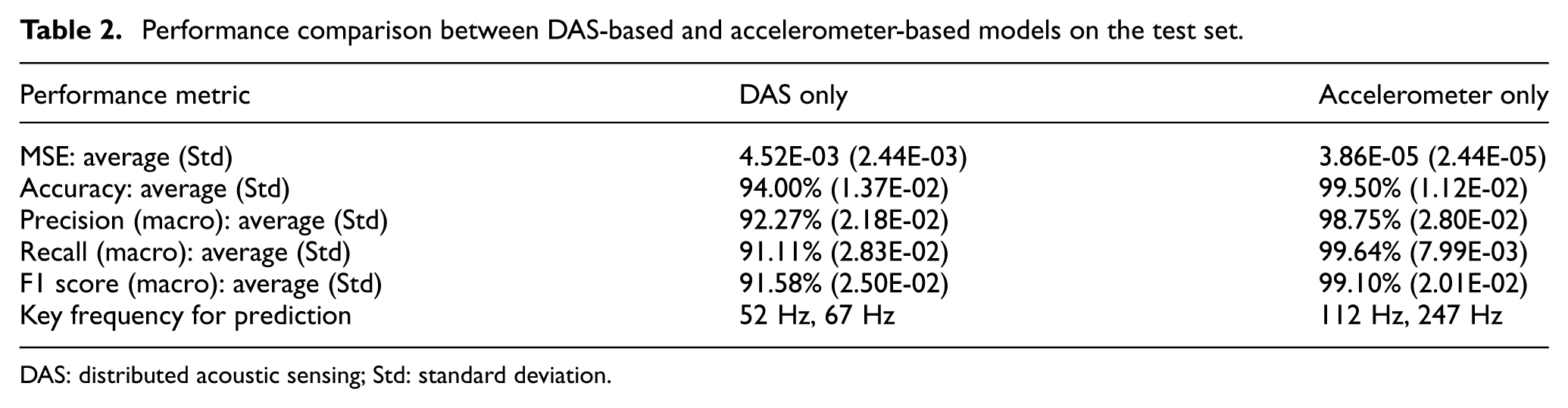
DAS: distributed acoustic sensing; Std: standard deviation.

Figures 12 and 13 show the contributions of different frequency bands in the acceleration signals to the model predictions, obtained using interpretability techniques. Positive contributions are represented by red bars, indicating that the feature increases the predicted FFI value, while negative contributions are represented by green bars, indicating that the feature decreases the predicted FFI value.

Figure 12.

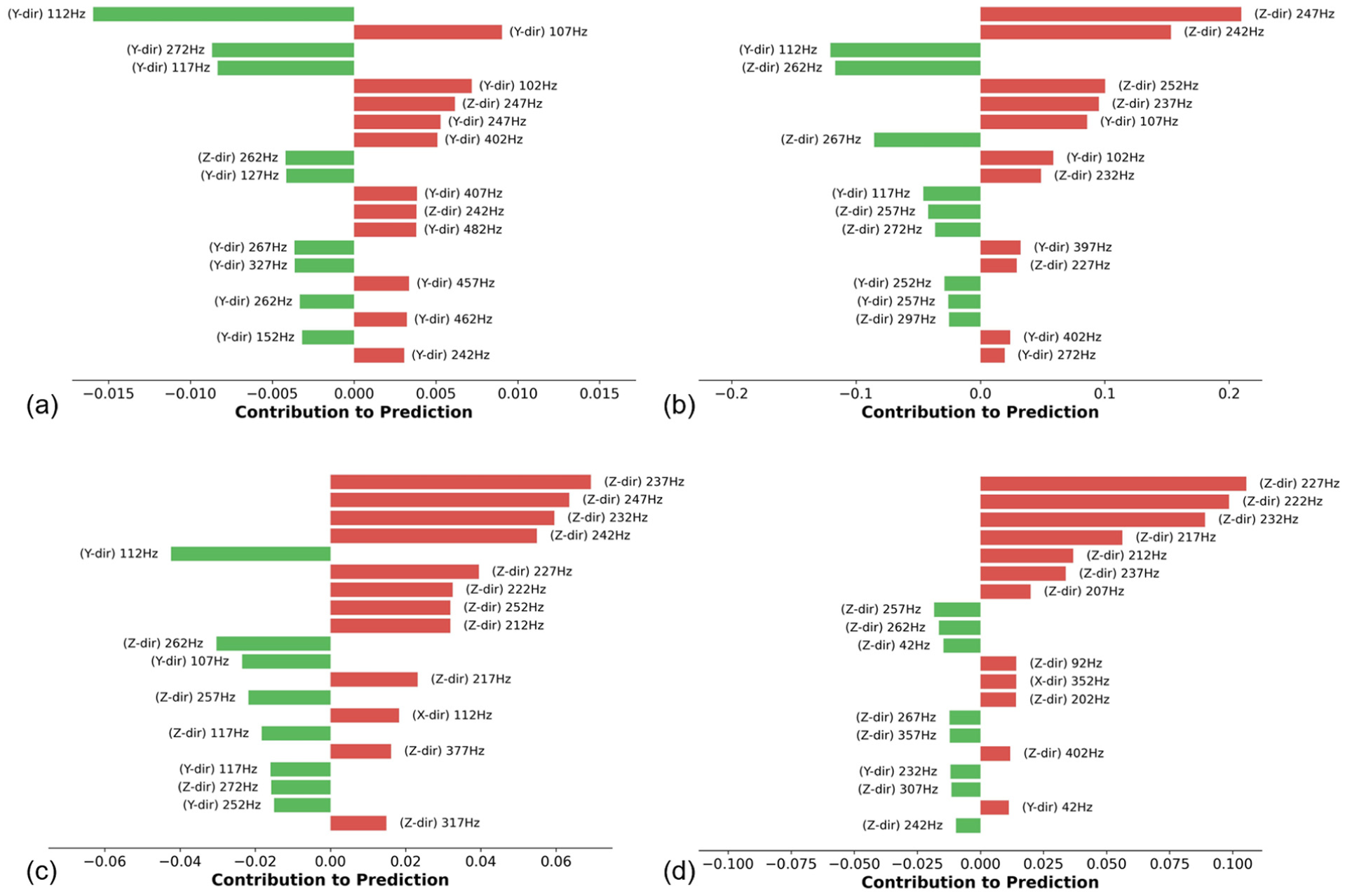
The contribution of various frequency features of the acceleration signal to the results of the model predictions, which were derived using the LIME technique. These features are represented by frequencies in the X, Y, and Z directions, ordered by their contribution to the predictions. The different panels represent samples from different conditions: (a) FFI = 0, (b) FFI = 1, (c) FFI = 2 and (d) FFI = 3. LIME: local interpretable model-agnostic explanations; FFI: fastener failure index.

Figure 13.

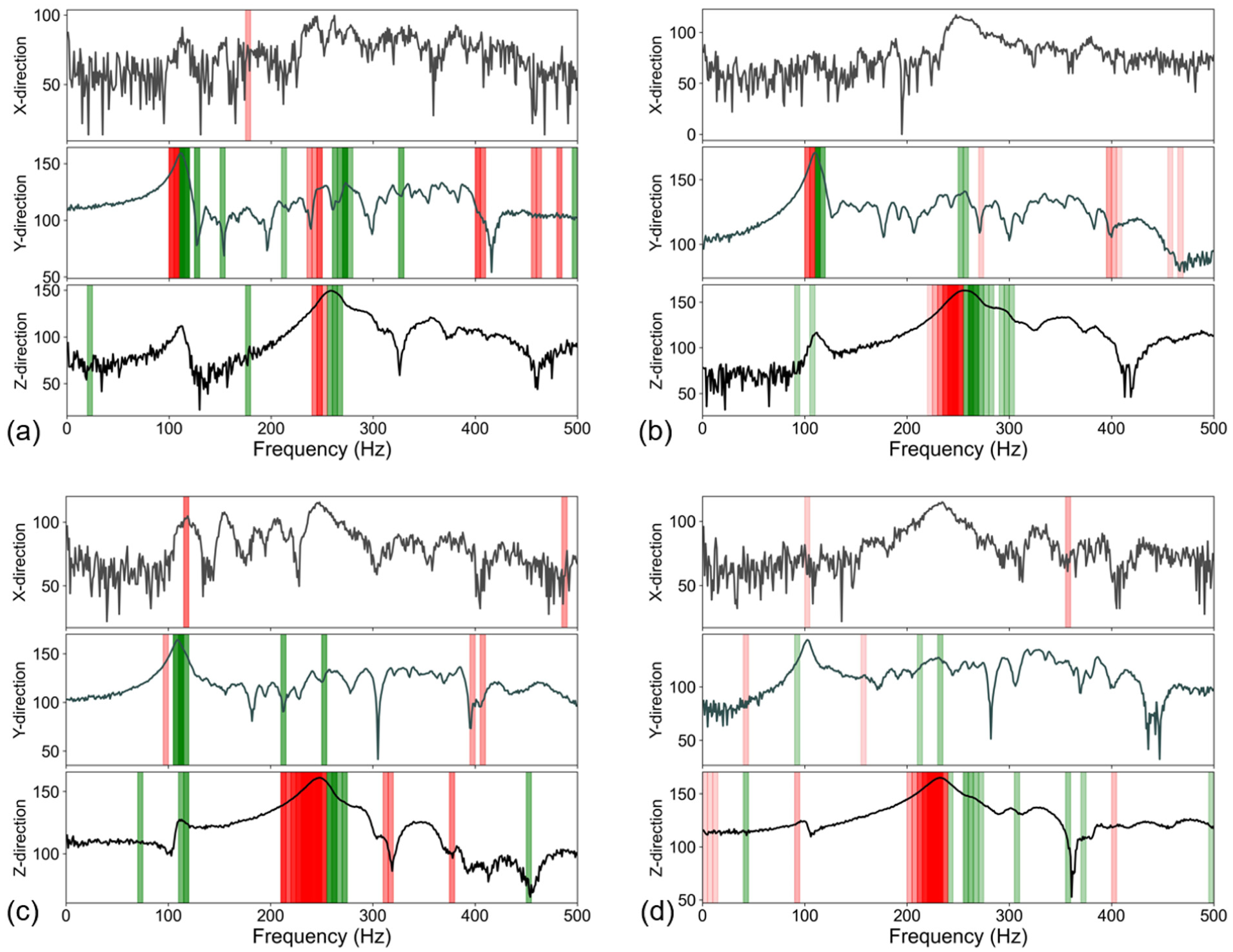
The spectra of acceleration signals in the X, Y, and Z directions for each conditions, with colored vertical bars overlaid on the spectra indicating the contribution of specific frequency bands identified by LIME: (a) FFI = 0, (b) FFI = 1, (c) FFI = 2 and (d) FFI = 3. LIME: local interpretable model-agnostic explanations; FFI: fastener failure index.

It can be observed from the figures that the response frequency bands contributing the most to the model predictions are primarily concentrated in the 220–270 Hz vertical response band and the 100–115 Hz lateral response band, which are consistent with the natural frequencies of the rail in both directions as analyzed in the third section. Specifically, as shown in Figure 13, the vertical response in the 220–250 Hz frequency band generally has a positive contribution to the FFI prediction, while in the 250–270 Hz frequency band, it has a negative contribution. This indicates that the greater the response in the 220–250 Hz band, the higher the predicted FFI, meaning a greater number of rail fastener failures. Conversely, the greater the response in the 250–270 Hz band, the lower the predicted FFI, meaning fewer rail fastener failures. This aligns perfectly with the analysis based on physical knowledge in the third section. The same phenomenon is also observed in the contributions of different frequency bands of the lateral acceleration response. From these results, it can be seen that the deep learning model trained with acceleration data utilizes certain features for detecting the rail FFI that are consistent with the underlying physical knowledge. This performance is considered to exhibit high robustness and generalization, indicating that the trained model can be fully applied to rail fastener failure detection in other datasets under similar conditions.

Figures 14 and 15 illustrate the contributions of different frequency bands in the DAS signals to the model predictions, obtained using interpretability techniques. From the figures, it can be found that the frequency bands contributing most to the model predictions in the DAS signals are primarily concentrated in the 40–70 Hz range for each node, which corresponds to the main peaks in the DAS signal spectrum. However, responses in frequency bands related to the natural frequencies of the rail were almost not utilized by the deep learning model in the prediction. This indicates that although the model achieved high prediction accuracy on the test dataset, the basis for its predictions does not align with the physical principles underlying rail fastener failure. This could be because the DAS system captured other information near 50 Hz that is indirectly related to rail fastener failure. Additionally, this might suggest the presence of overfitting during model training. In cases of small sample sizes, the model may exhibit an excessive reliance on specific frequency features, which could be incidental noise or unique patterns in the data rather than truly critical features. Such overfitting may result in performance degradation when the model encounters other unseen data, limiting its generalizability. Therefore, it is necessary to implement measures to mitigate overfitting in the deep learning model based on DAS signals, guiding the model to focus more on responses in frequency bands associated with the natural frequencies of the rail.

Figure 14.

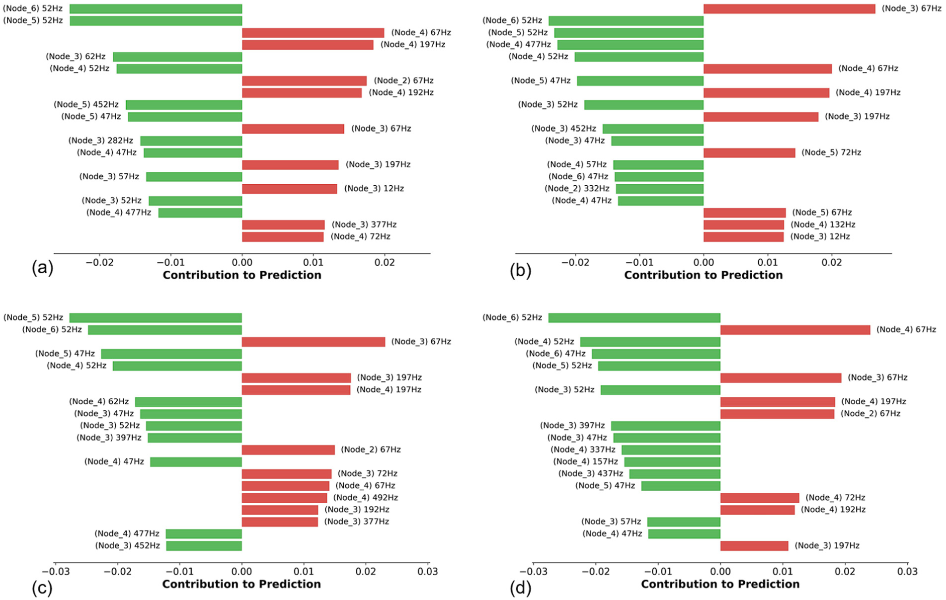
The contribution of various frequency features of the DAS signal to the results of the model predictions, which were derived using the LIME technique. These features are represented by the frequencies of the responses of the six nodes, ordered by their contribution to the predictions. The different panels represent samples from different conditions: (a) FFI = 0, (b) FFI = 1, (c) FFI = 2 and (d) FFI = 3. DAS: distributed acoustic sensing; LIME: local interpretable model-agnostic explanations; FFI: fastener failure index.

Figure 15.

The spectra of DAS signals in six nodes for each condition, with colored vertical bars overlaid on the spectra indicating the contribution of specific frequency bands identified by LIME: (a) FFI = 0, (b) FFI = 1, (c) FFI = 2, (d) FFI = 3. DAS: distributed acoustic sensing; LIME: local interpretable model-agnostic explanations; FFI: fastener failure index.

Performance based on cross-modal transfer learning

Using the proposed cross-modal transfer learning method mentioned in the second section, models were separately established, pretrained, and retrained. Figure 6 illustrates the loss evolution of the proposed cross-modal transfer learning model during a representative training process, including both the pretraining and re-training phases. In Figure 16(a), the model is pretrained using both accelerometer and DAS data by jointly optimizing the MSE and ED losses. To ensure that all loss components sufficiently converge, the total number of training epochs was set to 6000. The results show that the MSE loss converges around epoch 2000, while the ED loss requires a longer period and stabilizes only after approximately 5000 epochs. The best model was obtained at epoch 5872, highlighting the importance of a longer training schedule. Figure 16(b) presents the re-training phase on DAS data. The model, benefiting from pretraining, starts with low training and validation losses, indicating a strong initial capacity to handle DAS signals. The loss continues to decrease slightly in the early phase and then stabilizes. The final model used for evaluation corresponds to the checkpoint with the lowest validation loss at epoch 1848.

Figure 16.

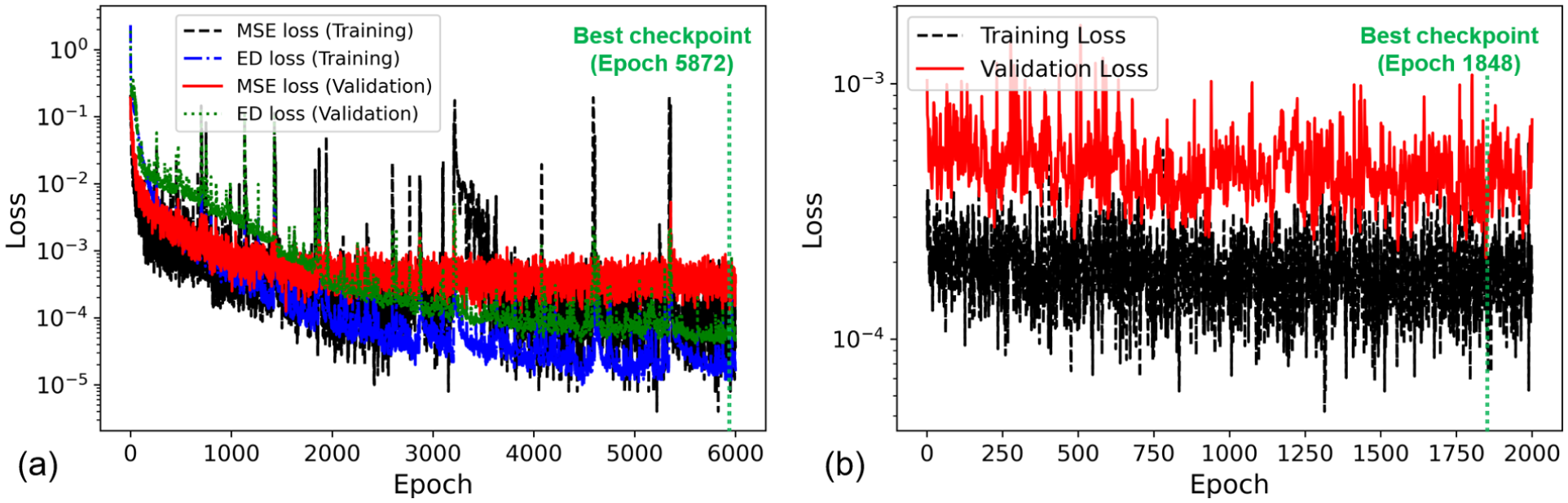
Training and validation loss curves of the proposed cross-modal transfer learning model: (a) loss evolution during the pretraining phase and (b) loss evolution during the re-training phase.

Table 3 compares the performance of the baseline model trained solely on DAS data with the proposed cross-modal transfer learning model on the test set. The results show that the proposed method outperforms the baseline in both MSE and accuracy. Specifically, the proposed model achieves an average MSE of 8.60 × 10⁻⁴ and an average accuracy of 97.50% across multiple evaluations. These results demonstrate that the proposed method, by introducing a constraint mechanism, enables the encoder trained on accelerometer signals to effectively guide feature extraction from DAS signals. This facilitates knowledge transfer and adaptation between different signal modalities, thereby improving prediction performance and enhancing the model’s ability to detect rail fastener failures.

Table 3.

Performance comparison between the DAS-only model and the proposed cross-modal transfer learning model on the test set.

Performance metric	DAS only	Proposed method
MSE: average (Std)	4.52E-03 (2.44E-03)	8.60E-04 (2.29E-04)
Accuracy: average (Std)	94.00% (1.37E-02)	97.50% (1.77E-02)
Precision (macro): average (Std)	92.27% (2.18E-02)	96.21% (2.95E-02)
Recall (macro): average (Std)	91.11% (2.83E-02)	97.24% (2.52E-02)
F1 score (macro): average (Std)	91.58% (2.50E-02)	96.53% (2.33E-02)
Key frequency for prediction	52 Hz, 67 Hz	112 Hz, 247 Hz

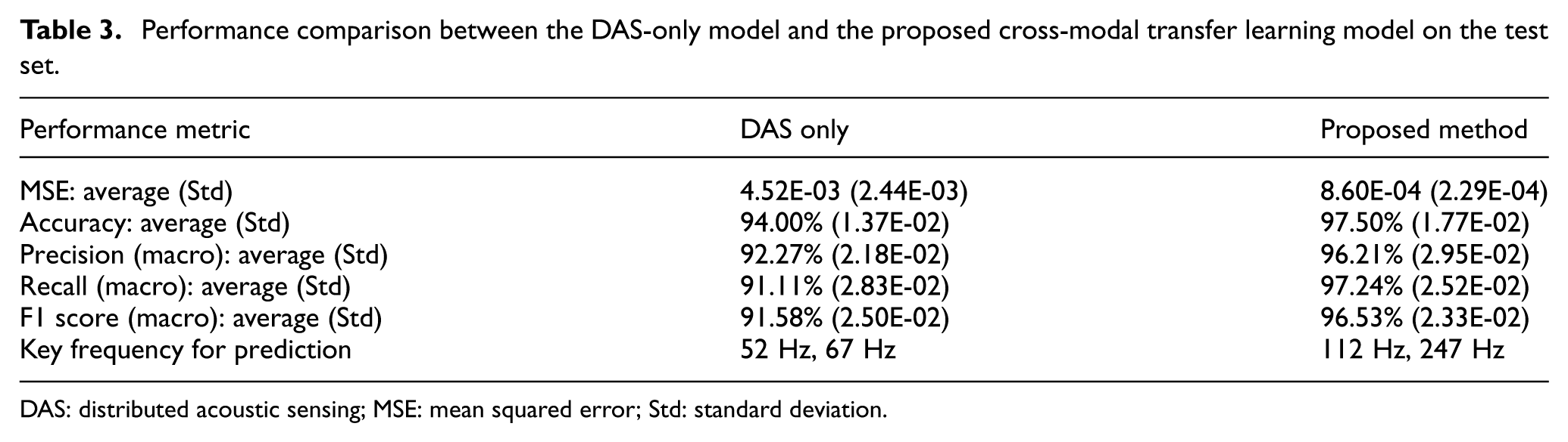
DAS: distributed acoustic sensing; MSE: mean squared error; Std: standard deviation.

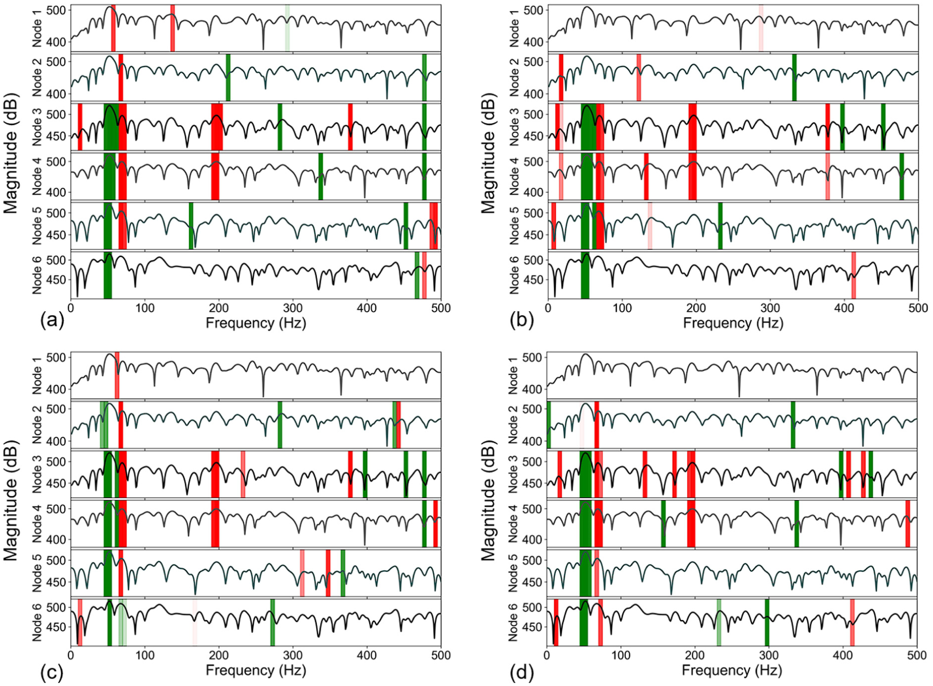
To further investigate the underlying mechanisms behind the improved performance of the proposed cross-modal transfer learning model, we employed the LIME technique to analyze the factors contributing to its predictions. Figures 17 and 18 show the important parts of the DAS signal that contribute to the prediction results after applying the proposed cross-modal transfer learning. As compared to the method shown in Figure 15, which only uses DAS data for training, the model trained with the proposed cross-modal transfer learning method not only relies on the response at 40–60 Hz frequency band but also extracts features from a wider range of frequency bands. Specifically, in the 100–120 Hz frequency band, which corresponds to the lateral natural frequency of the rail, the model trained with proposed method is able to capture the information contained in the acceleration response of rails. This allows the model to account for changes in the mechanical characteristics of the rail under different conditions, which contribute to the robustness of the model, thus significantly improving its robustness.

Figure 17.

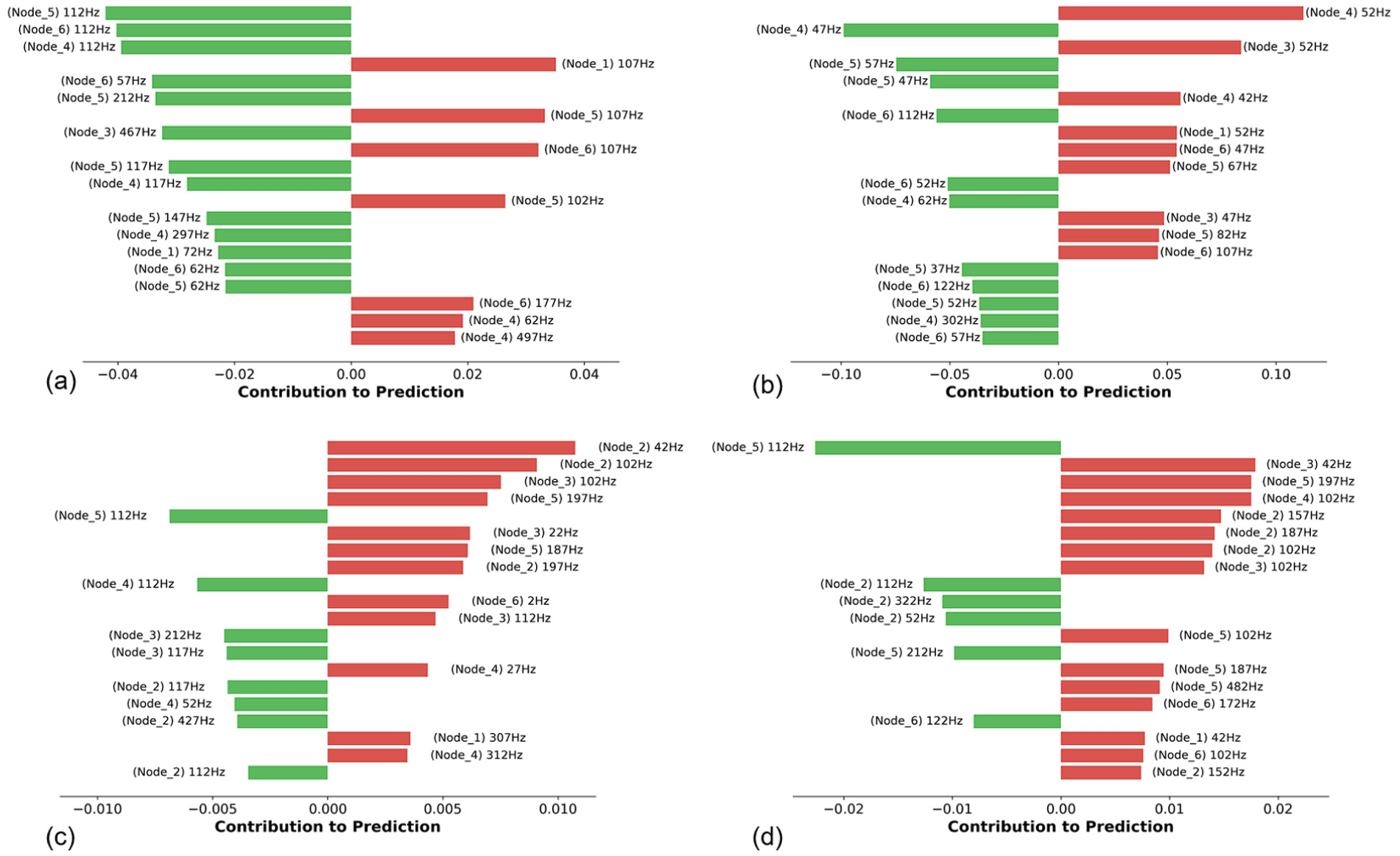
The contribution of various frequency features of the DAS signal to the results of the model predictions using proposed cross-domain adaption method, which was derived using the LIME technique. These features are represented by the frequencies of the responses of the six nodes, ordered by their contribution to the predictions. The different panels represent samples from different conditions: (a) FFI = 0, (b) FFI = 1, (c) FFI = 2 and (d) FFI = 3. DAS: distributed acoustic sensing; LIME: local interpretable model-agnostic explanations; FFI: fastener failure index.

Figure 18.

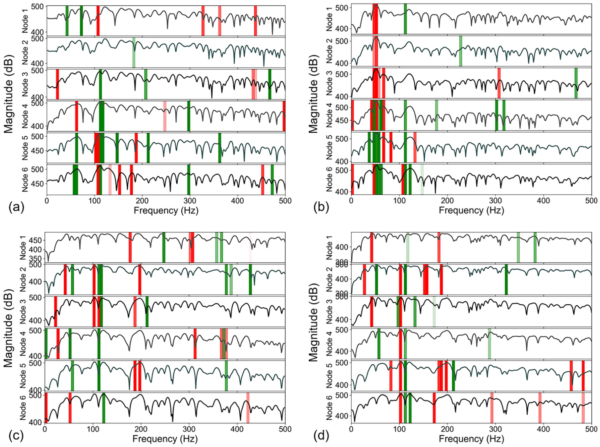
The spectra of DAS signals in six nodes for each condition, with colored vertical bars overlaid on the spectra indicating the contribution of specific frequency bands to the model prediction using proposed cross-domain adaption method: (a) FFI = 0, (b) FFI = 1, (c) FFI = 2 and (d) FFI = 3. DAS: distributed acoustic sensing; FFI: fastener failure index.

Discussion

As indicated by the above analysis, although acceptable accuracy can be achieved using DAS signals alone with deep learning for rail fastener failure detection, the extracted features often lack a strong connection to mechanical principles. Consequently, the generalization capability of such models may be limited—for example, a model trained on one section of the track may not perform well in other locations with different structural or environmental characteristics.

To address this limitation, we propose a cross-modal transfer learning framework that uses physically meaningful features extracted from high-precision, spatially limited point sensors (e.g., accelerometers) to guide feature learning in the DAS-based model. This strategy encourages the model to focus on generalizable characteristics, such as structural natural frequencies, rather than site-specific or noise-sensitive patterns, thereby improving both robustness and interpretability.

At the core of this approach is a physics-guided feature transfer mechanism that enhances the value of distributed sensing. By leveraging high-fidelity local measurements to inform the interpretation of lower-resolution, wide-coverage DAS data, the method is particularly effective in scenarios where dense deployment of high-quality sensors is impractical. This enables more reliable assessment of structural health over large-scale infrastructure systems. Given these advantages, the proposed framework shows strong potential for extension beyond railway applications. Other civil structures, such as bridges, tunnels, and underground facilities, often involve a similar combination of localized high-quality sensors and the need for large-scale distributed monitoring. The proposed method can be readily adapted to such contexts to enable efficient and generalizable anomaly detection.

For practical deployment, we suggest that, alongside the installation of the distributed sensing system, a small number of high-precision sensors be deployed at selected key sections. These point sensors can be used to extract physically relevant features that guide DAS-based analysis through transfer learning, thereby enhancing the model’s adaptability across different track segments and geographic environments.

One limitation of this study is that the experimental data were obtained under artificial excitation, resulting in low levels of ambient noise. Future work will involve field experiments under actual train operation, where the vibration responses are expected to contain more complex and noisy patterns. Addressing this challenge will be essential for promoting real-world adoption of the proposed method.

Conclusions

In this study, a novel DAS-based rail fastener failure detection method is proposed. Specifically, a new cross-modal transfer learning approach is developed and applied, enabling the transfer of physical features derived from the rail accelerometer responses to the deep learning model using DAS signals. This approach facilitates the confusion of two data types in the rail fastener monitoring, enhancing the generalization capability of the DAS-based deep learning model. Furthermore, interpretability techniques are employed to quantify the key features related to fastener failures used by the model in predictions, thereby improving its interpretability. Also, a field experiment on rail fastener failures was conducted, in which the dynamic responses of the rail under various failure conditions were recorded using both accelerometers and the DAS system. The proposed method was validated on the field experimental data.

The results indicate that rail fastener failures lead to changes in the natural frequencies of the rail, particularly in its lateral and vertical modes. The deep learning model trained on acceleration responses accurately detected different fastener failure conditions, with the key features identified by interpretability techniques aligning with feature frequency of the rail. Although the deep learning model trained on DAS responses can also achieve a relatively high prediction accuracy, the key features used in its predictions lack interpretability, and thus the model is considered to have poor generalization capability. However, the deep learning model trained using the proposed cross-modal transfer learning method effectively transferred the key feature information from acceleration data to the DAS-based model. As a result, it achieved higher prediction accuracy, and the frequency bands of key features aligned with the natural frequencies of the rails. These findings validate the effectiveness of the proposed method, demonstrating its ability to improve the generalization capability and interpretability of DAS-based deep learning models. Moreover, the proposed framework, which transfers critical structural features from point sensor data to distributed sensing data, shows promising potential for application in other structural monitoring scenarios such as bridges, tunnels, and underground facilities.

Footnotes

Author contributions

Ruihua Liang: Writing—original draft, Visualization, Methodology, Conceptualization. Yuguang Fu: Writing—review and editing, Supervision, Resources, Conceptualization. Wei Shen: Investigation, Data curation. Xuewen Yu: Investigation, Data curation. Hongyun Fan: Investigation, Data curation. Chengjia Han: Data curation. Yiqing Dong: Data curation. Chaoyang Zhao: Data curation. Yaowen Yang: Supervision, Resources, Project administration, Conceptualization.

Declaration of conflicting interests

The authors declared no potential conflicts of interest with respect to the research, authorship, and/or publication of this article.

Funding

The authors disclosed receipt of the following financial support for the research, authorship, and/or publication of this article: This research/project was supported by the National Research Foundation, Singapore under its AI Singapore Programme (AISG award no: AISG2-TC-2021-001), the Ministry of Education Tier 1 Grants, Singapore (no. RG136/22), and NTU Start-up Grant (03INS001210C120). Moreover, the authors would like to thank the Land Transport Authority and SBS Transit Ltd of Singapore for their kind support and assistance in the field experiments.

ORCID iDs

Ruihua Liang

Yuguang Fu

Xuewen Yu

Data availability Statement

The experimental vibration data used in this study cannot be shared publicly due to restrictions imposed by a collaboration agreement with a government agency.

References

. Local shortwave irregularities detection for high-speed railway bridges using wavelet energy features of train-induced accelerations. J Railw Sci Technol 2025; 1(1): 43–56.

Sol-Sánchez

D’angelo

. Review of the design and maintenance technologies used to decelerate the deterioration of ballasted railway tracks. Constr Build Mater 2017; 157: 402–415.

Sanchis

Franco

Fernández

, et al. Risk of increasing temperature due to climate change on high-speed rail network in Spain. Transp Res Part Transp Environ 2020; 82: 102312.

Wang

Yang

, et al. Impact analysis of climate change on rail systems for adaptation planning: a UK case. Transp Res Part Transp Environ 2020; 83: 102324.

Chinowsky

Helman

Gulati

, et al. Impacts of climate change on operation of the US rail network. Transp Policy 2019; 75: 183–191.

Wang

Zhang

Liu

, et al. Global reliability analysis of running safety of a train traversing a bridge under crosswinds. J Wind Eng Ind Aerodyn 2022; 224: 104979.

Roveri

Carcaterra

Sestieri

. Real-time monitoring of railway infrastructures using fibre Bragg grating sensors. Mech Syst Signal Process 2015; 60: 14–28.

Shen

, et al. Edge intelligence-based acoustic trigger sensing for real-time monitoring of train-crossing events. Measurement 2026; 258: 119308.

Liang

Liu

, et al. An efficient model for predicting the train-induced ground-borne vibration and uncertainty quantification based on Bayesian neural network. J Sound Vib 2021; 495: 115908.

10.

Liang

Liu

, et al. A traffic noise source identification method for buildings adjacent to multiple transport infrastructures based on deep learning. Build Environ 2022; 211: 108764.

11.

Zhou

Shen

. Dynamic analysis of a high-speed train operating on a curved track with failed fasteners. J Zhejiang Univ Sci A 2013; 14: 447–458.

12.

Morales-Ivorra

Real

Hernández

, et al. Derailment risk and dynamics of railway vehicles in curved tracks: analysis of the effect of failed fasteners. J Mod Transp 2016; 24: 38–47.

13.

Choi

Kim

. Failure analysis of anchor bolt of rail fastening system for direct fixation track. Eng Fail Anal 2020; 112: 104513.

14.

Zhang

Jiang

, et al. Failure analysis of fatigue fracture for 60Si2Mn steel fastening clip in the track of high-speed railway. Eng Fail Anal 2022; 142: 106757.

15.

Kaewunruen

Osman

Hao Cheng Eric

. Risk-based maintenance planning for rail fastening systems. ASCE-ASME J Risk Uncertain Eng Syst Part Civ Eng 2019; 5: 04019007.

16.

Gao

Wang

Liu

, et al. Analysis of failure mechanism of W1-type fastening clip in high speed railway and structure study of damping composite. Eng Fail Anal 2020; 118: 104848.

17.

Grossoni

Hughes

Bezin

, et al. Observed failures at railway turnouts: sailure analysis, possible causes and links to current and future research. Eng Fail Anal 2021; 119: 104987.

18.

Qiao

, et al. High speed railway fastener defect detection by using improved YoLoX-Nano model. Sensors 2022; 22: 8399.

19.

Chandran

Asber

Thiery

, et al. An investigation of railway fastener detection using image processing and augmented deep learning. Sustainability 2021; 13: 12051.

20.

Wei

Yang

Liu

, et al. Railway track fastener defect detection based on image processing and deep learning techniques: a comparative study. Eng Appl Artif Intell 2019; 80: 66–81.

21.

Bai

Yang

, et al. An optimized railway fastener detection method based on modified faster R-CNN. Measurement 2021; 182: 109742.

22.

Cao

Qin

Jia

, et al. Railway intrusion detection based on machine vision: a survey, challenges, and perspectives. IEEE Trans Intell Transp Syst 2024; 25: 6427–6448.

23.

Yeh

C-H

Huang

C-H

Kang

L-W

. Multi-scale deep residual learning-based single image haze removal via image decomposition. IEEE Trans Image Process 2019; 29: 3153–3167.

24.

Zhao

Zhang

, et al. Enhanced densely dehazing network for single image haze removal under railway scenes. Smart Resilient Transp 2021; 3: 218–234.

25.

Yuan

Zhu

Yuan

, et al. Vibration-based damage detection of rail fastener clip using convolutional neural network: experiment and simulation. Eng Fail Anal 2021; 119: 104906.

26.

Liang

Liu

, et al. Transfer learning-based scoping prediction for train induced ground vibration using both simulated and experimental data. J Railw Sci Technol 2025; 1(2): 75–87.

27.

Wang

Dimitrovová

and Yau JD, Laboratory vibration studies of metro tracks equipped with tuned rail dampers. J Vib Eng Technol 2023; 11: 2659–2669.

28.

Johnson

Brown

Adams

, et al. Distributed structural health monitoring with a smart sensor array. Mech Syst Signal Process 2004; 18: 555–572.

29.

Villalba

Casas

. Application of optical fiber distributed sensing to health monitoring of concrete structures. Mech Syst Signal Process 2013; 39: 441–451.

30.

Liu

Cao

Song

W-Z

, et al. Distributed sensing for high-quality structural health monitoring using WSNs. IEEE Trans Parallel Distrib Syst 2014; 26: 738–747.

31.

Shang

Sun

Wang

, et al. Research progress in distributed acoustic sensing techniques. Sensors 2022; 22: 6060.

32.

Liu

. Optical fiber distributed acoustic sensors: a review. J Light Technol 2021; 39: 3671–3686.

33.

Han

Wang

Madan

, et al. Intelligent detection of loose fasteners in railway tracks using distributed acoustic sensing and machine learning. Eng Appl Artif Intell 2024; 134: 108684.

34.

Rahman

Taheri

Dababneh

, et al. A review of distributed acoustic sensing applications for railroad condition monitoring. Mech Syst Signal Process 2024; 208: 110983.

35.

Zhu

H-H

Liu

Wang

, et al. Distributed acoustic sensing for monitoring linear infrastructures: current status and trends. Sensors 2022; 22: 7550.

36.

Ghazali

Mohamad

Nasir

MYM

, et al. State-of-the-art application and challenges of optical fibre distributed acoustic sensing in civil engineering. Opt Fiber Technol 2024; 87: 103911.

37.

Jin

Jiang

, et al. Looseness identification of track fasteners based on ultra-weak FBG sensing technology and convolutional autoencoder network. Sensors 2022; 22: 5653.

38.

Oregui

Dollevoet

. An investigation into the modeling of railway fastening. Int J Mech Sci 2015; 92: 1–11.

39.

Daley

Freifeld

Ajo-Franklin

, et al. Field testing of fiber-optic distributed acoustic sensing (DAS) for subsurface seismic monitoring. Lead Edge 2013; 32: 699–706.

40.

Mateeva

Lopez

Potters

, et al. Distributed acoustic sensing for reservoir monitoring with vertical seismic profiling. Geophys Prospect 2014; 62: 679–692.

41.

Han

Guan

Yao

, et al. Distributed acoustic sensing with sensitivity-enhanced optical cable. IEEE Sens J 2020; 21: 4644–4651.

42.

LeCun

Bottou

Bengio

, et al. Gradient-based learning applied to document recognition. Proc IEEE 2002; 86: 2278–2324.

43.

Krizhevsky

Sutskever

Hinton

. Imagenet classification with deep convolutional neural networks. Adv Neural Inf Process Syst Epub ahead of print 3 December 2012. DOI:10.1145/3065386.

44.

Zhang

Ren

, et al. Deep residual learning for image recognition. In: Proceedings of the IEEE conference on computer vision and pattern recognition, 2016, pp. 770–778.

45.

Liang

Liu

Kaewunruen

, et al. Classification of external vibration sources through data-driven models using hybrid CNNs and LSTMs. Struct Control Health Monit 2023; 1: 1900447.

46.

Liu

Liang

Zhang

, et al. Deep learning based identification and uncertainty analysis of metro train induced ground-borne vibration. Mech Syst Signal Process 2023; 189: 110062.

47.

Dosovitskiy

Beyer

Kolesnikov

, et al. An image is worth 16x16 words: transformers for image recognition at scale. arXiv201011929, 2020.

48.

Devlin

Chang

M-W

Lee

, et al. Bert: pre-training of deep bidirectional transformers for language understanding. In: Proceedings of the 2019 conference of the North American chapter of the association for computational linguistics: human language technologies, vol. 1, Long Short Paper, 2019, pp. 4171–4186.

49.

Vaswani

Shazeer

Parmar

, et al. Attention is all you need. Adv Neural Inf Process Syst 2017; 30.

50.

Chen

Zhang

. A CNN-Transformer hybrid approach for crop classification using multitemporal multisensor images. IEEE J Sel Top Appl Earth Obs Remote Sens 2020; 13: 847–858.

51.

Zhao

Cao

Huang

, et al. Hybrid Transformer-CNN for real image denoising. IEEE Signal Process Lett 2022; 29: 1252–1256.

52.

Rafiepour

Sartakhti

. CTRAN: CNN-Transformer-based network for natural language understanding. Eng Appl Artif Intell 2023; 126: 107013.

53.

Liang

Liu

, et al. A novel efficient probabilistic prediction approach for train-induced ground vibrations based on transfer learning. J Vib Control 2024; 30: 576–587.

54.

Han

Wang

, et al. Transfer-AE: a novel autoencoder-based impact detection model for structural digital twin. Appl Soft Comput 2024; 166: 112174.

55.

Zhang

Zhu

S-C

. Visual interpretability for deep learning: a survey. Front Inf Technol Electron Eng 2018; 19: 27–39.

56.

Liang

Liu

, et al. Physics-informed deep learning for structural dynamics under moving load. Int J Mech Sci 2024; 284: 109766.

57.

Malekloo

Ozer

AlHamaydeh

, et al. Machine learning and structural health monitoring overview with emerging technology and high-dimensional data source highlights. Struct Health Monit 2022; 21: 1906–1955.

58.

Ribeiro

Singh

Guestrin

. “Why should i trust you?” Explaining the predictions of any classifier. In: Proceedings of the 22nd ACM SIGKDD international conference on knowledge discovery and data mining, 2016, pp. 1135–1144.

59.

Veerappa

Anneken

Burkart

, et al. Validation of XAI explanations for multivariate time series classification in the maritime domain. J Comput Sci 2022; 58: 101539.

60.

Meng

Wagner

Triguero

. SEGAL time series classification—stable explanations using a generative model and an adaptive weighting method for LIME. Neural Netw 2024; 176: 106345.

61.

Zhang

. Improved Adam optimizer for deep neural networks. In: 2018 IEEE/ACM 26th international symposium on quality of service (IWQoS), 2018, pp. 1–2. IEEE.

62.

Prechelt

. Early stopping-but when? In: Neural networks: tricks of the trade. Berlin, Heidelberg: Springer, 2002, pp. 55–69.

Interpretable cross-modal transfer learning for rail fastener failure detection using accelerometers and distributed acoustic sensing

Abstract

Keywords

Introduction

Methodology

Mechanical foundation for rail fastener clip failure detection

Deep learning network architecture

Cross-modal transfer learning

Interpretable mechanisms

Field experiments and signal analysis

Experimental setup

Experimental results

Model performance and analysis

Model implementation

Performance based on individual data source

Performance based on cross-modal transfer learning

Discussion

Conclusions

Footnotes

Author contributions

Declaration of conflicting interests

Funding

ORCID iDs

Data availability Statement

References