
Abstract
This study investigates an autoencoder trained with short-term sequences of raw time-domain signals for unsupervised damage detection and localization under varying temperatures. The approach is designed to overcome the lack of transferability in feature-based methods and is therefore tested on both active (ultrasonic guided waves) and passive (vibrational responses) structural health monitoring systems. Both systems are highly sensitive to temperature variations, which alter structural responses and wave propagation properties without inducing permanent changes, thereby necessitating robust normalization strategies. For a cantilever beam in a climate chamber and an active piezoelectric system placed on a composite plate, the data-driven strategy successfully compensated for temperature effects, enabling sensitive damage analysis. In vibration-based monitoring, the model performed best when trained on temperature ranges rather than discrete states. For guided waves, damage was localized with consistently low error by integrating the autoencoder’s residual covariances with the Reconstruction Algorithm for Probabilistic Inspection of Damage (RAPID) algorithm. Critically, this was achieved without requiring a comprehensive intact-state data set across all temperatures. These findings demonstrate that the autoencoder framework is robustly applicable across both active and passive SHM domains, and the developed enhancements are fully transferable.
Keywords
Introduction
Due to the rising complexity of modern civil infrastructure and energy systems, methods that reliably reveal the current state of structural health are crucial. In this regard, structural health monitoring (SHM) plays a critical role by deploying sensors that enable automated condition assessment of these structures. The continuously acquired system observations, captured through densely distributed sensor networks, help prevent catastrophic failures and facilitate cost-benefit analyses of interval-based maintenance strategies. It is common practice to define the objectives of SHM according to five hierarchical levels: detection, (ii) localization, (iii) classification, (iv) quantification, and (v) prediction of the remaining service life.1,2 In general, these goals can be achieved by using passive or active monitoring systems. 3 Taking the environmental and operational condition (EOC)-dependent variance for data normalization into account is crucial for both active 4 and passive 5 monitoring. Depending on the measurement setup, either local methods, which focus on monitoring material integrity at more minor length scales, or global methods, which are capable of detecting structural changes across the entire structure, can be employed. 6 In unsupervised SHM, methods are characterized by the absence of damage-state labels during model training. 2 This is particularly relevant in real-world applications, given that such information is rarely available.
In active SHM, controlled artificial excitation signals are intentionally applied to a structure in order to investigate its dynamic response. The structural behavior to these excitations is then captured by distributed sensors, allowing for detailed analysis of the internal state of the material or structure. This non-destructive evaluation enables the excitation frequency to be adjusted based on the characteristics of the defect, improving detection accuracy. 7 Within this field, guided waves (GWs), for example, Lamb waves (LWs), can efficiently propagate in thin-walled structures and are characterized by promising properties for structural damage identification. By comparing wave propagation characteristics in the reference state to those recorded in the presence of minor structural defects, anomalies indicative of damage can be revealed. However, when the environmental and operational conditions (EOCs) of the reference state do not match those of the current measurement, variations induced by these differences may be misinterpreted as structural damage. 8 Literature reveals that temperature variations notably affect guided wave propagation by modifying characteristics such as velocity, amplitude attenuation, and wavelength. 9
Therefore, the removal of temperature-induced variability, though challenging, is a prerequisite for developing a robust metric to evaluate structural health. Numerous studies have investigated damage detection under both controlled and varying temperature conditions using guided waves.10–17 In contrast, relatively few studies have addressed damage localization in composite structures, especially in the absence of temperature variation,18–23 while research tackling this challenge under varying temperature conditions using guided waves remains particularly limited. 24
To enable damage detection under temperature variation, a convolutional autoencoder trained on baseline measurements at 20°C and 60°C proved effective in detecting anomalies at these conditions by leveraging the model’s reconstruction error. 13 In another work, Abbassi et al. 15 compared different machine learning techniques to identify the presence of damage under varying temperature conditions. The results indicated that the autoencoder is capable of modeling temperature-dependent behavior by learning a latent representation that reflects the underlying thermal conditions. Moix-Bonet et al. 16 used time-of-flight and wave amplitudes as features, extracted through matching pursuit, to characterize temperature variation and the state of the monitored structure. A Gaussian mixture model was then applied to cluster these features, creating clusters for baseline data across varying temperatures. Finally, the Mahalanobis distance was utilized to evaluate the structures state by setting a threshold; any feature vector exceeding this threshold was labeled as an outlier. For damage localization under varying temperature conditions, Sawant et al. 24 trained a convolutional autoencoder on raw time-domain signals of the intact state at different temperatures. Sawant et al. 24 introduced one of the first approaches to localize structural defects under varying temperatures by training a convolutional autoencoder on raw time-domain signals from the intact state. The reconstruction error was employed for both damage detection and as input to the RAPID algorithm for localization on a carbon fiber-reinforced polymer (CFRP) plate, focusing on the initial wave mode. Localization errors below 7.2 and 3.5 cm on a 50 × 50 cm plate were achieved for centrally located damage, likely aided by dense transducer coverage. Peripheral damage was not evaluated, and improved accuracy through transducer-specific pre-training required prior knowledge of damage locations, limiting the method’s general applicability. Overall, the literature consistently highlights the importance of a comprehensive temperature representation to capture the underlying nonlinear dependencies affecting guided wave propagation reliably. Failure to account for these effects frequently compromises the effectiveness of damage assessment, since the damage indices remain highly influenced by temperature variations. 13 More recently, 25 applied conditional generative models to map load current, ambient temperature, and heat transfer coefficient to steady-state thermal images, effectively reformulating temperature field modeling as an image generation task. In Huang et al., 26 transformers were applied to compensate for temperature effects in bolt loosening. The study shows that the proposed TransUnet method enables accurate temperature compensation of multi-peak impedance signals.
Passive systems rely on naturally occurring environmental conditions or the structures’ operational loads to assess the health of the structure. Accordingly, no energy is intentionally imparted into the structure under test for passive SHM. Vibration-based SHM can be assigned to the latter as the system’s vibrations are naturally excited. It typically involves tracking modal parameters27–29 because damage alters the dynamic properties of the system, and modal parameters can be easily interpreted. However, it is a common opinion that these measures tend to be insensitive toward minor damages. 30 Furthermore, the features are not suitable for damage localization and have clear limits in the monitoring of non-oscillating or nonlinear systems. Recent studies have shown that the application of autoencoders has the potential for damage detection31–34 and localization.35–39 However, the approaches differ significantly as modal parameters, 31 spectra, 37 standardized, 36 or raw time-domain signals 38 can be analyzed as the input variables for an autoencoder. Evaluating natural frequencies from vibration signals acquired under different environmental conditions is generally a good start to continuously monitor the health state of a dam. 31 In a similar approach, Silva et al. 32 presented a damage detection method based on deep principal component analysis (PCA). This approach was applied to the well-known progressively damaged prestressed Z24 bridge and a three-span suspension bridge. Wang and Cha 33 presented an unsupervised deep learning-based method for structural damage detection, which uses a deep autoencoder with a one-class support vector machine (SVM) and normalized time-domain signals to detect the presence of damage in civil structures using data from the healthy state of the structure as training samples. Similar efforts have been made for the monitoring of a bridge with a moving train, in which standardized acceleration signals were used as the inputs to a convolutional-variational autoencoder. 36 In a more recent publication, it has been shown that autoencoders with sequences of raw time-domain signals are suitable for damage detection and localization under complex ambient conditions. 34 Li et al. 40 developed a novel “deploy-and-forget” approach based on compressed sensor features for automated detection and localization of damages in structures. The authors synergistically combined entirely passive measurements from low-cost sensors and a mechanics-informed autoencoder. Another application of the variational autoencoder has been employed by Anaissi et al., 37 which used the frequency domain of standardized time series data as the inputs to monitor the health state of two bridges and a three-story building.
Due to the fundamental differences between active and passive SHM, distinct damage detection and localization methods are typically employed in each. However, some investigations have also been focusing on the elaboration of both. Do et al. 41 applied traditional spectral analysis and auto-regressive time series modeling to strain measurements on a composite plate to detect varying degrees of impact damage. The passive damage detection approach was enhanced with an active sensing system that analyzed ultrasonic guided waves (UGWs) for improved accuracy. A similar study has been carried out in a large flat aluminum plate instrumented with six transducers, 42 in which a monitoring system was developed that integrates both passive and active sensing techniques. The passive approach utilizes acoustic emission, while the active approach combines electromechanical impedance with UGW methods. The raw waveforms are processed using a delay-and-sum algorithm to generate an image of the structure, while the electrical admittance of each transducer is analyzed through a statistical index. Acoustic emission events are further processed using a source localization algorithm to pinpoint the damage location. Etxaniz et al. 43 studied passive techniques to detect impacts or fiber breakage in composite materials. Active testing techniques were employed to reveal various types of damage, including those caused by abrupt events or those that develop progressively due to corrosion, delamination, or fatigue. Another work has been focused on analyzing generated LW signals using wavelet transformations. 44 The passive method employed Fiber Bragg Grating (FBG) sensors, and the spectral characteristics of the signals were evaluated using Fast Fourier Transformation. An interesting comparison between two approaches for damage detection has been demonstrated in Staszewski et al. 45 The first approach used guided UGWs combined with 3D laser vibrometry to reveal changes in Lamb wave response amplitudes, which were utilized to locate and estimate the severity of delamination in a composite plate. The second approach involved an array of piezoceramic sensors to detect strain waves generated by an impact on a composite aircraft structure. A modified multilateration procedure, enhanced by genetic algorithms, was used to determine the impact location accurately. Qin et al. 46 conducted experiments using transducers for both active and passive detection of damage evolution in beams. In the active detection, a damage index based on the average energy of the received waves was proposed and utilized. For passive detection, acoustic emission events were recorded, and the accumulated acoustic emission event count was analyzed in relation to the loading history.
The present work is driven by the primary observation from the literature that there are still few works that employ methods that focus on active and passive SHM simultaneously. However, in practice, monitoring structures, such as bridges, are equipped with different kinds of sensors (accelerometers, FBG sensors, strain gauges, acoustic emission sensors, etc.), which require the expertise of specialists. Review articles on bridge monitoring47,48 underscore the extensive range of techniques and features currently employed in this field. For each sensor type, specific methods are employed in order to analyze the features extracted from the time-domain signals, which limits the transfer capability. Consequently, the monitoring task becomes increasingly complex and time-consuming. Furthermore, varying temperatures pose significant challenges by altering the signal characteristics in both active and passive SHM systems. These environmental influences are often compensated for in a way that risks suppressing critical information, as their effects can closely resemble those caused by actual structural damage.
Therefore, this study aims to build up on the findings obtained by using spatiotemporal correlated sequences of time-domain signals as the autoencoder’s input34,39 to investigate the data-driven compensation of temperature effects in vibration-based SHM. To achieve this, an autoencoder dimensioned with the test statistics of the whiteness property is applied to the measurement data of a dynamically excited cantilever beam in a climate chamber. As an approach to work toward generally applicable methods, the same approach is applied to a GWs monitoring system under varying temperature conditions. This objective is particularly challenging as GWs are highly sensitive and nonlinear correlated to temperature variations, which can mimic those of structural damage. As a result, the autoencoder-based approach integrates data normalization and damage analysis into a single framework by leveraging short-term sequences of the structural response, enabling reliable application in both active and passive SHM. Notably, the primary aim of this paper is to present an autoencoder-based framework, which ensures transferability across different signal types in structural health monitoring, rather than to benchmark it against alternative architectures. Preliminary investigations on a simulation study revealed that the variational autoencoder does not achieve the same level of interpolation as the traditional autoencoder. This limitation arises because the variational autoencoder constrains the latent space to follow a prior distribution, which can interfere with the representation of temperature dependencies that are not captured during training.
The structure of this study is as follows: The theoretical background gives a detailed description of the mathematical model applied in the subsequent sections. In the first case study, a cantilever beam is damaged in a climate chamber as part of the vibration-based SHM. In the second case study, the unsupervised approach for temperature-compensated damage detection and localization is transferred to a GW-SHM system. The penultimate section mainly comprises a comparison of the two case studies, or more precisely, the differences in results obtained for active and passive SHM. The last section gives a summary and an outlook.
Theoretical background
The present methodology is based on a neural network in an autoencoder structure with complex input information, sequences of raw time-domain signals, to capture quantities representing the current system implicitly. The sequence length is first estimated, which determines the input dimension of the autoencoder with standard neurons. The most critical parameter is the bottleneck dimension, defined by quantifying temporal dependencies within the data. This step ensures that the model captures essential features while reducing redundancy, making the approach both practical and broadly applicable. Once the input and bottleneck dimensions are established, the subsequent process is driven purely by optimization. Since the structural boundaries of the autoencoder are already fixed, the model can be refined automatically. Parameters such as the number of layers, activation functions, and other architectural choices are adaptively tuned to minimize the loss function, leading to a well-optimized representation. Standardization of the input variables or more general input-related modifications is not conducted in this concept to maximize the information processed by the neural network. In this work, the term system identification is used to denote the data-driven realization of functionals representing the dynamic system. It has been shown that input–residual correlations, such as the Pearson correlation coefficient for damage detection, 34 or the residual covariance for damage localization, 39 are superior compared to the commonly employed error metrics as an anomaly score due to the additional consideration of the input. By quantifying the remaining informational content of the residuals in contrast to the original signal, the influence of noise and measurement errors can be significantly reduced. Furthermore, the autoencoder is capable of directly handling diverse input variables without the need for extensive preprocessing, which constitutes a primary motivation for employing deep learning models. However, this has been demonstrated only in the vibration-based SHM context, in which systems tend to oscillate and natural frequencies occur. As this study also focuses on GWs-SHM, the performance when evaluating the mean absolute error in contrast to the input–residual correlations serves for comparison. For a two-dimensional plate, the RAPID is utilized as a tool to derive an estimated damage position using the autoencoder residual covariances.
Autoencoder with sequences of time-domain signals for implicit system identification
The basic idea is to learn the dynamic system properties from raw time-domain signals as proposed in Römgens et al.34,39 The signals can be acquired from sensors placed on structural elements such as wind turbine blades, towers, buildings, or aircraft structural parts for implicit system identification. A well-trained autoencoder is expected to learn the underlying system behavior, such that deviations in the residuals can be attributed to damage rather than environmental influences. The architecture primarily for unsupervised learning tasks is designed within artificial neural networks proposed in Hinton and Salakhutdinov 49 learns to create a lower-dimensional feature representation from the input data. Due to its structure, the model effectively captures the essential features and patterns while filtering out redundant or noisy information. Due to their ability to extract features and their strong capacity for generalization, autoencoders have been used in a wide range of applications, such as image denoising in medicine, 50 speech enhancement, 51 and anomaly detection in surveillance videos. 52 In the following, a short walk-through of the general concept and training of the autoencoder is presented. For further information, see, for example, Römgens et al. 39
For a given time-domain signal, temporal
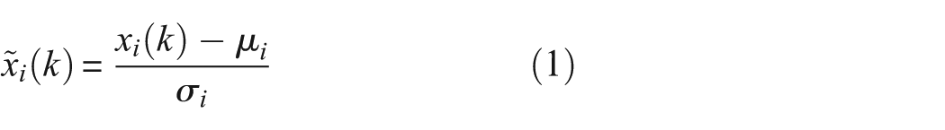
or spatial standardization
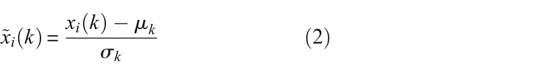
can be applied. Here,
The training process begins by encoding the high-dimensional input data
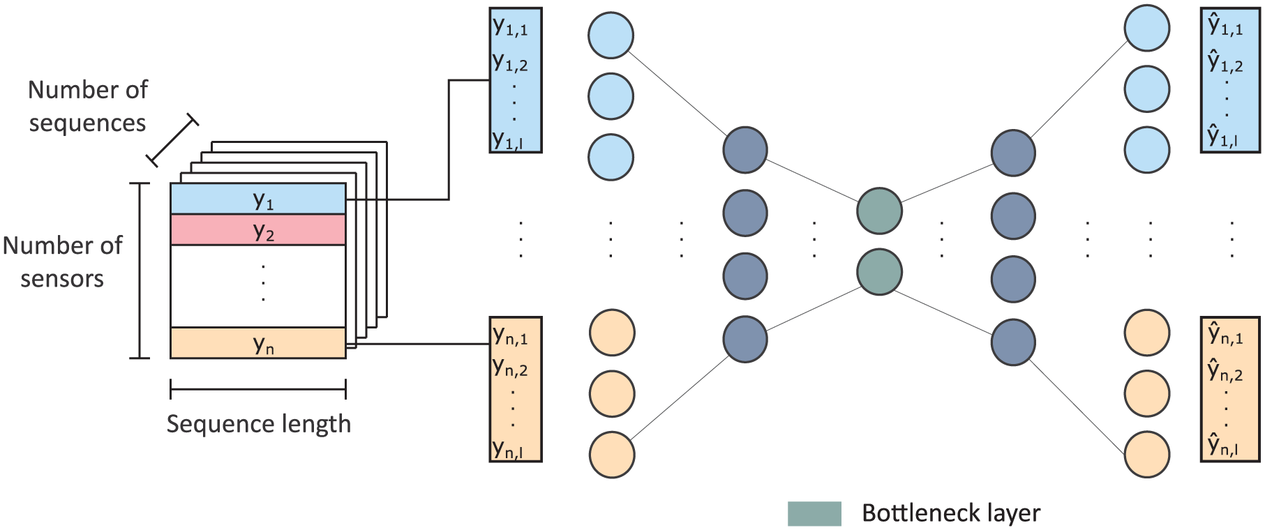
Splitting the time-domain signals into a defined sequence length (left) and how these values are fed to the encoder (right). The implemented autoencoder has a symmetrical structure and consists of at least five layers of neurons. The connections between the neurons are the parameters of the model that are adjusted in the training process to minimize the loss function.
The training involves minimizing the discrepancy between the target values
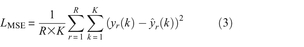
The network weights W are iteratively optimized using the first-order gradient-based optimization of stochastic objective functions called Adaptive Moment Estimation (ADAM) 53 by adjusting them according to the gradient of the loss function:
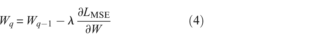
Where q is the number of iterations, and λ is the learning rate of the optimizer, which controls the step size during weight updates. The batch size is the number of samples processed before the model’s internal parameters are updated in one iteration of training. An epoch is one complete pass through the entire training data set, where the model sees each sample once.
Pearson correlation coefficient between input and residual signal for damage detection
The autoencoder’s training is conducted to reconstruct data from the healthy state accurately and to detect anomalies when a structural change (potential damage) of the system appears. To measure these changes, the difference between the target values

The residual time-domain signal is defined as:

To evaluate the residuals of the autoencoder, it comes naturally to employ its mean.
38
The mean absolute error is well-known and frequently used.
54
As the autoencoder decodes the latent space to reconstruct the original inputs, the anomaly score can be named the reconstruction error of the model. An overview of different residuals for time-domain signals when using neural networks can be found in Penner.
55
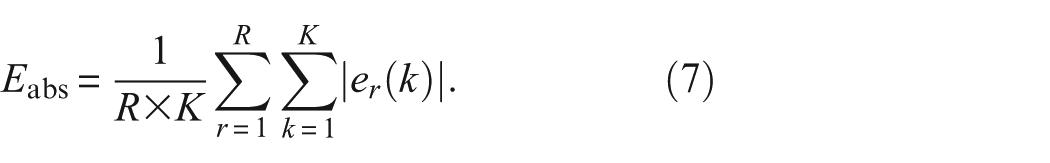
The mean absolute error averages the magnitude of errors
The attentive reader might wonder why the error metric is not the same as the previously introduced neural network’s loss function in Equation (3). Both anomaly scores are ways of measuring the reconstruction error and, consequently, are very similar. Nevertheless,
The results obtained in Römgens et al.
56
imply that the reconstruction error is a suitable parameter for distinguishing between different states when the excitation intensities are very similar. However, for real-life validation, this condition is often violated, and the excitation of the underlying system is unknown and uncontrollable. Römgens et al.
34
showed that the Pearson correlation coefficients between the inputs and the residual time-domain signals result in amplitude-related normalization and improved damage indicators. The general idea is to increase the robustness of the autoencoder’s evaluation without standardization of its inputs, as these modifications can decrease sensitivity toward damage. When the model encounters data that do not match the patterns it has learned during training, the residual time-domain signals consist heavily of repeated parts from the input signals. Consequently, the correlations between the inputs and residuals of the model are abnormally high. In contrast, a well-trained model absorbs most of the input data when evaluating the same health state. As a result, the errors mainly consist of noise highly uncorrelated with any input signals. To avoid negative values canceling out positive values, the absolute values of the Pearson correlation coefficients, namely,

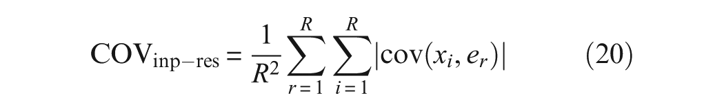
The covariances of the model’s inputs
Covariance between input and residual signal for damage localization
For data-driven damage localization in global and local SHM, the damage position can be narrowed down to adjacent sensors, assuming that the channel closest to the structural change deviates most compared to the reference state.
30
By assessing the input–residual correlations as introduced in Römgens et al.,
38
more precisely calculating the absolute covariance of the input signals
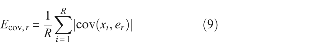
The anomaly score is further referred to as the residual covariance
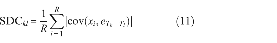
Regarding GW’s damage localization of a CFRP materials plate, it comes naturally to employ RAPID as it is well-known for visualizing the signal difference coefficient (SDC) values as proposed in Tabatabaeipour et al.
57
Notably, rather than identifying a sensor that deviates the most from the healthy state, the algorithm provides a damage position on a two-dimensional plate, for example, as illustrated in Figure 13, based on transmitter–receiver scores. Most often, the method uses Pearson correlation coefficients as the SDC values to describe the probability of damage presence between the different transmitter–receiver pairs in an ultrasonic sparse array. For each transducer pair (transducer k and receiver l), a distribution function
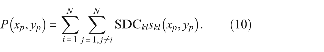
N is the total number of transducers in the sparse array. The higher the
The piezoelectric receiver’s signals are the input signals
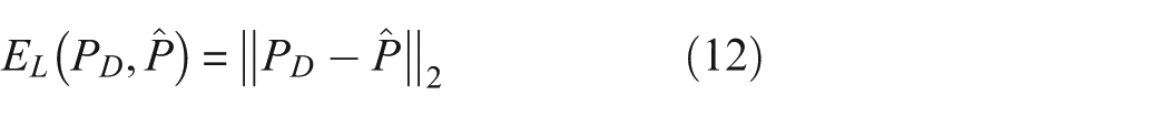
It is assumed that the transducer pair’s paths closest to the damage are associated with the highest values. Consequently, the estimated damage position
The localization error
Dimensioning of the autoencoder
Time-domain signals are acquired continuously to observe and analyze a system for monitoring. When dividing each signal into a defined number of short-term sequences, the length of the sequences l can be estimated according to Ma et al. 36
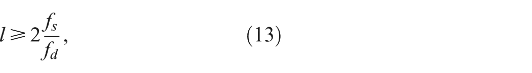
where
In this work, the lowest number of neurons is estimated by evaluating the PCA using the autoencoder’s inputs as suggested in Römgens et al. 34 It has been shown that quantifying the significance of each additional principal component for the neural architecture search can provide an excellent overview regarding the optimal bottleneck dimension. By evaluating the whiteness property, that is, the independence of the estimation errors, the ideal number of principal components can be found as an approximation for the bottleneck dimension. A good choice regarding the number of principal components has been made once the linear dependencies between the estimation errors of the learning data sets are no longer decreasing. The noise covariances are taken from a typical approach for testing the property of the whiteness test, 30 precisely the common test statistics for whiteness
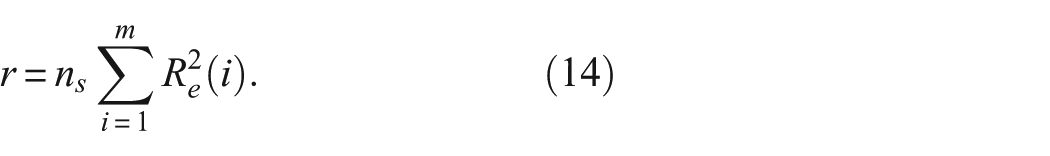
The sum of the squared correlation function
The approach is mainly driven by the assumption that the residual time-domain signals of an over-fitted or under-fitted model consist of linear dependencies, which can be quantified using the whiteness property. This results in a minimum at which the optimal number of neurons can be easily identified.
To effectively conduct temperature compensation for the autoencoder, the training phase is diversified by selecting data sets, including various temperature states. The data-driven temperature compensation accounts for the structure’s temperature-dependent varying states. This data normalization strategy does not model the dependency of the structure’s dynamics (or wave properties) and EOCs directly. Rather, the dependencies are expected to be extracted from the baseline data.
As the number of neurons in the bottleneck dimension has been defined, the model’s hyperparameters can be adjusted using Bayesian optimization. Early stopping is a regularization technique that involves halting the training process once the model’s performance on a validation set stops improving to prevent overfitting. The combination of highly informative input data and a substantial number of training examples effectively further minimizes the risk of overfitting. Due to the sequencing of the time-domain signal, a single data set produces enough examples to adjust the weights properly. It is recommended to apply a sliding window with a stride equal to the window length. While overlapping windows could further augment the data set and help mitigate overfitting, the experiments indicated that this was unnecessary, suggesting that overfitting was not an issue.
Case study 1: vibration-based SHM
External influences such as excitation or temperature play a crucial role when monitoring the health state of engineering structures. Laboratory experiments can help to conclude the impact of these factors, but they are in many cases challenging to conduct due to the limited test facilities. The Test Centre Support Structures Hannover (TTH) offers a unique infrastructure for testing all types of support structures (towers and foundations), and also a climate chamber to simulate different weather conditions. A redesign of the cantilever beam experiment introduced by Wolniak et al. 58 has been set up inside the climate chamber to investigate the influence of temperature variation on detecting and localizing damage.
Cantilever beam in a climate chamber
The beam experiment consists of a steel cantilever beam with fishplates mounted on the structure, as shown in Figures 2 and 3. According to the figures, the fishplates can be replaced with damaged fishplates to investigate different damage scenarios. Structural damage is assumed to manifest as stiffness deviation in a specific geometric area of a structure. This work investigates damage introduced by a discrete slendering of the fishplate specimen. This locally weakens the cross-section of the fishplate. Figure 4 shows a photograph of the damaged fishplate and the undamaged state where the cross-section does not change. By replacing the original fishplate of the structure, the stiffness can be changed, and artificial damage is introduced. The steel cantilever beam is excited using a proprietary, contact-free electromagnetic shaker placed at the root of the beam. The shaker introduces broadband white-noise excitation into the structure in a range of up to 400 Hz. The structural vibrations are measured using piezoelectric acceleration sensors and recorded using a 24-bit digital data acquisition system.
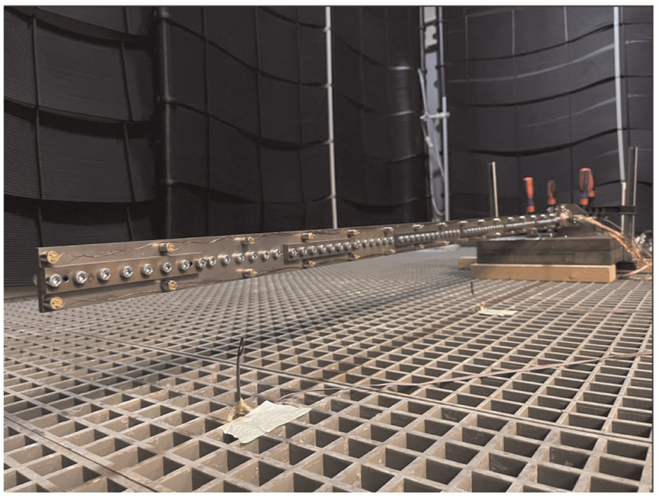
Cantilever beam in a climate chamber.
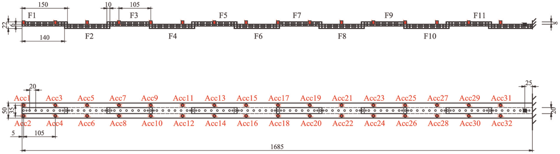
Schematic drawing of the cantilever beam positions instrumented with 32 accelerometers and 11 damage positions. For a better overview, the screws and pins are omitted in the drawing. The damage introduced by replacing fishplate F10 is analyzed using only sensors Acc1, Acc16, and Acc31.
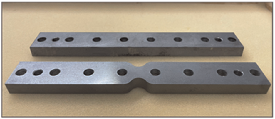
Photograph of the reference configuration (top) and the discrete damaged fishplate (bottom). The stiffness of the fishplate has been locally reduced by up to 50%, which results in only about a 0.5% reduction in the global stiffness.
The main changes to the experiment introduced by Wolniak et al. 58 are as follows:
The new steel beam is 1685 mm long and has 11 fishplates screwed on.
The number of accelerometers has increased from 16 to 32, and they are placed in two parallel lines. This setup allows us to investigate different sensor configurations.
To increase the reproducibility of the results, alignment pins for the fishplates were used, and the damaged fishplates have a controlled profile compared to saw cuts introduced by hand.
To investigate only stiffness degradation, the weight difference resulting from the slendering has been equalized by attaching magnets to the damaged fishplate instead of using fishplates that are fractions of a millimeter wider than the undamaged ones.
The main focus of the experiments is the influence of the temperature, which is controlled by regulating the ambient temperature inside the climate chamber. Three temperature sensors are placed inside the chamber to capture the variations. The temperature influences the structural stiffness of the beam, which is shown in Table 1. As illustrated in the table, the rise in temperature results in reduced stiffness, which subsequently lowers the system’s horizontal bending natural frequencies, referred to as B-x. The frequencies have been identified using Stochastic subspace identification (SSI), following the methodology established by van Overschee and De Moor.59,60 The range of temperature has been from 16°C to 40°C, more precisely 16°C, 20°C, 25°C, 30°C, 35°C, and 40°C. Each temperature has been set for at least 4 h to allow the beam structure to adapt to the increase in temperature. For the investigations in this work, only the last 10-min intervals of each temperature level are used to ensure that the structural temperature corresponds to the ambient one.
Overview of the experiments conducted.
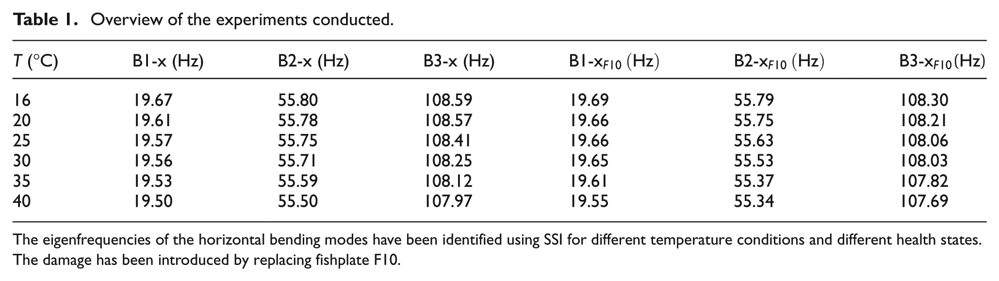
The eigenfrequencies of the horizontal bending modes have been identified using SSI for different temperature conditions and different health states. The damage has been introduced by replacing fishplate F10.
The damaged fishplate shown in Figure 4 has been exchanged with fishplate F10 on the beam experiment in closest proximity to Acc27 and Acc28. The dynamic behavior of the cantilever beam has been recorded for the above-mentioned temperatures both for the undamaged and the damaged state.
Training of the autoencoder
In this study, the autoencoder is trained on time-domain signals extracted from 3 out of 32 available accelerometers (Acc1, Acc16, and Acc31). Although a larger number of sensors is available, only a subset is used because the objective is not model updating or complete structural characterization, but rather system identification and residual-based analysis. Given the broadband nature of the white-noise excitation, it is assumed that a small number of strategically placed sensors is sufficient to capture the system’s dynamic behavior. This setup allows for investigating the influence of temperature variations on the model’s residuals without the computational burden of processing all sensor data. The training process involves defining three scenarios based exclusively on healthy conditions to explore the effectiveness of data-driven temperature compensation:
Data sets recorded at a temperature of 16°C
Data sets recorded at temperatures from 16°C to 40°C
Data sets recorded at a temperature of 16°C and 30°C
To simplify the description of the different results obtained throughout this paper, the following definitions are made:
Learning: data sets form the healthy state used during the training process to optimize the autoencoder’s weights
Validation: data sets from the healthy state not seen by the autoencoder during the training process
Testing: data sets from the damaged state not seen by the autoencoder during the training process
Precisely, for the first scenario, data sets recorded at ambient temperatures of 16°C are used for learning. In this regard, Figure 5 illustrates the influence of temperature, controlled by regulating the ambient conditions on the modal parameter B3-x of the beam. The figure shows that the increase in temperature reduces the stiffness properties and, hence, the third bending eigenfrequency of the system changes. Lower frequencies were not able to show this expected temperature dependency due to the noisy conditions in the test facility, which made the identification more uncertain. The figure implies that the correlation between temperature and B3-x can be approximated using a linear function. Furthermore, pure tracking of B3-x to detect damages at different temperatures would not be helpful without a compensation technique.
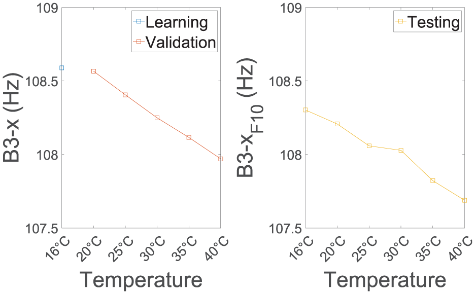
The analysis examines the average temperature of the evaluated data sets alongside the identified third bending eigenfrequency B3-x. During the learning phase, data sets from the healthy state are used to optimize the autoencoder’s weights; subsequently, validation utilizes unseen healthy state data sets, and testing employs previously unencountered data sets from the damaged state.
Given the number of input time-domain signals, the autoencoder’s neural architecture search begins with defining an appropriate sequence length l. It was determined by employing Equation (13) and computing
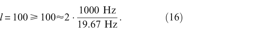
In accordance with Table 1, the fundamental (lowest) eigenfrequency has been identified from the reference state using the SSI. The original sampling rate has been kept so that time-domain signals were not changed using resampling, resulting in 6000 short-term sequences for each 10-min data set. The input dimension of the autoencoder is defined as the number of sensors times the number of the sequence length, resulting in 300 input neurons.
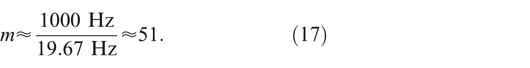
The number of neurons in the smallest layer is estimated by evaluating the test statistics for the whiteness property. Thus, the number of lags m for the estimation (see Equation (15)) can be calculated by using the sampling and the lowest measured frequency and delivers
In the present example, the test statistics for the whiteness property given in Equation (14) can be effectively applied to derive an optimal-performing architecture for the neural network. The course is not tracked as an average value over the number of principal components to recognize the effects of individual reconstructed signals and their variations. Low linear dependencies between estimation errors in the range of 35–230 principal components can be specially observed, as displayed in Figure 6. The error terms still show significant linear dependencies demonstrated by the whiteness test statistics for a number of principal components from 1 to 34. This indicates that the model struggles to reconstruct the input data or abstract the most important dynamic properties due to an insufficient number of parameters, and an under-fitting of the model. Regarding 230 or more principal components, the test statistics for whiteness property increase for a higher number of principal components, indicating an over-fitting of the model.
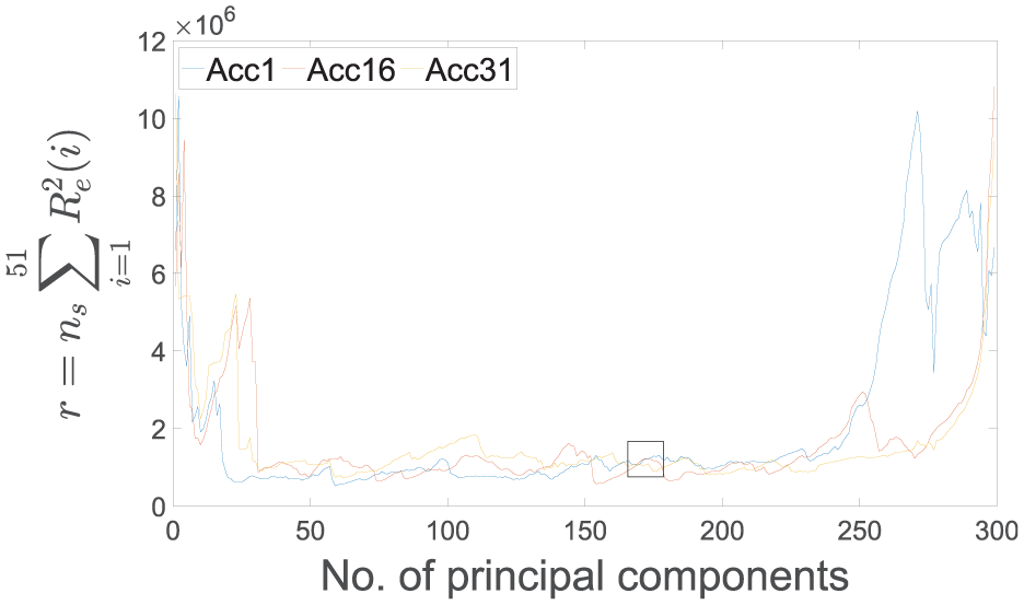
Dependence of the number of principal components on the correlatedness of the estimation errors quantified by the test statistics of whiteness property. Low values and minimal variability across different channels (Acc1, Acc16, and Acc31) of the test statistic indicate a well-performing architecture. The black box highlights the number of principal components (172) chosen based on the curves obtained.
Noteworthy, in the given example, the choice of the bottleneck dimension is not straightforward, as there is a wide range in which the model can work well. The number of bottleneck neurons is ideally quite high (150–200 neurons) to maximize the information processed by the neural network, which results in more accurate reconstruction capability. For the design of the autoencoder, a bottleneck dimension of 172 is chosen, as the test statistics across different channels show minimal variability. The results are particularly appealing due to two observations. Firstly, there is a pronounced minimum of the test statistic, making it easy to derive a well-working model. Secondly, this minimum exists without introducing a penalty function regarding the model order.
With the determination of the sequence length (300) and the bottleneck dimension of 172, the neural network’s configuration can thus be defined and the hyperparameters can be adjusted using Bayesian optimization.
61
Subject to the boundary conditions, which in the given scenario are the input and bottleneck dimension of the dimension reduction model, the other parameters such as the learning rate and the number of neurons in the encoder and decoder can be optimized concerning the validation error’s performance. The batch size is consistently defined as 64, and early stopping is applied to prevent over-fitting and improve the generalization performance. As defined earlier, the
In principle, it is obvious to use the reconstruction error of the autoencoder as a damage-sensitive feature, that is, to accumulate the absolute mean values of the residuals. However, evaluating the autoencoder’s input–residual correlations as damage indicators can be more sensitive. Moreover, for varying magnitudes of excitation, the inputs must be modified to remove the effects of different amplitudes. Typically, the input signals of the model are normalized or standardized, but this is regarded as critical, due to spatial or temporal modifications.
34
By using input–residual correlations (
Damage detection
Vibration-based SHM using autoencoders offers a robust method for detecting structural damage through raw time-domain acceleration signals. It has been observed that the damage index for data sets used during training and validation data sets at the same temperature is minimal. Consequently, each temperature level is only represented by a single file, either learning or validation data. During the damage analysis process, values for the damage indicator must be compared to some threshold, which has been derived from the damage indices of the learning and validation files. Finally, the testing data, obtained from a damaged state and unseen during training, are used to evaluate the model’s performance. Significant deviations in damage indices between the healthy and damaged states signal potential structural issues.
Figure 7 illustrates the results obtained from the training of time-domain signals at 16°C when evaluating the resulting estimation errors, or more precisely, the average magnitude of the errors (
Reconstruction error for damage detection under varying temperatures using data sets with a constant temperature of 16°C for training.
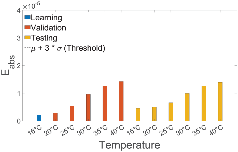
Damage detection is feasible, when training time-domain signals from 16°C to 40°C, as depicted in Figure 8. Despite this significant temperature range, the autoencoder is able to learn different states simultaneously with high accuracy. However, the reconstruction error is not perfectly constant for the healthy state, which implies that the autoencoder is reproducing the inputs rather than learning the temperature dependencies. Interestingly, the two damage indices (
Reconstruction error and input–residual correlations quantified by the Pearson coefficient for detecting the replacement of a fishplate specimen under varying temperatures. All files corresponding to temperatures of 16°C to 40°C are used during training for temperature compensation.
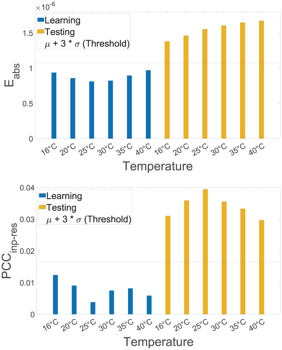
The results obtained when training the autoencoder using data sets recorded at 16°C and 30°C while evaluating the
Reconstruction error and input–residual correlations quantified by the Pearson coefficient for detecting the replacement of a fishplate specimen under varying temperatures. All files corresponding to temperatures of 16°C and 30°C are used during training for temperature compensation.
Damage localization
The five levels of damage identification increase in difficulty, and each subsequent level requires the results of the previous one. The damage localization is performed after damage has been successfully detected using the same residuals of the model. However, for a deeper understanding of the autoencoder’s performance, all data sets from the damaged state—Data sets No. 7 to 12 (Testing) from the previous figures—are analyzed for damage localization. For example, the autoencoder’s residuals, when training time-domain signals at 16°C (cf. Figure 7), are examined for damage localization, although all damage indices were below the threshold. Each sensor position’s anomaly score is extracted from the residuals using the input–residual correlation quantified by the covariance, more precisely the residual covariance. As described earlier, the data normalization strategy depends on the variation of the external factor during training, which is the temperature here. For damage localization, sensors are compared with each other to narrow down the damage position to adjacent sensors within a period, in which the system can be assumed to be stationary and time-invariant. To simplify the comparison of the residual covariances
Changing temperatures are affecting the outcome of the damage localization as shown in Figure 10. As before, the first scenario has been using time-domain signals at 16°C, more precisely, no temperature compensation has been carried out. Although the residual covariance is in most cases highest at sensor Acc31, which is closest to the discrete damage, the results obtained are not convincing. The damage position indicator varies, especially when evaluating data sets recorded at 25°C and 30°C.
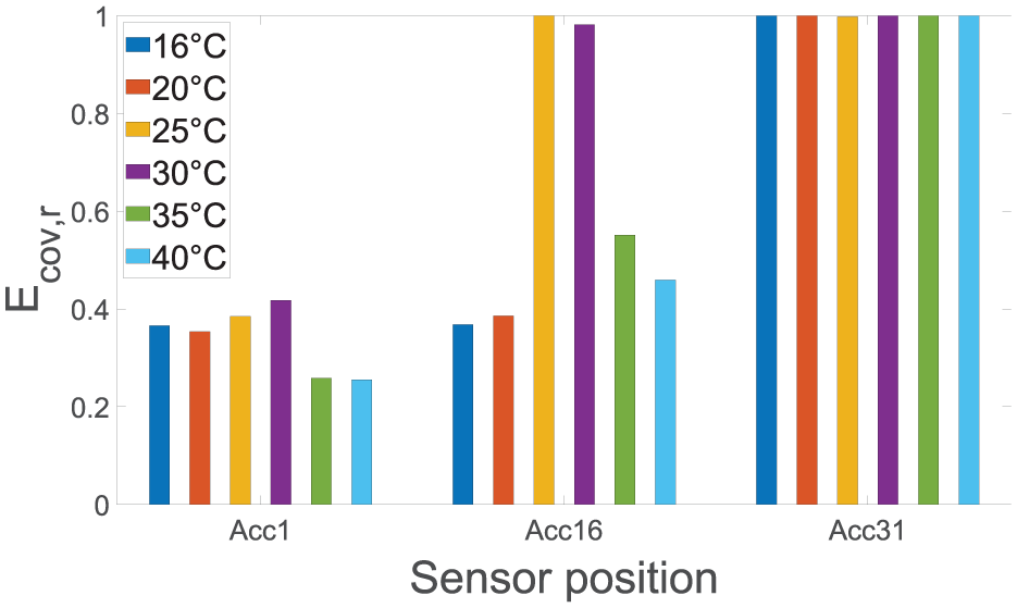
Residual covariance for damage localization under varying temperatures using data sets with a constant temperature of 16°C for training. The actual damage is in the closest proximity to Acc31.
To account for temperature-dependent varying states of the structure, the autoencoder is trained using the data sets from all temperatures. Consequently, the damage localization improves significantly, as depicted in Figure 11, showcasing the effective temperature compensation. However, as seen before, the autoencoder seemingly tries to reproduce the learned temperature conditions rather than abstracting the dependency between the dynamic properties and the temperature. It is still possible to localize the damage for all temperatures with some temperature-dependent variations in the damage position indicator.
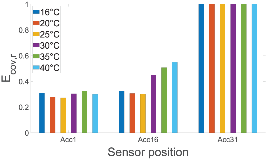
Residual covariance for damage localization under varying temperatures using all data sets for training. The actual damage is in the closest proximity to Acc31.
Consistent with previous observations, the best results are obtained when learning the 16°C and 30°C temperature states as shown in Figure 12. The residual covariance exhibits the highest values for Acc31. Additionally, the damage position indicator features a comparatively small variance for all data sets evaluated showing robustness toward varying temperature conditions. The residual covariance values generally decrease as we move away from the induced damage. In the given case, due to the sparse number of sensors, the residual covariances are very low (0.2) for sensor positions Acc1 and Acc16.
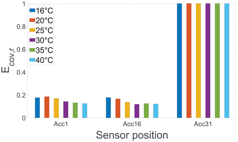
Residual covariance for damage localization under varying temperatures using data sets with constant temperatures of 16°C and 30°C for training. The actual damage is in the closest proximity to Acc31.
Discussion
The presented investigations show that the implicit system identification and the data-driven temperature compensation are practically applicable to properly capture the underlying system’s dynamic properties. This data normalization strategy is appealing since the physical information of temperature does not need to be explicitly modeled. It has been demonstrated that stiffness alterations caused by an increase in temperature significantly influence the autoencoder’s residuals. These relations are depicted in Figure 7), which shows the need for a temperature compensation procedure. The observed increase in the damage index is consistent with earlier investigations, which demonstrated a clear correlation with damage size and confirmed that even minor, practically relevant damage could be reliably detected. 56
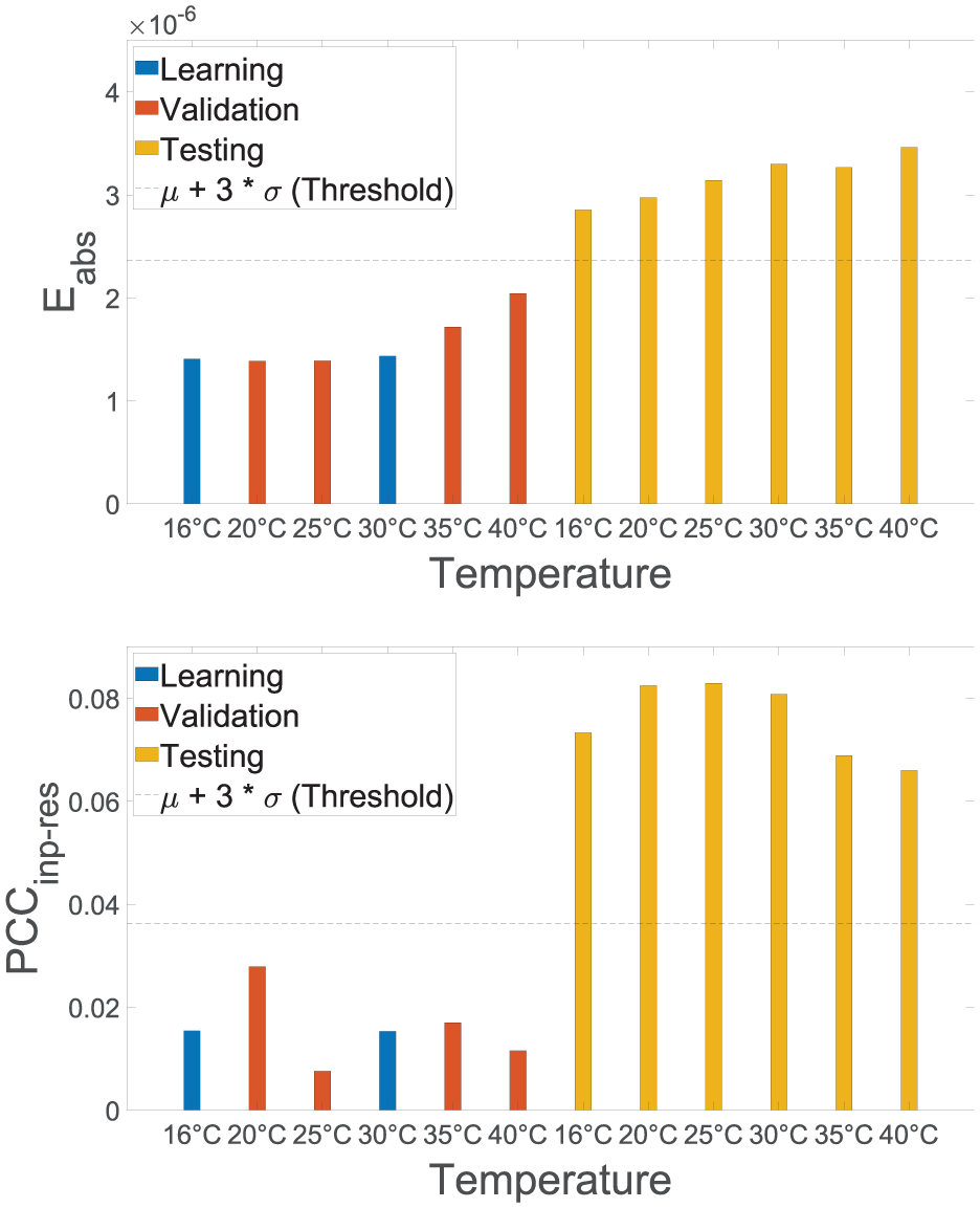
It can be derived that the damage index is perfectly constant when the temperature-dependent variance is given by two different temperature conditions. This implies that the autoencoder is learning the temperature dependencies rather than reproducing the learned inputs for different temperature conditions, see Figure 9. A possible explanation for that could be found in the linear dependencies between the temperature and the eigenfrequencies of the system as illustrated in Figure 5. It is worth noting that the models trained on data sets recorded at 16°C and 40°C yield a perfectly constant damage index. However, since these cases do not allow for evaluating extrapolation capabilities, they are not illustrated in this work. Accordingly, the neural network could map linear dependencies from external factors very easily, as only two states would be required. The temperature range can also be extended, depending on data availability, to capture larger variations such as those below 16°C or above 40°C. Given the observed extrapolation capabilities, a deviation of up to 10°C can still be tolerated, although the resulting accuracy is reduced compared to interpolated states. Note that the input–residual correlations quantified by a Pearson coefficient are throughout more sensitive toward the damage, resulting in better differentiation of both states for damage detection. Furthermore, the results presented before suggest that the localization is less affected by the temperature variations than the damage index for detection. Most probably, the eigenfrequencies are evident for damage detection in this regard, which change due to the increase in temperature. In contrast, for damage localization, the less temperature-sensitive amplitude dependencies are upmost important to narrow down the position of the damage.
In summary, for autoencoders with short-term sequences of raw time-domain signals, a data-driven temperature compensation can be carried out by maximizing the variance of the external factor. No additional interpolation scheme must be applied and even states not captured in the temperature range (red bars at 35°C and 40°C in Figure 9) can be properly extrapolated. The input–residual correlations quantified by a Pearson coefficient demonstrated throughout higher sensitivity toward damage, resulting in better differentiation of both states for damage detection.
Case study 2: local monitoring using GWs
Previously, the investigations focused on damage detection and localization under varying temperatures in vibration-based SHM. This showed that the implicit system identification can be applied in such a way that external factors, for example, temperature can be perfectly compensated when given two temperature conditions. Strongly involved in obtaining such good results have been the input–residual correlations (
Open guided waves
The time-domain signals with an excitation signal of 40 kHz, a 5-cycle Hann-filtered sine wave, provided by Moll et al.
63
are used to evaluate the previously introduced implicit system identification. The data contain several measurements taken on a CFRP
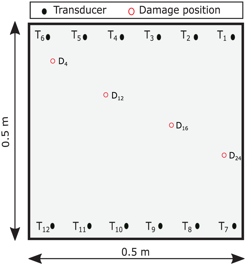
Geometry of the monitored plate with transducer positions
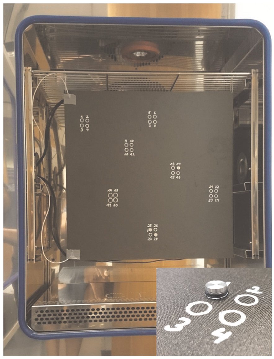
Picture of the reversible damage model in the form of an aluminum disk with a 10 mm diameter, which is placed on the composite plate in the climate chamber. 62
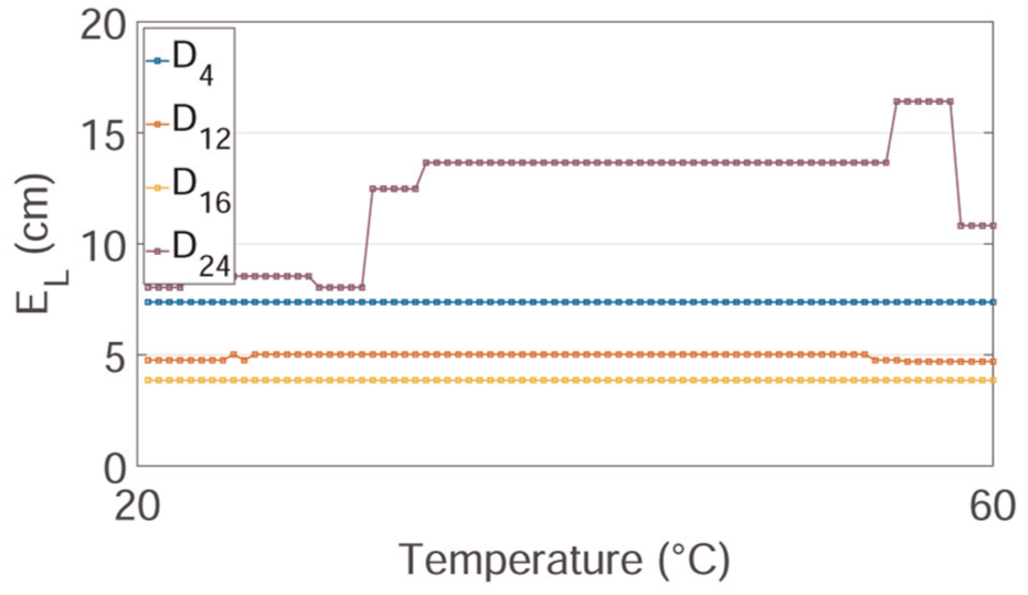
The measurements are taken both on the intact structure (the aluminum disk is not placed on the plate) and with the damaged structure (the aluminum disk is placed in different locations). Although this reversible damage model simplifies the geometry of actual delamination by focusing on changes in the structure’s mass, its interaction with guided waves similarly affects specific characteristics, such as alterations in time-of-flight and decreases in amplitude.63,64 Delamination is a critical failure mode in fiber-reinforced composites. It can directly lead to through-thickness failure due to interlaminar stresses caused by out-of-plane loading, curved or tapered geometry, or discontinuities caused by cracks, ply drops, or free edges. 64 To investigate the effects of temperature, a variation of the temperature from 20°C up to 60°C with a constant 50% RH (relative humidity) is used, as shown in Figure 15. For each damage position, 161 data sets are recorded. It has been shown that the effects of temperature significantly influence the wave’s signal and are therefore difficult to handle. 15
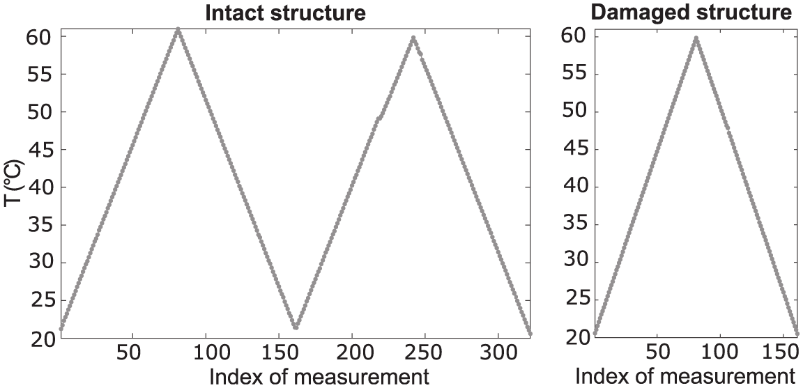
Temperature curve for the intact and damaged structure. 63 Data sets S1 to S322 are from the intact structure, and 161 data sets are from the damaged structure for each damage location.
Training of the autoencoder
To effectively train an autoencoder for different temperature conditions on GWs, it is necessary to diversify the training data and use data sets that include input data corresponding to various temperature states. The neural network learns to encode the input data in a way that captures the underlying patterns or features associated with different temperature conditions. Following proper compensation, it is assumed that the residuals produced by the autoencoder are effectively decoupled from temperature effects and can thus serve as reliable indicators for damage analysis. As described earlier, a total number of 322 data sets (S = set) is measured for the intact state, and the temperatures are varied resulting in two temperature cycles (cf. Figure 15). Three different scenarios are chosen to investigate the temperature influences during the training process:
Only data sets recorded at a temperature of 20°C (S1, S160, and S320).
Data sets recorded at temperatures from 20°C to 60°C (S1, S10, S20, …, and S320).
Data sets recorded at a temperature of 20°C and 60°C (S1, S80, S160, S240, and S320).
The fundamental frequency can be used to estimate the minimum sequence length as defined in Equation (18). To increase the probability that the frequencies are excited in each sequence of the real structure, a longer sequence length is selected based on the criterion as follows:
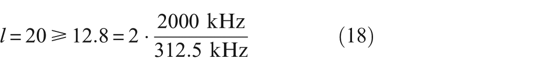
With a total of 13,108 samples, each signal is segmented into 131 short-term sequences. Noteworthy, the equation is based on natural frequencies. However, in the given context, it is used to estimate the sequence length. The fundamental frequency has been chosen in regard to the reflected waves, which have a basic frequency of 312.5 Hz.
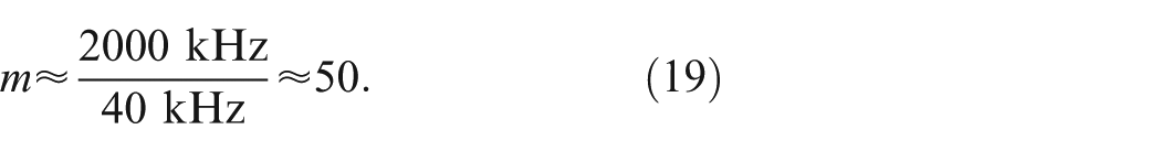
The bottleneck dimension is estimated using the whiteness property of the model’s estimation errors. As described earlier, it is helpful to try out every possible configuration to make it easier to decide which dimension reduction provides a good model; calculating all possible bottleneck dimensions for the neural networks would be disproportionate to its benefit. Hence, due to its simplicity and low computational time, the PCA is used instead of the autoencoder’s repeated training across various bottleneck dimensions to approximate the reconstruction of the signals and find the optimal parameter. Thus, to determine the number of neurons in the smallest layer, the PCA based on the whiteness property is used. To estimate the number of lags for the whiteness property, Equation (15) is utilized
As previously indicated, the optimal number of principal components can be identified to approximate the autoencoder’s bottleneck dimension. To facilitate better differentiation, this analysis focuses on 8 out of the 66 transducer pair signals. Consistent with the vibration signals shown in Figure 6, a significant linear dependency is observed within the residual time-domain signals when using a small number of principal components, which indicates under-fitting of the model, as depicted in Figure 16. The analysis suggests that within the range of 250–700, the errors primarily consist of highly uncorrelated noise components. These observations closely resemble those found in vibration-based SHM, indicating that the whiteness property effectively informs the estimation of the autoencoder’s architecture when assessing UGWs. Based on the low-test statistic values and their minimal variability across different channels, it is concluded that configuring the smallest layer with 400 neurons results in an optimal performance of the deep neural network’s architecture.
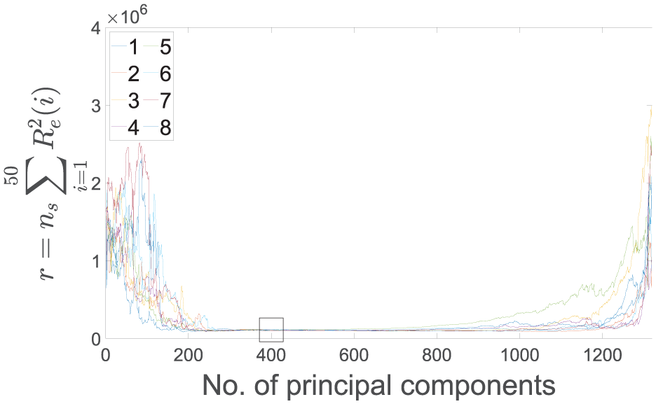
Dependence of the number of principal components on the correlatedness of the estimation errors quantified by the test statistics of whiteness property. Low values and minimal variability across different channels (66 transducer pair signals) of the test statistic indicate a well-performing architecture. The black box highlights the number of principal components (400) chosen based on the curves obtained. Only 8 of the total 66 transducer pair signals are included in this chart for the sake of clarity.
Damage detection
For damage detection, the residuals of the trained autoencoder are analyzed, and two damage indices are compared to validate the methodology applied. Each data set is evaluated using the autoencoders’ residuals by comparing their mean and the input–residual correlation quantified by a Pearson coefficient. In both cases, the evaluations result in a single anomaly score for every data set, specifically 131 short-term sequences. The absolute value of each input–residual correlation (see Equation (8)) prevents negative and positive values from equalizing each other as described earlier. Thereby, the maximum value of the anomaly score does not exceed 1, and the lowest possible value is 0.
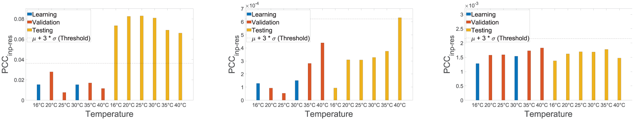
Figure 17 illustrates two damage indices—the reconstruction error of the autoencoder and the averaged input–residual Pearson correlation coefficients—when evaluating data sets of the intact structure. The figure consists of bars, each visualizing the autoencoder’s anomaly score. A dashed yellow line is added to highlight the temperature variations consistent with Figure 15. As described earlier, the blue bars highlight the anomaly score of data sets used for training the autoencoder. The scores detect the changes in time-domain signals mainly linked to the temperature variations, as the autoencoder has only been trained on S1, S160, and S320 acquired at the same temperature (20°C). Obviously, this is not ideal for damage detection, but it shows that the autoencoder can effectively reproduce these temperature variations.
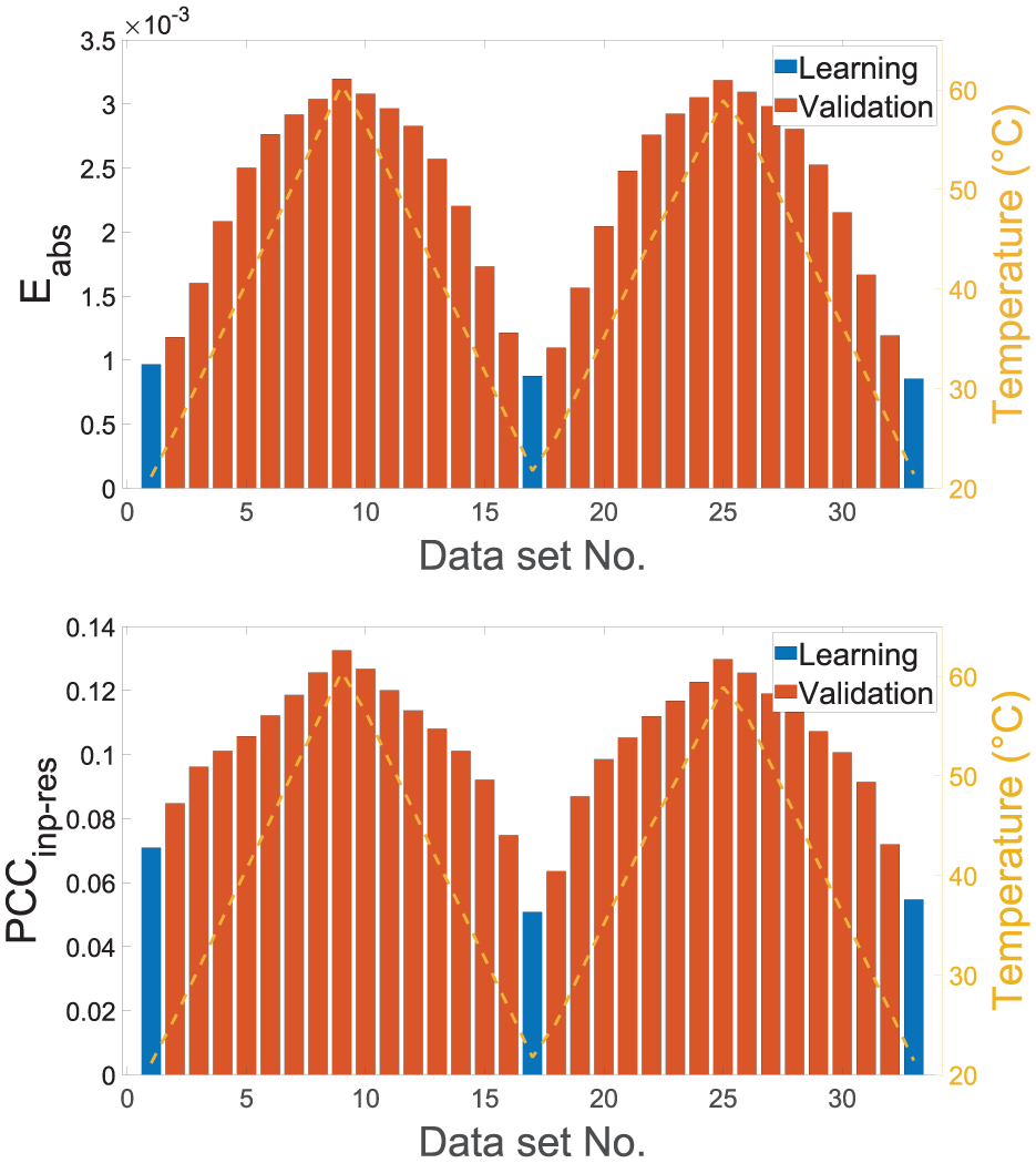
Reconstruction error and input–residual correlation under varying temperatures when evaluating all data sets from the healthy state. Only temperatures of 20°C are used for the training process.
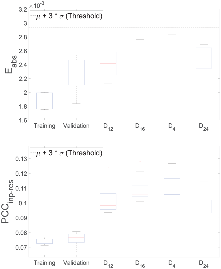
A more precise understanding of the results and evaluation of the model can be achieved, if the data sets of the damaged state are included, see Figure 18. The autoencoder has also been retrained to demonstrate the reproducibility of the autoencoder’s training. The figure shows the boxplots of two damage indices extracted from the autoencoder’s residuals when evaluating the damage positions
Reconstruction error and input–residual correlation for detecting
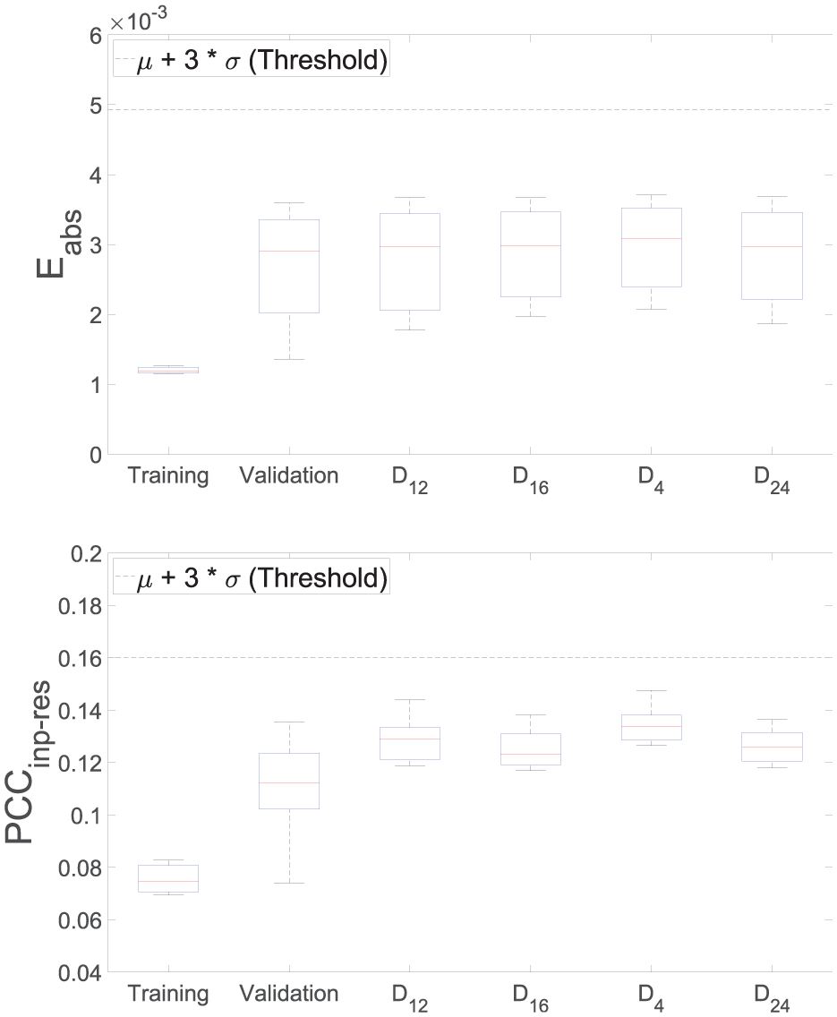
The findings pertaining to the training of temperatures from 20°C to 60°C are depicted in Figure 19. The presentation style of the damage analysis results is identical to the one used before. Given these results, it can be observed that, despite the temperature variations, damage detection is successful for all four damage positions, and both damage indices. As before, the input–residual correlations enable a better distinction between healthy and damaged conditions to be made. The greatest deviations from the reference state can be seen in position
Reconstruction error and input–residual correlation for detecting
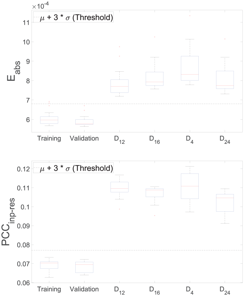
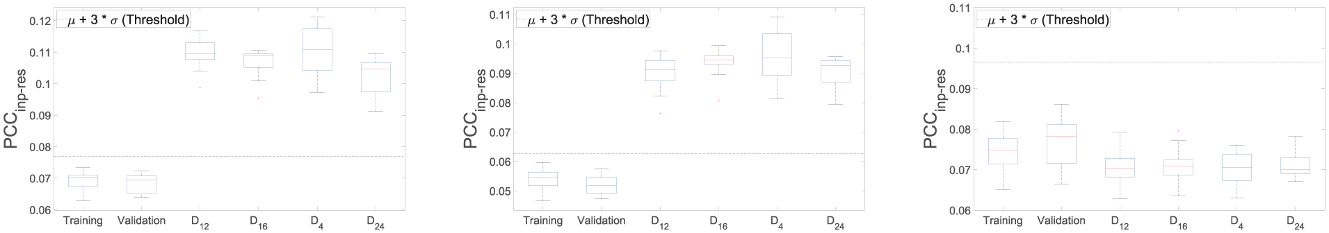
Regarding the final results in Figure 20, where only temperature states of 20°C and 60°C were used for training, the damage detection is not feasible, when evaluating the reconstruction error of the autoencoder. Although the damage-sensitive feature tends to be higher for the four damage positions compared to the healthy state, a differentiation is hardly possible. On the contrary, if the residuals of the same model are evaluated using the input–residual correlations, more precisely
Reconstruction error and input–residual correlation for detecting
Damage localization
To best evaluate the capabilities of the data-driven model, it is necessary to derive a damage position in two-dimensional coordinates from the model’s residuals. For this purpose, the SDC values of the RAPID are described by the residual covariances of the autoencoder. Consequently, the higher the residual covariance of the sensor, the higher the associated path is weighted. From this, the position on the plate with the highest probability of damage is determined and the Euclidean distance
Table 2 gives an overview of the localization results obtained. Consistent with the training for damage detection, three training scenarios have been investigated. As expected, the localization error is highest when the temperature dependence is not given to the model by using different temperature conditions. Most interesting, the autoencoder can transfer particularly damage-sensitive features with the RAPID, so that the localization has a comparatively low error, as shown for the second and third scenarios.
Comparison of damage localization results using the autoencoder’s input–residual correlations as SDC values for RAPID.
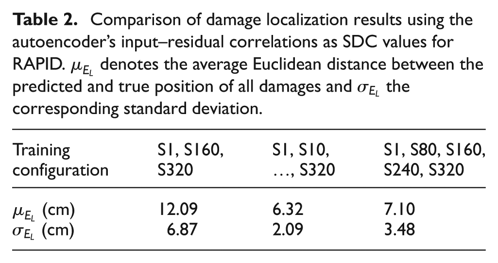
Figure 21 highlights the effects of temperatures on the localization outcomes. The model has been trained on data sets recorded at 20°C. As described earlier in Figure 15, the temperature increases from 20 to 60°C and decreases again resulting in 161 data sets for each damage scenario. For similar temperatures, the localization error is quite low as illustrated in the figure. However, in areas where the autoencoder has no training data, the results significantly worsen. Although these results were expected to be obtained, the outcomes increase the trustworthiness of the results. Due to the replacement of the SDC values by the autoencoder’s residual covariances and then visualization by using the RAPID, uncertainties are introduced. Due to the parallel arrangement of sensors, the damage positions
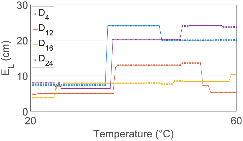
Localization error
Figure 22 highlights that the autoencoder is capable of simultaneously mapping different states. As mentioned earlier, 33 data sets associated with temperatures ranging from 20°C to 60°C have been used in the training process. It is evident that the autoencoder successfully compensates for temperature effects as the localization error does not change. Despite the partially nonlinear influence of temperature on the behavior wavelength and wave velocity, robustness toward different temperature conditions is achieved without a comprehensive representation of all temperatures. However,
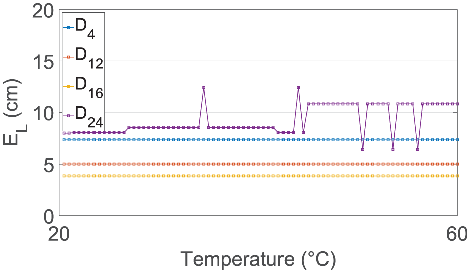
Localization error
Figure 23 shows similarities to the results of the vibration-based SHM (cf. Figure 9). It is possible to cover the temperature range in such a way that the influencing variables can be compensated for by the choice of learning files. For training, five data sets have been chosen, which were recorded during the maximal and minimal temperatures of the experiment. The SDC values which are given to RAPID in order to visualize the most probable damage position are derived from the autoencoder’s residuals. Due to the slight changes observed in the figure, it is evident that despite the large temperature range, the residuals of the autoencoder almost do not change. This indicates, as shown before, that the effects of temperature can be neglected, or more precisely, significantly reduced. This is particularly interesting because the influence of temperature on the wave velocity is nonlinear. Nevertheless, it cannot be ruled out that the nonlinear influence is well approximated by a linear function and that problems arise if these nonlinearities are more prominent. Overall, it should be noted that it is not only possible to compensate for the variations in ambient conditions but also to teach the autoencoder maximum and minimum temperatures. In this case, two learning files would probably have been sufficient, but due to the small amount of data, a total of five files have been used.
Localization error
Discussion
The presented investigations show that the autoencoder is capable of learning the properties of GWs for implicit system identification. The autoencoder’s residuals correctly change due to temperature variations as illustrated in Figure 17. By training 33 of 322 data sets, the autoencoder was able to compensate for these effects in a data-driven manner, cf. Figure 19. Damage position
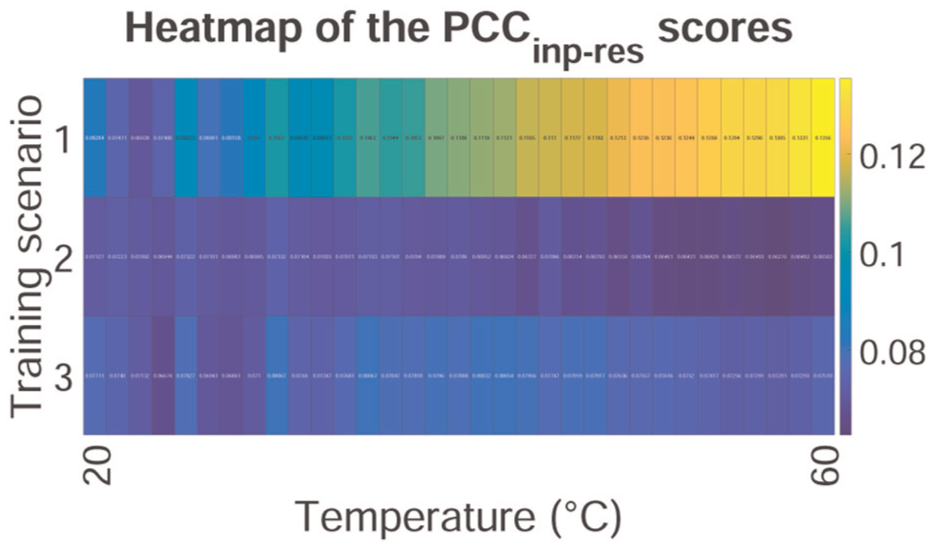
Illustration of the remaining temperature dependencies for each training scenario. Low variations of the anomaly score indicate that the model has abstracted the temperature dependencies.
For damage localization, the autoencoder’s residual covariances have replaced the SDC values of the RAPID to derive a damage position on the two-dimensional plate. When training only data sets recorded at 20°C, the necessity of temperature compensation has been made visible in Figure 21 as the localization error scatters due to temperature variations. However, the suitability of autoencoders to localize the damage positions is already visible in the figure as the localization error is very small in the learned temperature range (20°C). Figure 22 illustrates that data sets from 20°C to 60°C in training can compensate for the temperature effects effectively. The constant values of the localization error imply an autoencoder in which the residuals of the model are not affected by the temperature variations. When using two temperature conditions during training, it was also possible to compensate for the temperature effects as shown in Figure 23. As before, due to the limited information regarding the temperature variations, the results have been slightly worse than the second scenario. Noteworthy,
Comparison of case study 1 and 2
In general, vibration-based and GW-SHM have very few points of overlap. Vibration-based methods have in common that a structural change due to damage results in a more or less pronounced change of the physically interpretable dynamic properties. In GWs, the change of artificial waves that are susceptible to structural and material interferences caused by damages, defects, and boundary edges are analyzed. In this regard, model-based methods play virtually no role due to the complex environment. However, both systems can be monitored with data-driven models using time-domain signals for unsupervised SHM. As shown in Table 3, the main differences are the UGWs in comparison to naturally occurring vibrations resulting in very different sampling frequencies and signal lengths.
Overview case study 1 and 2.
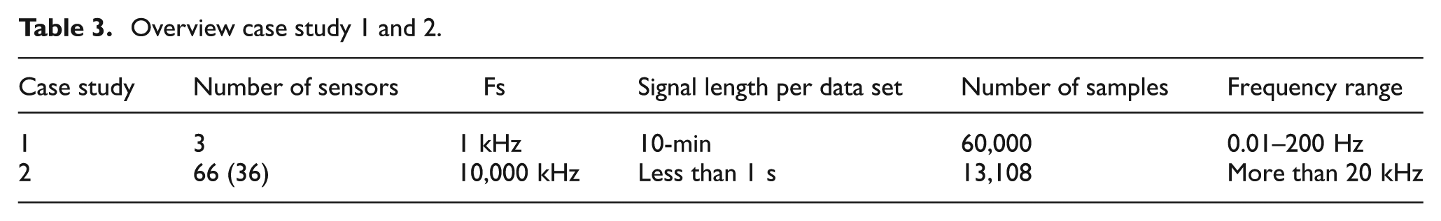
For both case studies, autoencoders with sequences of raw time-domain signals have shown their suitability for damage detection and localization under varying temperature conditions. The sequence length has been estimated using the fundamental eigenfrequency and in regard to the reflected waves of the active monitoring system. The autoencoder was further dimensioned using the whiteness property by evaluating the PCA residuals, which showed similar curves despite the differences in signal characteristics. The autoencoder’s evaluation using input–residual correlations quantified by a Pearson correlation coefficient was not only transferable to GWs, but the impact was even more significant. It is assumed that the correlations can be quantified even better due to the simple signal characteristics of GWs. In vibration-based SHM, the temperature compensation has been more effective when using two temperature conditions only. Assumingly, the autoencoder rather learns the linear temperature dependence on the vibration signals and is not focused on each data set individually (over-fitting), resulting in improved damage detection. On the contrary, in GW-SHM, the temperature compensation has been due to the nonlinearities more effective when using several conditions of the external factor. However, it is possible to obtain quite good results when training data sets from two conditions, more precisely 20°C and 60°C. As for the cases considered in this paper, the approach is a potent tool in vibration-based SHM (passive) and GWs-SHM (active).
We consider changes made to the time-domain signals to be critical, as information can be changed or lost. To elaborate on that, the impact of standardization is discussed in both case studies for damage detection and localization under temperature variations. Additional findings such as the adaptation of the loss function can be conducted to regularize the autoencoder’s training effectively. The changes made to the loss function are not crucial but can improve the performance of the network.
Modification of the raw input signals
Figure 25 illustrates the damage detection results obtained for the first case study when using raw time-domain signals, temporal (cf. Equation (1)), and spatial (cf. Equation (2)) standardization. In vibration-based SHM, the impact of standardization on raw time-domain signals can be explained from a physical point of view. When temporal standardizing is applied, the original amplitude dependencies between sensory is lost, but the eigenfrequencies remain the same. As a result, the performance of damage detection is reduced, but for some temperatures, for example, 20°C and 25°C, damage detection would still be possible when using a different threshold. For spatial standardization, the eigenfrequencies of the system are changed, and only the amplitude dependencies of the dynamic system are kept. As the eigenfrequencies are crucial for detecting the presence of damage, this would have failed as illustrated in Figure 25.
Input–residual correlation for detecting the discrete damage under varying temperatures in the climate chamber. The raw time-domain signals (left), temporal (mid), and spatial standardized (right) signals are fed to the autoencoder as input.
In GWs for damage identification, it has also been observed that the damage sensitivity is reduced due to the modification of the input signals. To substantiate the findings of the evaluations, a direct comparison is made between standardization and the input of raw data. Figure 26 shows that temporal standardization does not considerably influence the results. Due to the standardization of the model’s inputs, the performance of unseen data during training from the healthy state has a very similar performance. A good separation of the learning data and the data after applying the additional mass is possible. However, for spatial standardization of the model’s inputs, the detectability is completely lost. As the amplitude dependencies are not relevant for damage detection, standardization has no influence on the results. On the other hand, only using the amplitude dependencies makes it impossible to detect damage.
Input–residual correlations for detecting
Table 4 summarizes these findings regarding short-term sequences from time-domain signals as the input for the autoencoder and also shows the impact on the damage localization results. For damage localization in vibration-based SHM, spatial standardization is less crucial than temporal standardization, as eigenfrequencies play a subordination role and the amplitude dependencies are more important to maintain. However, when standardizing the signals in the time-domain, the original amplitude dependencies are lost, and localization is not possible anymore. For GWs, as described above, spatial standardization results in amplitude dependencies being fed to the autoencoder, which is not helpful for damage detection or localization. Standardization in the time-domain results in slightly higher damage localization errors. In summary, standardization is especially critical in vibration-based SHM as changes are made to the time-domain signals of the system, which consists of the naturally occurring vibrations. For GWs, the standardization does not have the same impact but slightly worse results are obtained for damage localization, more precisely a higher localization error.
Influence of modifying raw signals in active and passive SHM for the method proposed.
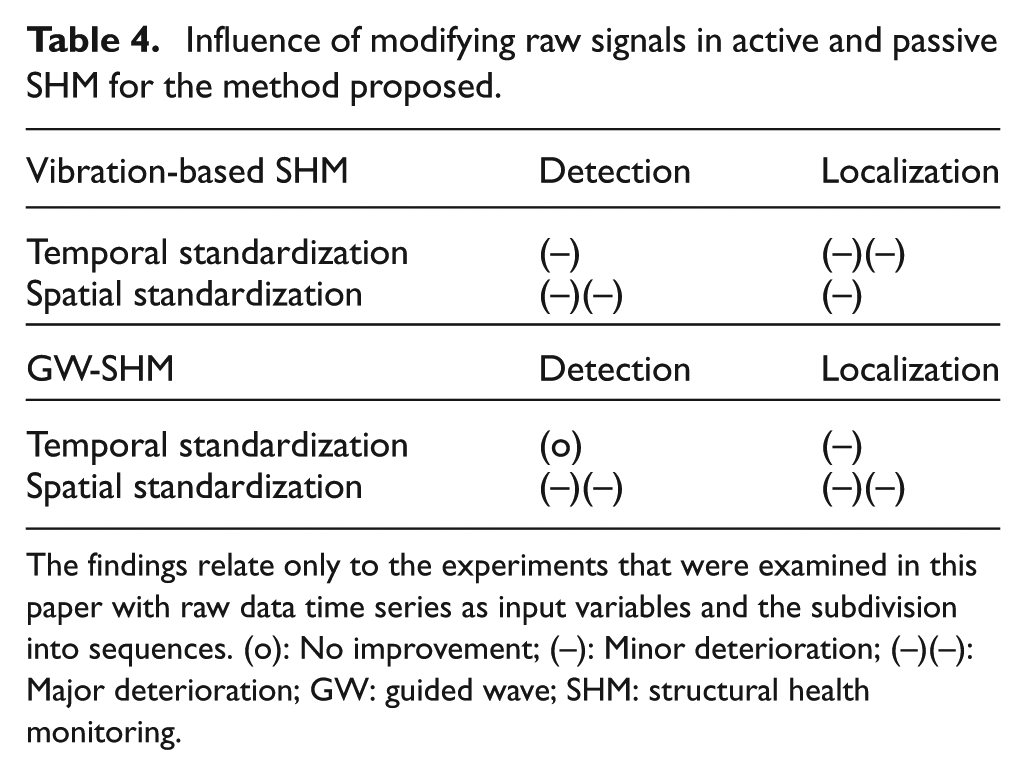
The findings relate only to the experiments that were examined in this paper with raw data time series as input variables and the subdivision into sequences. (o): No improvement; (–): Minor deterioration; (–)(–): Major deterioration; GW: guided wave; SHM: structural health monitoring.
Amplitude-related normalization regarding vibration-based SHM and GWs
It was derived that for damage detection, an amplitude-related normalization is inevitable due to the different excitation intensities in real-life. 34 In this paper, the signals have been similar for both studies in such a way that amplitude-related normalization is not needed. However, the input–residual correlations quantified by a Pearson coefficient have been used to show its applicability also in this regard. Noteworthy, the use of the input–residual correlations can be adapted to exclude the amplitude-related normalization, more precisely, the standard deviations:
This can lead to a better evaluation of the autoencoder’s residuals as these are more representative. As discussed earlier, the modification of inputs is seen as critical and therefore the input–residual correlations were applied, because no changes to the inputs of the model have to be made. In general, this has shown to be very effective, but there could be different metrics, such as mutual information, which also takes nonlinearities into account.
Regularization of the autoencoder’s training
The training of the autoencoder is crucial, as the performance and applicability of the autoencoder largely depend on how well it has been optimized. Generally, the loss function of the neural network
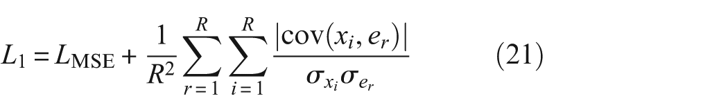
Therein,
Conclusion
Within this work, we investigated an autoencoder with short-term sequences of raw time-domain signals for unsupervised damage detection and localization under varying temperatures in vibration-based SHM (case study 1) and GWs-SHM (case study 2). To elaborate on that, the laboratory experiment of a dynamically excited modular steel cantilever beam with manually controllable ambient temperatures in a climate chamber is presented in detail. The data normalization strategy consists of temperature dependencies that are extracted from the baseline data, rather than modeling the dependencies independently. It has been shown that the data-driven model can perfectly abstract the dependency when two temperature conditions are given to the model, allowing for robust damage detection and localization. This concept remains applicable for even larger temperature variations. Further, the same methodical approach has been applied to an active monitoring system, precisely the OGW data set. Crucially, the transfer from structural dynamics to evaluating wave propagation properties has been successful, and plausible results have been obtained. Applying input–residual correlations quantified by a Pearson coefficient to evaluate the autoencoder’s performance provides a very valuable damage indicator as the signal characteristics of GWs are less complex. Contrary to the first case study, the autoencoder performed best when several different temperature conditions were trained for data-driven compensation, which resulted in a smaller localization error from 12.09 to 6.23 cm. Furthermore, a good approximation (7.10 cm) has been demonstrated when using only two temperature conditions. This instance can be explained by the more complex temperature influence on GWs affecting properties such as speed, amplitude, and wavelength. A negative impact of standardization has been observed in both case studies, mainly due to the changes made to the signal characteristics. The proposed approach is inherently data-driven, with its limits closely tied to the availability and representativeness of the training data sets. Challenges may arise when global monitoring techniques on large-scale structures lack the required sensitivity (minor damages) or the environmental influences make diagnostics unreliable. In summary, the proposed method for implicit system identification is applicable in vibration-based and GWs-SHM, or more generally speaking: in active and passive SHM. The use of these models promises to be a robust and sensitive tool for damage detection and localization under varying temperature conditions. Finally, the investigations show that the data-driven temperature compensation depends on the external factor’s complexity, linear dependencies such as temperature can be removed from the residuals using two temperature conditions.
Due to the results achieved with the autoencoder, the methodology can be expected to be applicable to all possible time-domain signals for implicit system identification. The extension to significantly nonlinear systems does not appear to be particularly challenging and would constitute an exciting research objective. Furthermore, integrating multimodal sensor data, such as combining guided wave measurements with vibration, strain, or environmental monitoring, could provide a more comprehensive and robust perspective on structural health.
Footnotes
Declaration of conflicting interests
The authors declared no potential conflicts of interest with respect to the research, authorship, and/or publication of this article.
Funding
The authors disclosed receipt of the following financial support for the research, authorship, and/or publication of this article: The authors greatly acknowledge the financial support provided by the Federal Ministry for Economic Affairs and Climate Action of the Federal Republic of Germany within the framework of the collaborative research project SMARTower (FKZ 03EE2041C). We also gratefully acknowledge the financial support of the German Research Foundation (Deutsche Forschungsgemeinschaft, DFG) [SFB-1463-434502799].