Influence line theory supported single sensor-based strain feature for bridge defect diagnosis

Abstract

This study established a theoretical foundation for single-sensor-based M-value feature derived from field bridge strain responses. Its ability to detect bridge structural damage was validated and explained through the influence line theories. More importantly, the variations of such a feature were further connected to the shifts of neutral axis (NA) positions. By correlating the NA position with the cracking depth of the section, the application of a single-sensor-based M-value feature was innovatively expanded to quantify bridge minor defects, such as small cracks within the section, where a design value for intact structures was proposed, offering a benchmark for quantitative bridge condition assessment and guidance for practical bridge management. A case study involving a two-span continuous bridge demonstrates the practical application of the developed feature in scenarios that lack original design information of bridge sections.

Introduction

The influence line (IL) is a crucial parameter in bridge structures, encapsulating both the mechanical and static characteristics of the system. It records the response at a given point on the structure as a unit load travels across the bridge, providing valuable insight into displacement, moment, and strain variations. Traditionally, ILs have been utilized during the bridge design phase to identify critical load positions and combinations. Given their ability to represent the static properties of bridges, recent research has expanded their application beyond design by exploring the potential for bridge damage detection and condition assessment.^1–3 For instance, Quqa and Landi ⁴ accurately localized structural anomalies in a truss bridge by utilizing the curvature IL extracted from vehicle-induced acceleration data. Similarly, Fan et al. ⁵ proposed a damage identification method for arch bridge hangers based on the displacement IL (DIL). Unlike diagnostic approaches that rely on dynamic features, such as natural frequencies ⁶ and modal shapes, ⁷ IL-based methods offer the advantage of providing damage localization while being less sensitive to environmental variations.

Bridge diagnostic algorithms that utilize ILs are generally divided into difference-based^8,9 and ratio-based.^10,11 Difference-based methods detect and localize bridge damage by analyzing the variation between the experimental IL and the theoretical one. For instance, Chen et al. ¹² investigated damage identification indicators derived from variations in the DIL and from wavelet packet transform, validating these indicators through finite element analysis. Cai et al. ¹³ adopted the difference between damaged and undamaged ILs and their first-order derivation as key indicators for beam damage detection, examining and comparing the sensitivity and detection range of various IL-based indices. An experimental study using a scaled Tsing Ma bridge model further demonstrated this approach by employing both strain ILs (SILs) and DILs, concluding that SIL is more effective for local damage detection. ¹⁴

Since difference-based damage indicators require ILs from both damaged and undamaged states, their applications are limited in experimental cases. Obtaining ILs for healthy structures requires initial design information or finite element analysis. For damaged structures, IL extraction requires control tests with known truck weights ¹⁵ or weigh-in-motion systems,^16,17 since ILs represent structural responses under unit loads.

The complexity of extracting intact ILs using difference-based algorithms has shifted the research focus of feature derivation to static structural responses extracted from field data. Ratio-based features,^18,19 which leverage the ratios of static structural responses such as deflection and strain, effectively cancel out the effects of vehicle weight and speed. This makes them particularly suitable for detecting bridge damage under varying vehicle loads and enhances their applicability in practical bridge health monitoring. These ratio-based features can be derived from responses recorded by either a single sensor or multiple sensors. Depending on their formulation, these features are further classified as integral-based (R-value features) and single-value-based (M-value features). ²⁰ R-value features use area ratios, either between different signal components from a single sensor or between signals from two independent sensors, as indicators of structural damage. Similar to difference-based algorithms, the use of R-value features faces the challenge of extracting complete structural responses during vehicle transitions. In contrast, M-value features are based on ratios of the maximum to minimum values of structural responses from a single sensor or the maximum values from two independent datasets collected by different sensors.

In this respect, Wei et al. ²¹ introduced a strain ratio between two independent sections of a suspension bridge, where for each section, the difference between the maximum and minimum values extracted from strain history data was obtained for strain ratio calculation. Döring et al.^20,22 have extended the study by introducing various forms of the ratio-based features, such as the ratio of the maximum strain values at two independent sections. The proposed features were applied for anomaly detection and damage classification and were further validated through control tests and finite element simulations on real bridge structures. Similarly, Yang and Ding ²³ employed the ratio of the maximum strain measurements from damage-vulnerable bridge sections, such as mid-span sections and the most unfavorable sections, to that of a reference section to detect stiffness degradation and potential structural damage. On the other hand, utilizing the strain data collected with control tests on a two-span beam bridge, Waibel et al. ²⁴ first extracted both R-value and M-value features based on a single sensor. Finite element simulations were conducted to validate and evaluate these features.

Both types of the M-value feature are promising for bridge damage detection. However, the implementation of the multi-sensor-based M-value feature ( $R_{\epsilon }^{\mathrm{I}\mathrm{I}}$ ) requires the positioning of multiple sensors at approximately the same transverse locations within the same traffic lane, which demands significant labor and financial support. Meanwhile, the nature of the single-sensor-based M-value feature ( $R_{\epsilon }^{\mathrm{I}}$ ) as an observant feature from a large amount of data limits its application. Though it has been proven that both types of the M-value feature are qualified for bridge health monitoring, little research has explored their theoretical background and derivations with the propagation of local damage. More importantly, current research in the field of M-value feature adopts the ratios extracted from bridge control tests or simulations as benchmarks for future bridge health monitoring, which, however, is inefficient and fails to provide in situ assessments of the current condition of the bridge.

By using the single-sensor-based M-value feature ( $R_{\epsilon }^{\mathrm{I}}$ ) as a local damage-sensitive feature, this study explored the relationship between the M-value feature and structural properties from a theoretical view. First, its qualification for bridge damage detection was validated and explained through IL theories. By employing principles of material mechanics, $R_{\epsilon }^{\mathrm{I}}$ is further correlated with the section properties of beams, particularly the position of the neutral axis (NA). By utilizing the correspondence between its shifts and the NA location, the trend of M-value feature variations during the cracking process of the section was demonstrated, innovatively facilitating both damage qualification and quantification. In addition, design values for the M-value feature are derived for the intact stage of the beam with solely span dimensions, functioning as the benchmark for bridge diagnosis. Theoretical derivations were demonstrated using a two-span continuous beam with a singly reinforced concrete section. A two-span continuous bridge was investigated as a case study to demonstrate the application of $R_{\epsilon }^{\mathrm{I}}$ for bridge diagnosis.

Theoretical background

Beam structures, primarily composed of steel or reinforced concrete, are among the most widely used bridge types in highway overpasses and railway systems. This section investigates the potential of $R_{\epsilon }^{\mathrm{I}}$ , derived from the structural responses of beam structures, as an indicator of local damage. The discussion encompasses its theoretical validation, damage quantification capability, and design value in the intact stage of the beam.

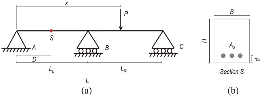
Given that $R_{\epsilon }^{\mathrm{I}}$ consists of structure responses with opposite signs. This study adopts a two-span reinforced concrete continuous beam as a demonstration model, as depicted in Figure 1. Figure 1(a) provides a sketch of the continuous beam, while Figure 1(b) details the dimensions of the mid-span section ( $S$ ). The mid-span of the left span is chosen as the primary observation section, as this region experiences the maximum bending moment and is thus most vulnerable to damage. Accordingly, $R_{\epsilon }^{\mathrm{I}}$ is characterized as the maximum and minimum strains experienced at the section $S$ during the transit of a concentrated load $P$ . The maximum strain corresponds to the peak sagging moment recorded at section $S$ , while the minimum strain corresponds to the peak hogging moment.

Figure 1.

(a) Dimensions of the continuous beam, with the left and right span lengths denoted by L_L and L_R, respectively, and a total length of L. x and D denote the location of load P and section S, respectively. (b) Dimensions of section $S$ , with width B, height H, and reinforced area $A_s$ . d represents the rebar cover thickness.

Validation of qualitative diagnosis

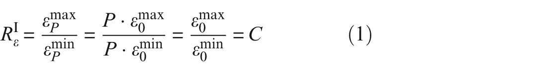
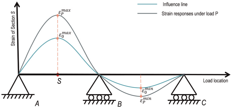
The two curves in Figure 2 depict the strain variations in the bottom fiber of section $S$ during the transition of a unit load and load $P$ , respectively. Although the response shapes are identical, their magnitudes differ, with the strain response under load P being proportional to that under unit load by a factor of P. Consequently, the damage feature extracted from both strain responses is expressed as

$$R_{\epsilon }^{\mathrm{I}}=\frac{{\epsilon }_P^{\max }}{{\epsilon }_P^{\min }}=\frac{P·{\epsilon }_0^{\max }}{P·{\epsilon }_0^{\min }}=\frac{{\epsilon }_0^{\max }}{{\epsilon }_0^{\min }}=C$$

(1)

where ${\epsilon }_{\mathrm{sP}}^{\max }$ and ${\epsilon }_{\mathrm{sP}}^{\min }$ denote the maximum and minimum strains on the response curve for the load $P$ , respectively. ${\epsilon }_0^{\max }$ and ${\epsilon }_0^{\min }$ denote the peak and valley strains on the response curve for the unit load, respectively.

Figure 2.

The strain responses of the bottom fiber of section $S$ under the transition of a unit load and load $P$ .

Equation (1) indicates that $R_{\epsilon }^{\mathrm{I}}$ at section $S$ remains constant regardless of the load magnitude but varies with changes in the shape of the SIL. The shape of the IL reflects the static properties of the structure, such as boundary conditions and section stiffness. In the healthy stage of the beam, the SIL shape remains unchanged, resulting in a constant value of $R_{\epsilon }^{\mathrm{I}}$ , denoted as $C$ , across different load magnitudes. However, in the damaged stage, the redistribution of loads alters the shape of the SIL, leading to variations in $R_{\epsilon }^{\mathrm{I}}$ . As the damaged structure transitions into a stable state, the SIL stabilizes into a new configuration distinct from the healthy stage. Consequently, $R_{\epsilon }^{\mathrm{I}}$ converges to a new constant value, $C^{\prime }$ , under different load magnitudes, analogous to its behavior in the healthy stage.

Derivation of quantitative diagnosis

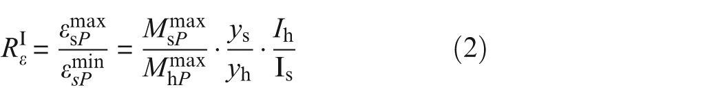
To further explore the relationship between the variations of $R_{\epsilon }^{\mathrm{I}}$ and the local health state of the structure, $R_{\epsilon }^{\mathrm{I}}$ is expressed using material mechanics, as

$$R_{\epsilon }^{\mathrm{I}}=\frac{{\epsilon }_{\mathrm{s}P}^{\max }}{{\epsilon }_{\mathrm{sP}}^{\min }}=\frac{M_{\mathrm{s}P}^{\max }}{M_{\mathrm{h}P}^{\max }}·\frac{y_{\mathrm{s}}}{y_{\mathrm{h}}}·\frac{I_{\mathrm{h}}}{{\mathrm{I}}_{\mathrm{s}}}$$

(2)

where $M_{\mathrm{s}P}^{\max }$ and $M_{\mathrm{h}P}^{\max }$ are the maximum sagging and hogging moments at section $S$ , respectively. $y_{\mathrm{s}}$ and $y_{\mathrm{h}}$ represent the distances from the NA to the bottom fiber when section $S$ is under sagging and hogging moments, respectively. Similarly, $I_{\mathrm{s}}$ and $I_{\mathrm{h}}$ are the corresponding second moments of area of section $S$ under sagging and hogging moments, respectively. Equation (2) indicates that $R_{\epsilon }^{\mathrm{I}}$ is influenced by the ratio of bending moments, the ratio of NA locations, and the ratio of the second moments of area.

Bridge damage often begins with minor defects, such as small cracks, which are difficult to detect using dynamic characteristics, such as natural frequency. This study focuses on the early stages of bridge damage, aiming to detect local structural defects before they propagate. It is assumed that local degradation occurs exclusively within section $S$ , and the resulting moment redistribution is confined to this section, leaving the moment IL of the beam unchanged. Accordingly, the ratio of the maximum sagging ( $M_{\mathrm{s}}^{\max }$ ) to hogging ( $M_{\mathrm{h}}^{\max }$ ) moments at section $S$ remain a constant value ( $C_{\mathrm{M}}$ ). Since the second moment of area I is directly influenced by the position of the NA, $R_{\epsilon }^{\mathrm{I}}$ is thus a function of the NA location. Consequently, shifts in $R_{\epsilon }^{\mathrm{I}}$ are closely correlated with shifts in the NA position.

NA shifts

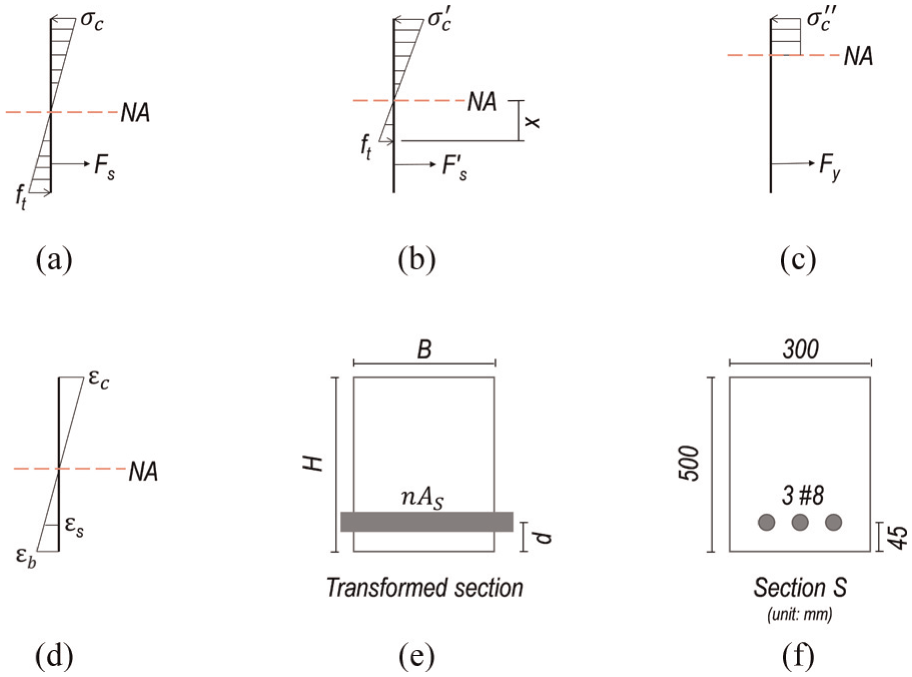
The location of the NA in a reinforced concrete section provides key insights into its design and material properties. Any changes in section design or degradation of materials can cause shifts in the NA location. In highway bridges, cracking is a primary factor contributing to these shifts, as it reduces the height of the concrete tension zone and alters the structural behavior of the section. This section discusses the shifts of the NA location ( ${\mathrm{y}}_{\mathrm{s}}$ ) and its corresponding shifts of the second moment of area ( $I_{\mathrm{s}}$ ) within section $S$ as cracking progresses under an increasing sagging moment. In this study, the NA location is defined as the distance between the NA and the bottom fiber of the section. Figure 3(a) to (c) illustrates the stress distribution in section $S$ under increasing sagging moments, depicting its evolution from an uncracked state to a partially cracked state, and ultimately to a fully cracked state, where the NA gradually shifts toward the top fiber. The strain distribution during the cracking process is assumed to remain unchanged, as shown in Figure 3(d).

Figure 3.

(a) NA position before section cracking. (b) NA position of partially cracked section. (c) NA position of fully cracked section. (d) Strain distribution within section S. (e) Transformed section of section S. (f) Sectional dimensions of section S.

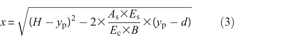
Before cracking, the entire concrete cross-section within section $S$ contributes to moment resistance, with the NA location ( $y_{\mathrm{b}}$ ) and second moment of area ( $I_{\mathrm{b}}$ ) determined using the transformed section illustrated in Figure 3(e). When the stress at the bottom fiber reaches the tensile strength ( $f_{\mathrm{t}}$ ) of the concrete, cracking initiates, causing the NA to shift due to the reduction in the effective tension zone, and the corresponding cracking moment is denoted by $M_{\mathrm{cr}}$ .

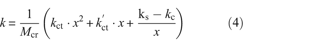
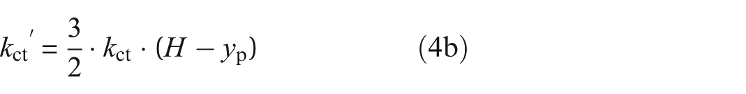
When the section enters into the partially cracked stage, the moment required to crack the bottom fiber of the tension zone is expressed as $k·M_{\mathrm{cr}}$ , where $k$ ranges from 1 to $\frac{M_{\mathrm{y}}}{M_{\mathrm{cr}}}$ , with $M_{\mathrm{y}}$ representing the yield moment of the reinforcing bars. When $k=M_{\mathrm{y}}/M_{\mathrm{cr}}$ , the section is considered fully cracked. By applying force and moment equilibrium conditions with the section dimensions in Figure 3(e), the relationships among parameter $k$ , the height of the tension zone ( $x$ ), and the NA location ( $y_{\mathrm{p}}$ ) can be derived as

$$x=\sqrt{{(H-y_{\mathrm{p}})}^2-2\times \frac{A_{\mathrm{s}}\times E_{\mathrm{s}}}{E_{\mathrm{c}}\times B}\times (y_{\mathrm{p}}-d)}$$

(3)

$$k=\frac{1}{M_{\mathrm{cr}}}(k_{\mathrm{ct}}·x^2+k_{\mathrm{ct}}^{\prime }·x+\frac{{\mathrm{k}}_{\mathrm{s}}-k_{\mathrm{c}}}{x})$$

(4)

$$k_{\mathrm{ct}}=\frac{1}{3}·E_{\mathrm{c}}·{\epsilon }_{\mathrm{t}}·B$$

(4a)

$${k_{\mathrm{ct}}}^{\prime }=\frac{3}{2}·k_{\mathrm{ct}}·(H-y_{\mathrm{p}})$$

(4b)

$$k_{\mathrm{s}}=A_{\mathrm{s}}·E_{\mathrm{s}}·{\epsilon }_{\mathrm{t}}·(H-d)·(y_{\mathrm{p}}-d)$$

(4c)

$$k_{\mathrm{c}}=\frac{1}{2}·k_{\mathrm{ct}}·(H-y_{\mathrm{p}}{)}^3$$

(4d)

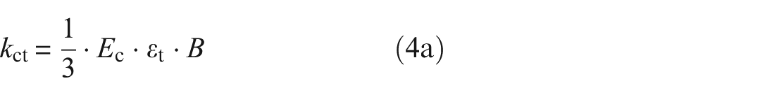
where $E_{\mathrm{c}}$ and $E_{\mathrm{s}}$ represent the Young’s modulus of concrete and rebars, respectively. ${\epsilon }_{\mathrm{t}}$ is the strain of the concrete when the stress reaches its tensile strength. $k_{\mathrm{ct}}$ , ${k_{\mathrm{ct}}}^{\prime }$ , $k_{\mathrm{s}}$ , and $k_{\mathrm{c}}$ , are coefficients of $x$ derived from the moment equilibrium within the section. The subscripts $\mathrm{ct}$ , $\mathrm{c}$ , and $\mathrm{s}$ indicate that the coefficients correspond to moments contributed by the concrete tension zone, compression zone, and rebars, respectively. The range of $k$ in this case is further extended to $[0,\frac{M_{\mathrm{y}}}{M_{\mathrm{cr}}}]$ to include the uncracked stage of the section, where $k\in [0,1]$ .

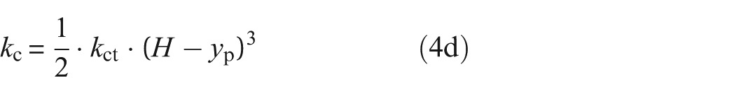
Using the sectional dimensions of section S shown in Figure 3(f) as an example, a detailed description of the NA shifts under increasing sagging moments is presented in Figure 4(a), while Figure 4(b) illustrates the corresponding changes in the second moment of area. For detailed calculation, the compression strength of concrete ( $f_{\mathrm{c}}^{\prime }$ ) is selected as $28\mathrm{MPa}$ , and thus its tensile strength ( $f_{\mathrm{t}}$ ) is calculated as $0.6·\sqrt{f_{\mathrm{c}}^{\prime }}$ . The Young’s modulus of concrete ( $E_{\mathrm{c}}$ ) is $25\mathrm{GPa}$ . Three No. 8 rebars are selected, with a Yong’s modulus ( $E_{\mathrm{s}}$ ) of $200\mathrm{GPa}$ and a yield strength ( $f_{\mathrm{y}}$ ) of $415\mathrm{MPa}$ .

Figure 4.

(a) NA shifts under sagging moment. (b) Second moment of area shifts correspond to the shifts of NA under sagging moment.

By computing the yield moment of the reinforcing bars, the range of parameter $k$ is determined as $[0,4.8]$ . During the uncracked stage of section $S$ , the NA location remains constant, resulting in a stable second moment of area. As cracking occurs, the section transitions into the partially cracked stage, where the NA shifts sharply away from the bottom fiber, causing a significant decrease in the second moment of area. Subsequently, the NA shifts gradually until reaching its final position in the fully cracked stage. In the example section shown in Figure 3(f), the NA location and the second moment of area stabilize at $344\mathrm{mm}$ and $1.47\times {10}^9{\mathrm{mm}}^4$ , respectively.

$R_{\epsilon }^{\mathrm{I}}$ shifts

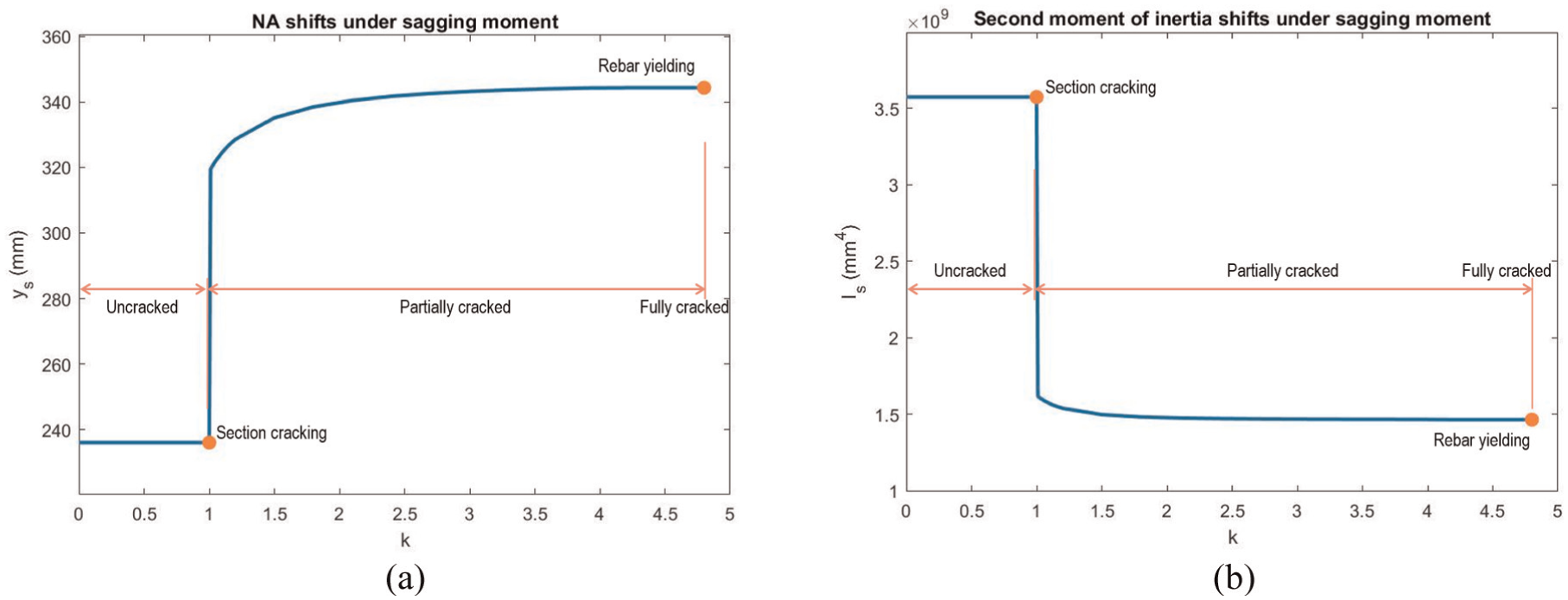
In mid-span sections, the hogging moment is relatively small compared to the sagging moment and rarely causes cracking at the top of the section. In addition, it is assumed that cracking in the concrete only affects its ability to carry tension, while under hogging moments, the cracked concrete below NA continues to contribute to resisting compression within the section. Therefore, when section $S$ is subjected to hogging moments under different health conditions, ranging from uncracked to partially cracked to fully cracked, its NA location and second moment of area remain constant as $y_{\mathrm{h}}$ and $I_{\mathrm{h}}$ , respectively. Therefore, the shifts of $R_{\epsilon }^{\mathrm{I}}$ is given by

$$\mathrm{Shift}(R_{\epsilon }^{\mathrm{I}})=C_{\mathrm{M}}·\mathrm{shift}\left(\frac{y_{\mathrm{s}}}{y_{\mathrm{h}}}\right)·\mathrm{shift}\left(\frac{I_{\mathrm{h}}}{I_{\mathrm{s}}}\right)$$

(5)

in which $y_{\mathrm{h}}$ and $I_{\mathrm{h}}$ equals to $y_{\mathrm{b}}$ and $I_{\mathrm{b}}$ , respectively.

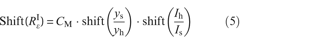
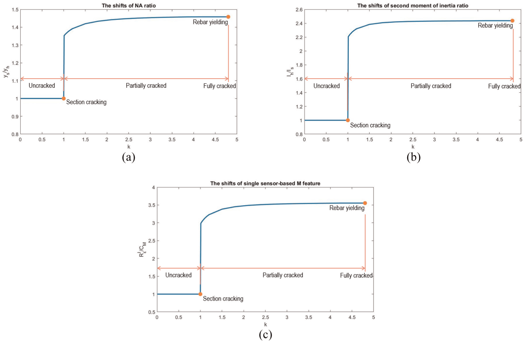
Employing the dimensions in Figure 3(f) as an example, the shifts in the NA ratio (y_s/y_h) under increasing sagging moments are illustrated in Figure 5(a), while Figure 5(b) shows the corresponding changes in the ratio of the second moments of area (I_h/I_s). Employing Equation (5), the shifts in $R_{\epsilon }^{\mathrm{I}}$ along the cracking stages of the section are presented in Figure 5(c), which demonstrates that the variations in $R_{\epsilon }^{\mathrm{I}}$ reflect the changes in the NA location under increasing sagging moments. Moreover, it is observed that the shifts in the NA caused by cracking are amplified when expressed in terms of $R_{\epsilon }^{\mathrm{I}}$ .

Figure 5.

(a) The shifts of NA ratio. (b) The shifts of second moment of area ratio. (c) The shifts of $R_{\epsilon }^{\mathrm{I}}$ .

Based on the relationship between the parameter $k$ and the cracking stages of the section, different values of $R_{\epsilon }^{\mathrm{I}}$ correspond to different cracking states. As shown in Figure 5(c), when $k\in [0,1]$ , $R_{\epsilon }^{\mathrm{I}}=C_{\mathrm{M}}$ , indicating an intact section. As $k$ approaches $4.8$ , $R_{\epsilon }^{\mathrm{I}}$ reaches $3.55C_{\mathrm{M}}$ , corresponding to a fully cracked section. Intermediate values of $k$ indicate a partially cracked section, during which $R_{\epsilon }^{\mathrm{I}}$ gradually deviates from $C_{\mathrm{M}}$ and approaches $3.55C_{\mathrm{M}}$ . The established relationship between $R_{\epsilon }^{\mathrm{I}}$ and the cracking stages enables the classification of the cracking state of a section using field measurements of $R_{\epsilon }^{\mathrm{I}}$ . In particular, if the precise section designs are available, the cracking depth can be determined by leveraging the correlation between $R_{\epsilon }^{\mathrm{I}}$ , the parameter $k$ , and the height of the concrete tension zone ( $x$ ).

Calculation of design value ( $C_{\mathrm{M}}$ )

As discussed in Section “Derivation of quantitative diagnosis,” when the structure is free from defects, the value of $R_{\epsilon }^{\mathrm{I}}$ remains constant at $C_{\mathrm{M}}$ . Assuming a uniform design of the bridge section, $C_{\mathrm{M}}$ is independent of the detailed section design and can serve as a benchmark for bridge condition assessment, particularly in cases where bridge design data is unavailable.

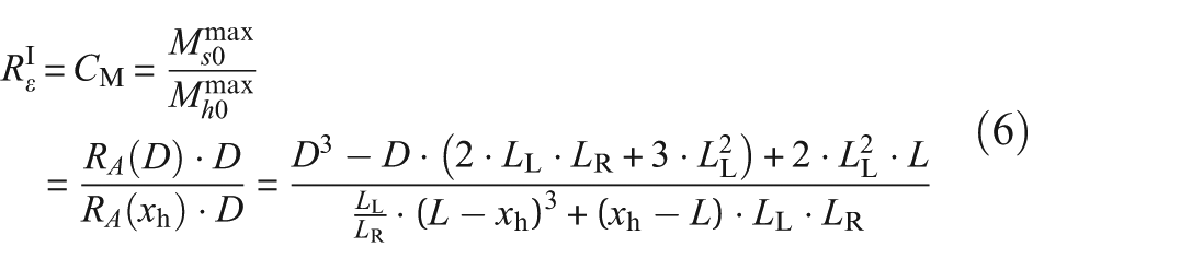
Take the left side of the section $S$ for observation in Figure 1, the bending moment, $M$ , at section $S$ , when the unit load travels from section $S$ to support $C$ , exhibits a linear relationship with the reaction at support $A,R(A)$ . By setting the first derivative of the mathematical model of $R(A)$ to zero, the load locations which cause the maximum and minimum bending moments at section $S$ are found to be at a distance of $D$ and $L-\frac{L_{\mathrm{R}}}{\sqrt{3}}$ away from the support $A$ , respectively. ²⁵

Accordingly, the design value for $R_{\epsilon }^{\mathrm{I}}$ is expressed as,

$$\begin{array}{c}{R}_{\epsilon }^{\mathrm{I}}=C_{\mathrm{M}}=\frac{M_{s0}^{\max }}{M_{h0}^{\max }}\hfill \\ =\frac{R_A\left(D\right)·D}{R_A\left(x_{\mathrm{h}}\right)·D}=\frac{D^3-D·(2·L_{\mathrm{L}}·L_{\mathrm{R}}+3·L_{\mathrm{L}}^2)+2·L_{\mathrm{L}}^2·L}{\frac{L_{\mathrm{L}}}{L_{\mathrm{R}}}·{(L-x_{\mathrm{h}})}^3+(x_{\mathrm{h}}-L)·L_{\mathrm{L}}·L_{\mathrm{R}}}\hfill \end{array}$$

(6)

The design value, $C_{\mathrm{M}}$ , of $R_{\epsilon }^{\mathrm{I}}$ , determined solely from the dimensions of the spans, represents the intact stage of the monitored structure, while the shifting of $R_{\epsilon }^{\mathrm{I}}$ from its design value indicates structural damage. For bridge local damage qualification, particularly in cases where design information is unavailable, the design value of $R_{\epsilon }^{\mathrm{I}}$ serves as a reliable benchmark, eliminating the need to collect baseline field data. As the example presented in Figure 5(c), the section condition can be categorized into uncracked, partially cracked, and fully cracked phases by comparing the field value of $R_{\epsilon }^{\mathrm{I}}$ with its design value.

Case study

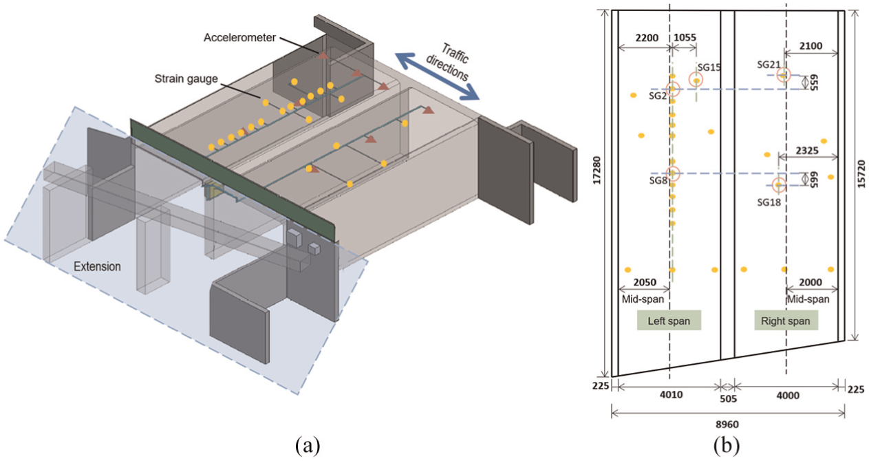
The Governor Macquarie Drive (GMD) Bridge, located in the suburb of New South Wales (NSW), Australia, is introduced as a case study to demonstrate the application of the design value of $R_{\epsilon }^{\mathrm{I}}$ in assessing bridge section health. This two-span reinforced concrete bridge was constructed approximately 30 years ago, and its original design information is unavailable. In February 2018, to accommodate increasing traffic demands, the GMD Bridge was extended, as illustrated in the 3D view provided in Figure 6(a).

Figure 6.

(a) 3D view of the GMD Bridge with the extension part highlighted. (b) Top view of the GMD Bridge with the layout of the SGs and the longitudinal dimensions.

To support bridge health management, a structural health monitoring (SHM) system comprising 27 strain gauges (SGs) and 18 accelerometers was installed to capture the vibrational responses of this bridge.^26–28 Since this study focuses on strain responses, the layout of the SGs is highlighted in the top view of the bridge with relevant dimensions measured, shown in Figure 6(b). The SGs were primarily installed under the mid-span and within the extension segment of the bridge.

Design value ( $C_{\mathrm{M}}$ ) calculation

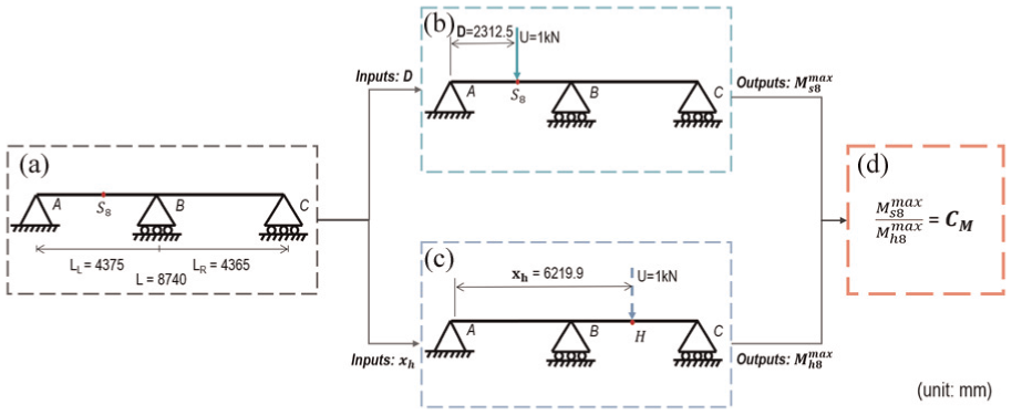
Since the entire deck of the GMD Bridge is firmly supported by three retaining walls, the structure can be simplified into several two-span continuous beams, as illustrated in Figure 7(a). The three retaining walls are modeled as supports positioned at the center of each wall. Under this simplification, the total span of the bridge is $8740\mathrm{mm}$ , with the left and right spans measuring $4375\mathrm{mm}$ and $4365\mathrm{mm}$ , respectively. For illustration purposes, this section focuses on the section at the location of SG8, denoted as $S_8$ .

Figure 7.

Flow chart of $C_{\mathrm{M}}$ calculation: (a) Simplified structure of the GMD Bridge, (b) structural system for maximum sagging moment calculation, (c) structural system for maximum hogging moment calculation, and (d) the application of Equation (6).

Assuming a uniform section design for the GMD Bridge, Figure 7 provides a flowchart detailing the calculation of $C_{\mathrm{M}}$ for $S_8$ , where the bridge is simplified as Figure 7(a). Figures 7(b) and 7(c) illustrate the structural systems used to compute the maximum sagging and hogging moments experienced at $S_8$ during the transition of a unit load, respectively. Assuming the unit load equals $1\mathrm{kN}$ , $R_A$ and $M_{S8}^{\max }$ are calculated as $0.3761\mathrm{kN}$ and $869.7271\mathrm{Nm}$ , respectively, with the distance between support $A$ and $S_8$ , $D$ , equals $2312.5\mathrm{mm}$ .

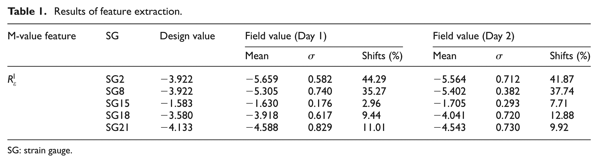
Similarly, the maximum hogging moment at $S_8$ during the transition of the unit load occurs when the unit load is at point $H$ . The distance between support $A$ and point $H$ ( $x_{\mathrm{h}}$ ) depends solely on the dimensions of the GMD Bridge, calculated as $6219.9\mathrm{mm}$ . The reaction in support $A$ is determined as $-0.0959\mathrm{kN}$ , and the maximum hogging moment, $M_{h8}^{\max }$ is computed as $-221.7578\mathrm{Nm}$ . Finally, applying Equation (6), as shown in Figure 7(d), the design value for $R_{\epsilon }^{\mathrm{I}}$ , that is, C_M, at $S_8$ is calculated to be $-3.9219$ . Since SG2 shares the same longitudinal location as SG8, both sensors yield the same design value. By substituting the specific locations of SG15, SG18, and SG21, along with the beam dimensions, into Equation (6), the corresponding design values are calculated and presented in Table 1.

Table 1.

Results of feature extraction.

M-value feature	SG	Design value	Field value (Day 1)			Field value (Day 2)
			Mean	σ	Shifts (%)	Mean	σ	Shifts (%)
$R_{\epsilon }^{\mathrm{I}}$	SG2	−3.922	−5.659	0.582	44.29	−5.564	0.712	41.87
	SG8	−3.922	−5.305	0.740	35.27	−5.402	0.382	37.74
	SG15	−1.583	−1.630	0.176	2.96	−1.705	0.293	7.71
	SG18	−3.580	−3.918	0.617	9.44	−4.041	0.720	12.88
	SG21	−4.133	−4.588	0.829	11.01	−4.543	0.730	9.92

SG: strain gauge.

Feature extraction

Signal preprocessing

Strain responses collected on two independent days, with an interval of half a month, were utilized to extract $R_{\epsilon }^{\mathrm{I}}$ . These measurements were taken during the operational stage of the bridge, recording longitudinal responses induced by random vehicles. These responses reflect the combined effects of vehicle-induced loading and existing structural conditions, and are not restricted to pure elastic or plastic behavior. However, the raw data contained noise induced by environmental disturbances, rendering it inappropriate for direct feature extraction. In addition, structural responses caused by individual axles of the vehicle during its transitions could not be isolated. To address these issues, this study employed the static strain responses of the structure for feature extraction, treating the passage of multi-axle vehicles as equivalent to a single concentrated load transition.

The sampling frequency of each SG was 200 Hz, and the on-site data was stored on a local server as .csv files, each containing one-minute periods of strain responses. To extract the static strain responses, the signals recorded in the .csv files were first decomposed using wavelet transforms and then reconstructed with the lower-frequency components. Daubechies wavelet transforms were chosen for this process due to their shape similarity with the signal.

Each strain dataset was decomposed to the default level in MATLAB, defined as

$$\mathrm{levels}=\mathrm{lo}{\mathrm{g}}_{2}N$$

(7)

where $N$ is the length of the signal. Given that each signal in the .csv files had a length of $12,000$ , the data was decomposed into $14$ levels. For signal reconstruction, the frequency threshold was set to $3\mathrm{Hz}$ , as suggested by the quality of the collected strain data. Based on the preprocessing of the data collected by all SGs, it is identified that the signals collected by SGs 2, 8, 15, 18 and 21 contained significant amplitudes induced by vehicles. The static strain responses from these gauges were further processed to isolate the components of the signals attributed to vehicle loads. The peaks and valleys of such signal components were then used to compute the field value of $R_{\epsilon }^{\mathrm{I}}$ .

Field value computation

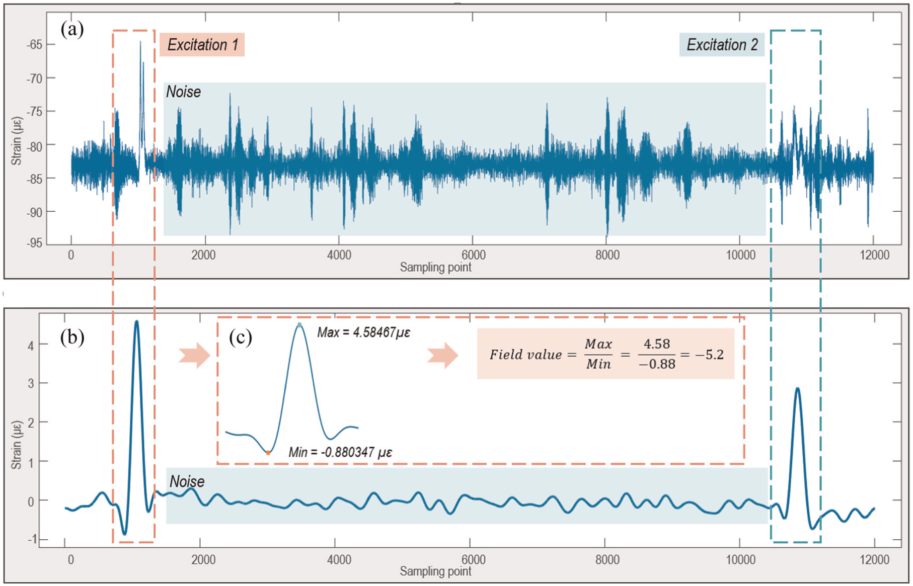
Figure 8 illustrates an example of the feature extraction process. Figure 8(a) shows a 1-min time history of strain data collected by SG8 on Day 1, while Figure 8(b) presents the corresponding static strain responses obtained after wavelet filtering. The value discrepancy between the two curves arises from the wavelet filtering applied during preprocessing, which removes the background noise, including instrument offset and the high-frequency bands, so as to only show the static component of the signal. Two periods of responses attributed to vehicle excitations are identified and highlighted in Figure 8, while other oscillations are classified as noise.

Figure 8.

Example of the feature extraction process: (a) One-minute raw data collected on Day 1, (b) the static responses extracted, and (c) peak and valley extraction.

Excitation 1 exhibits a significant amplitude that is clearly distinguishable from the noise in the raw data and has a well-defined peak and valley after static extraction. As shown in Figure 8(c), the maximum and minimum values of Excitation 1 are extracted, and their ratio is used to calculate the field value of $R_{\epsilon }^{\mathrm{I}}$ . In contrast, Excitation 2 has amplitudes similar to the noise. While a notable peak is observable after static extraction, its corresponding valley is obscured by noise. As a result, Excitation 2 is excluded from feature extraction.

By comparing these two excitations, Excitation 1 is interpreted as a single-vehicle traveling through the traffic lane containing SG8, whereas Excitation 2 is likely caused by a vehicle traveling on the adjacent lane of the bridge. To minimize the errors during the extraction of a single field value of $R_{\epsilon }^{\mathrm{I}}$ , $50$ signals similar to Excitation 1 are selected from the on-site collected data, resulting in $50$ corresponding field values. The mean of these $50$ field values is then calculated and used as the strain feature, representing the current condition of the section at SG8.

Results

To minimize errors caused by environmental disturbances and interference from vehicles traveling on adjacent lanes, only signals corresponding to single-vehicle crossings with significant and clear amplitudes were selected for feature extraction. These crossings were identified manually from the data collected during low-traffic periods, typically around midnight, when the passage of individual vehicles is more likely. Only two-axle vehicles were included to ensure that the resulting peaks and valleys corresponded to a uniform load. In the strain time histories, low-traffic volumes produced certain discrete signals. Only those with clearly defined single peaks and valleys were selected for analysis, as illustrated in Figure 8. Employing the extraction process detailed above, 10 datasets, each containing $50$ pairs of peaks and valleys, were extracted from the strain data collected by SG2, SG8, SG15, SG18, and SG21 on both Day 1 and Day 2.

Table 1 presents the mean and standard deviation of the extracted field values of $R_{\epsilon }^{\mathrm{I}}$ for the SGs, along with their design values. The shifts between the field values and the design values are also presented. All datasets yielded mean values with small standard deviations, indicating that the extracted strain features reliably reflect the current health state of the sections at the respective SG locations.

The single-sensor-based M-value feature is sensitive to damage that causes stiffness redistribution in the surrounding region, including cracks that are not directly beneath the gauge but still influence the local strain field. As previously mentioned, the GMD Bridge is an overpass located in a rural area of NSW, where cracking is the most common form of damage. These cracks may originate from various causes, including manufacturing defects, construction flaws, or deterioration over prior service periods. Once a crack is initiated, the NA of the cross-section shifts, which alters the internal strain distribution during subsequent bending. Consequently, even when the applied loads are below that for the cracking threshold and the measured strains remain within the elastic range, the strain profile differs from that of an undamaged section. The single-sensor-based M-value feature effectively captures this change, enabling the detection of damage under sub-cracking load conditions.

The results presented in Table 1 show that SG2 and SG8, located near the mid-span of the left span, exhibit the most significant shifts in $R_{\epsilon }^{\mathrm{I}}$ , indicating more severe damage in their surrounding regions. In contrast, SG15, positioned between the mid-span and the middle support of the same span, shows a smaller shift, with values below 8% on both days. These shifts are likely due to measurement variability or data noise rather than structural deterioration. SG18 and SG21, located around the mid-span of the right span, demonstrate similar $R_{\epsilon }^{\mathrm{I}}$ shifts of around 10%, suggesting the possible presence of minor cracking. These observations align with typical flexural damage patterns, in which the mid-span is more vulnerable to flexural cracks.

Comparing the results from the mid-span of the two spans, $R_{\epsilon }^{\mathrm{I}}$ values from SG2 and SG8 exhibit larger shifts than those from SG18 and SG21. One possible explanation is that SG2 and SG8 are situated closer to the primary vehicle wheel paths, thereby experiencing more intense and repeated loading over time. SG18 and SG21, on the other hand, are offset laterally by a similar distance from SG2 and SG8, respectively, resulting in reduced exposure to traffic loads and, consequently, exhibiting comparable and less severe damage. The spatial consistency between gauge locations and the observed gradients in the shifts of $R_{\epsilon }^{\mathrm{I}}$ reinforces the credibility of the results from both mechanical and structural perspectives, supporting the robustness of the proposed method.

Assuming that the shifts of $R_{\epsilon }^{\mathrm{I}}$ are caused by a single crack at the SG location, using the shifts in Section “Theoretical background” as a reference, where the shifts between $R_{\epsilon }^{\mathrm{I}}$ and $C_{\mathrm{M}}$ within the range of $(0,255\%)$ indicates a partially cracked section; the bridge sections at SG2 and SG8 are highly likely to be in the partially cracked stage. Comparing the shifts between SG2 and SG8, the section at SG2 with a higher field value may have a deeper crack depth than that at SG8. This difference may be attributed to local variations in material properties or traffic loading, even though both gauges are positioned at roughly the same longitudinal location. Considering that the GMD Bridge has been in service for decades, the presence of partially cracked sections in these areas is reasonable. Consequently, it can be inferred that the section at SG2 may have a lower load-bearing capacity than the section at SG8, achieving a similar conclusion in the literature that a higher M-value indicates lower load-bearing capacity. ²⁴ Furthermore, comparing the mean values of the same SG over two independent days suggests that the crack depth at both sections did not propagate during the half-month interval of data collection.

Discussion

Capabilities and limitations

The findings of this study conclude that $R_{\epsilon }^{\mathrm{I}}$ , derived from structural strain responses, serves as a reliable indicator for assessing bridge conditions both qualitatively and quantitatively. In terms of qualitative assessment, the variation of $R_{\epsilon }^{\mathrm{I}}$ indicates structural damage. It is able to detect damage caused by various factors, such as changes in boundary conditions and section cracking. Specifically, changes in boundary conditions result in alterations to the moment ratio, which are subsequently reflected in variations of $R_{\epsilon }^{\mathrm{I}}$ . Both minor and severe damage caused by section cracking are detectable using the feature, as such damage alters the shape of the ILs and shifts the position of the NA of local sections.

The calculation of the design value provides essential guidance for the qualitative assessment of bridge conditions, particularly in scenarios where sectional dimensions are unavailable or undocumented. As demonstrated in the case study, the strain feature extracted from on-site data was compared with its corresponding design value. By referencing the shifts presented in Section “Theoretical background,” the health condition of the bridge section can be categorized into uncracked, partially cracked, or fully cracked stages based on the scale of the shifts, thereby facilitating the prioritization and scheduling of on-site inspections and maintenance activities.

In contrast, the quantification of bridge damage is achieved by relating the crack depth to $R_{\epsilon }^{\mathrm{I}}$ . Detailed calculations of crack depth require design information, particularly the section properties of the structure. Furthermore, as moment redistribution among sections is not considered in the derivation process, the quantification capability of $R_{\epsilon }^{\mathrm{I}}$ is limited to minor damage, such as small cracks within sections. The single-sensor-based M-value feature, composed of strain components induced by both sagging and hogging moments, is inherently limited to diagnosing continuous and overhanging structures.

Compared with curvature-based strain features, the proposed $R_{\epsilon }^{\mathrm{I}}$ offers advantages in both design value derivation and field value extraction. To compute the design value, $R_{\epsilon }^{\mathrm{I}}$ requires only the span lengths and SG locations, making it particularly suitable for aging bridges where detailed structural drawings may be unavailable. In contrast, curvature-based methods typically rely on finite element analysis or the construction of theoretical ILs, adding complexity to the monitoring process. For field value extraction, $R_{\epsilon }^{\mathrm{I}}$ can be directly obtained from the peak tensile and compressive strains caused by ordinary traffic, without the need for controlled axle loads, traffic closures, or extensive calibration. By comparison, curvature-based approaches usually involve reconstructing the full SIL, which is more sensitive to noise and computationally intensive. The proposed $R_{\epsilon }^{\mathrm{I}}$ is therefore a more practical and robust option for damage detection in operational bridge environments.

Design value for multi-sensor-based M-value ( $R_{\epsilon }^{\mathrm{I}\mathrm{I}}$ )

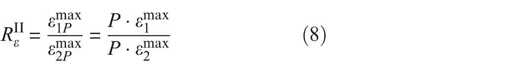
By extending the derivation of the design value of $R_{\epsilon }^{\mathrm{I}}$ , a theoretical basis can be further provided for $R_{\epsilon }^{\mathrm{I}\mathrm{I}}$ . By definition, $R_{\epsilon }^{\mathrm{I}\mathrm{I}}$ is expressed as

$$R_{\epsilon }^{\mathrm{I}\mathrm{I}}=\frac{{\epsilon }_{1P}^{\max }}{{\epsilon }_{2P}^{\max }}=\frac{P·{\epsilon }_1^{\max }}{P·{\epsilon }_2^{\max }}$$

(8)

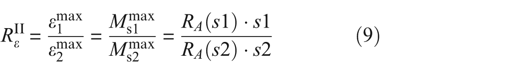
where ${\epsilon }_{1P}^{\max }$ and ${\epsilon }_{2P}^{\max }$ represent the maximum strains at sections 1 and 2, respectively, during the transition of load P. Similarly, ${\epsilon }_1^{\max }$ and ${\epsilon }_2^{\max }$ represent the maximum strains at sections 1 and 2, respectively, during the transition of a unit load. Assuming a constant $\mathrm{EI}$ between the sections, Equation (8) is expanded as

$$R_{\epsilon }^{\mathrm{I}\mathrm{I}}=\frac{{\epsilon }_1^{\max }}{{\epsilon }_2^{\max }}=\frac{M_{\mathrm{s}1}^{\max }}{M_{\mathrm{s}2}^{\max }}=\frac{R_A\left(s1\right)·s1}{R_A\left(s2\right)·s2}$$

(9)

where $M_{\mathrm{s}1}^{\max }$ and $M_{\mathrm{s}2}^{\max }$ denote the maximum sagging moments at sections 1 and 2, respectively, during the transition of a unit load. $s1$ represents the distance between section 1 and support A, while $s2$ denotes that between section 2 and support A. Equation (9) provides the design value for $R_{\epsilon }^{\mathrm{I}\mathrm{I}}$ , which depends solely on the structural dimensions and the locations of the sections.

Similar to the derivations for $R_{\epsilon }^{\mathrm{I}}$ , $R_{\epsilon }^{\mathrm{I}\mathrm{I}}$ can also be related to section designs and applied for stiffness comparisons between different sections. Unlike previous applications, such as that discussed in Yang and Ding, ²³ this approach can use any section for benchmarking rather than relying on a specific section that requires frequent maintenance.

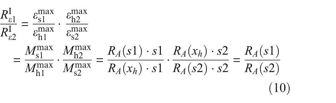
Taking the ratio of $R_{\epsilon }^{\mathrm{I}}$ at sections 1 and 2 yields

$$\begin{array}{c}\frac{R_{\epsilon 1}^{\mathrm{I}}}{R_{\epsilon 2}^{\mathrm{I}}}=\frac{{\epsilon }_{\mathrm{s}1}^{\max }}{{\epsilon }_{\mathrm{h}1}^{\max }}·\frac{{\epsilon }_{\mathrm{h}2}^{\max }}{{\epsilon }_{\mathrm{s}2}^{\max }}\hfill \\ =\frac{M_{\mathrm{s}1}^{\max }}{M_{\mathrm{h}1}^{\max }}·\frac{M_{\mathrm{h}2}^{\max }}{M_{\mathrm{s}2}^{\max }}=\frac{R_A\left(s1\right)·s1}{R_A\left(x_h\right)·s1}·\frac{R_A\left(x_h\right)·s2}{R_A\left(s2\right)·s2}=\frac{R_A\left(s1\right)}{R_A\left(s2\right)}\hfill \end{array}$$

(10)

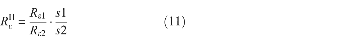
Equation (10) indicates that the ratio of $R_{\epsilon }^{\mathrm{I}}$ features in sections 1 and 2 corresponds to the ratio of the reactions at support A when the unit load is at sections 1 and 2, respectively. This relationship offers an alternative approach for timely bridge diagnosis. Employing Equations (9) and (10), $R_{\epsilon }^{\mathrm{I}\mathrm{I}}$ is related with $R_{\epsilon }^{\mathrm{I}}$ as

$$R_{\epsilon }^{\mathrm{I}\mathrm{I}}=\frac{R_{\epsilon 1}}{R_{\epsilon 2}}·\frac{s1}{s2}$$

(11)

When comparing the two types of features, $R_{\epsilon }^{\mathrm{I}\mathrm{I}}$ is not restricted by boundary conditions and can be applied to simply supported beams, whereas $R_{\epsilon }^{\mathrm{I}}$ is advantageous for structural assessment using only a single sensor. However, in the current configuration of the case study, where two SGs on the same transverse location with significant strain responses are unavailable, the verification of $R_{\epsilon }^{\mathrm{I}\mathrm{I}}$ cannot be achieved, but this study still provides the design value for $R_{\epsilon }^{\mathrm{I}\mathrm{I}}$ as a reference for future field or laboratory validations.

Conclusion

This study provided systematic theoretical support for the qualification and quantification of bridge damage detection using $R_{\epsilon }^{\mathrm{I}}$ feature, which is originally observed from field strain data. Its capability for qualifying bridge damage is validated and explained through the IL theories, while the quantitative diagnosis of minor bridge damage is achieved by establishing relationships between $R_{\epsilon }^{\mathrm{I}}$ and the depth of small cracks. In addition, the design value of $R_{\epsilon }^{\mathrm{I}}$ under the intact state of the structure is proposed, offering guidance for categorizing bridge damage and scheduling on-site inspections and maintenance activities. A case study involving a two-span reinforced concrete bridge demonstrates the application of $R_{\epsilon }^{\mathrm{I}}$ for bridge condition assessment in the absence of section design information.

The derivations in this study are limited to the detection of minor bridge defects using the M-value feature. Future research could explore the progression of the M-value shifts as minor sectional defects propagate into severe flexural failure. In practice, SGs are typically installed at structurally vulnerable locations, including the mid-span and regions near the supports, where cracks are more likely to occur due to the loading conditions. Future work should determine the sensitivity range of the M-value feature, defined as the greatest distance between a gauge and a crack and the smallest crack depth at that distance that can still be reliably detected, so as to optimize sensor layout and facilitate bridge monitoring. In addition, future studies could incorporate the effects of transverse loads in complex beam structures, such as girder bridges, by extending the IL to an influence surface to account for the multidimensional nature of the strain responses. Furthermore, the potential applications of the M-value feature for bridge prognosis, including its role in predicting future structural performance and informing maintenance planning, are worth investigation as well.