Sage Journals: Discover world-class research

Abstract

Bearing fault diagnosis is critical for the maintenance of mechanical systems. This paper proposes a transfer learning approach across different systems, faults, and signal types with limited labeled data. The core idea of this study is to integrate feature reshaping based on continuous wavelet transform and model fine-tuning, enhancing the model’s adaptability across different tasks. Feature reshaping based on spectral analysis improves the transferability of data within the model, while model fine-tuning aims to enhance diagnostic accuracy and accommodate the requirements of the target domain. To validate the feasibility and generalizability of the proposed method, two case studies were conducted. The results of case study 1 demonstrate that the method can achieve effective transfer learning across different machines, fault types, and label quantities, yielding high accuracy. Case study 2 explores transfer learning between different signal types, showing that acoustic signals can be successfully transferred to a vibration-based model. In addition, this paper uses Shapley Additive Explanation (SHAP) to interpret the transfer learning model. The SHAP analysis reveals that the model effectively captures the key time–frequency features associated with bearing faults. Feature reshaping enhances the signal-to-noise ratio, enabling the model to focus more on fault-related features rather than noise. SHAP analysis clearly highlights the feature differences between various fault types and identifies the critical factors underlying the model’s decision-making process. These findings validate the importance of feature reshaping and fine-tuning in improving the classification performance of the model.

Keywords

Convolution neutral network transfer learning bearing fault diagnosis bearing condition monitoring continuous wavelet transforms

Introduction

Bearings are essential components in rotating machinery and play a critical role in ensuring system stability and operational efficiency. Structurally, they consist of inner and outer rings, rolling elements, and cages. Due to continuous exposure to high loads and harsh operating environments, bearings are susceptible to degradation and eventual failure. Such failures can significantly reduce equipment performance or even cause unexpected shutdowns of entire systems, leading to substantial economic losses for industries.^1–3 As a result, early diagnosis and prognosis of bearing faults have become vital for enhancing equipment reliability and enabling predictive maintenance strategies.

To detect bearing faults at an early stage, various sensor signals—such as vibration, acoustic emission, and temperature—have been widely used.⁴ Among them, vibration signals are the most commonly applied due to their high sensitivity and ability to reflect dynamic changes in mechanical state.⁵ However, their effectiveness can be limited by signal attenuation, noise interference, or complex transmission paths in certain environments. In such cases, alternative signals such as acoustic emissions and temperature can offer complementary information. For instance, acoustic emission signals are effective in capturing early-stage crack formation, while temperature signals can reflect thermal variations caused by friction or insufficient lubrication. Therefore, it is important to develop diagnostic techniques that are adaptable across different systems and signal types.

Recently, deep learning techniques have been extensively investigated for bearing fault diagnosis and prognosis, owing to their strong ability to automatically learn complex patterns from large-scale data.^6–9 For example, Li et al.¹⁰ proposed a neural network-based method using time and frequency domain features of vibration signals for accurate fault detection under diverse working conditions. Similarly, He and He¹¹ adopted short-time Fourier transform (STFT) to preprocess acoustic emission signals and employed deep neural networks to enhance diagnostic performance. These methods demonstrate promising results when sufficient high-quality fault data are available. However, deep learning models heavily rely on the quantity and quality of training data.¹² In practical scenarios, fault samples are often limited due to the random and infrequent nature of mechanical failures, while normal condition data are relatively abundant. To address this issue, data augmentation techniques have been proposed to enrich training datasets.^13–17 Among them, virtual fault samples generated by simulating machinery operation and failure processes offer a low-risk solution, yet they may not fully capture the complexity and variability of real-world conditions. Consequently, the performance of deep learning models remains constrained by the scarcity of real fault data and challenges in replicating operational uncertainties.

Transfer learning has emerged as a solution to the data shortage by enabling a model trained on one task to transfer its knowledge to a related task.^18–21 For example, a model trained on data from similar machines can be adapted to a smaller dataset from a target machine, thereby leveraging existing data and reducing the need for extensive fault data.^22,23 Several researchers have investigated the transfer of bearing fault diagnosis models developed for one machine to other machines. For example, Kim et al.²⁴ proposed a domain adaptation method with semantic clustering for transfer learning between the same fault types across different machines. This statistic-based method can achieve about 90% accuracy, but it relies on thousands of target data samples to align feature distributions. Chen et al. proposed a transferable convolutional neural network (CNN) for bearing fault detection, which enables transfer learning between the same fault types across different machines.²⁵ This fine-tuning-based method enables cross-machine transfer learning but imposes strict requirements on fault types between target and source data and requires a large amount of data for training. Deng et al.²⁶ proposed a transfer learning method based on a double-layer attention-based adversarial network, which enables cross-system and cross-fault transfer learning. However, this method is limited in achieving high accuracy only when transferring between the same machine and fault modes. Its diagnostic accuracy decreases when applied to different systems and fault modes, and it also requires a relatively large amount of data. Overall, high accuracy in transfer learning has been typically achieved only when applied to the same or similar machines and faults. Transfer learning for bearing diagnosis using different signal types, such as acoustic, current, and vibration signals, remains unexplored.¹⁸ With the development of mechanical systems integrating multiple sensor technologies and considering the diversity of mechanical systems in real-world industrial applications, a transfer learning solution that can span different systems, fault types, and signal types is needed.

The “black box” nature of deep transfer learning models significantly limits their trustworthiness and reliability in high-risk applications, making interpretability analysis a key focus of research. Interpretability analysis aims to uncover the underlying logic and reasoning behind model predictions, enhancing model transparency and fostering user trust. Based on implementation strategies, interpretability methods can be categorized into two types: ante hoc and post hoc.²⁷ Typical post hoc techniques include class activation mapping (CAM),²⁸ Shapley Additive Explanations (SHAPs),²⁹ and Local Interpretable Model-Agnostic Explanations (LIME).³⁰ The advantage of these methods lies in their ability to retain the high performance of complex models while providing intuitive insights into the logic behind model decisions. For instance, CAM visualizes the regions of input features that are critical for model predictions, SHAP quantifies the contribution of each feature based on game theory, and LIME generates local linear approximations to explain individual predictions. These methods not only improve model transparency and user trust but also enhance the applicability of models in industrial settings.

This study proposes a novel transfer learning framework that enables cross-system, cross-fault-type, and cross-signal-type fault diagnosis using only a small amount of labeled data. By leveraging time–frequency representations generated via continuous wavelet transform (CWT), time-domain vibration and acoustic signals are converted into Red, Green, Blue (RGB) images that preserve both temporal and spectral information. A CNN is first pre-trained on a source domain dataset, and then adapted to diverse target domains through a spectral feature reshaping strategy and model fine-tuning, achieving high diagnostic accuracy under small-sample conditions.

In addition, this work introduces an interpretability analysis method that integrates CWT with SHAP. This method enables intuitive visualization of the model’s attention to key frequency regions and provides insight into the underlying causes of misclassifications. Compared to traditional diagnostic models, this approach not only improves generalization across heterogeneous domains but also enhances model transparency, supporting trustworthy deployment in real-world industrial applications.

The contribution of this is listed below:

This study proposes a transfer learning methodology that is simultaneously applicable to different bearing systems, fault types, and signal types under small-sample conditions.

A spectral feature reshaping strategy is introduced to enhance domain similarity, thereby improving transferability and enabling effective fine-tuning across heterogeneous systems and fault categories with limited data.

The proposed method is further validated on acoustic emission signals, demonstrating its generalizability across signal types and its potential to reduce data requirements, training time, and computational costs in real-world applications.

An interpretability framework combining CWT and SHAP is developed to visualize dominant frequency patterns and analyze the diagnostic errors.

The remainder of this paper is organized as follows: the second section provides an overview of the bearing systems and datasets used in this study, detailing their characteristics and diversity, and explaining the criteria for dataset selection. The third section describes the transfer learning methods employed, including CWT, CNN, feature reshaping, and the retraining and fine-tuning of the classification layer. The fourth section presents an experimental validation of the proposed method through case studies, evaluating its performance across different datasets by SHAP analysis. The fifth section discusses the Impact of training data scale on model performance, inter-class separability, and intra-class separability using SHAP analysis. The sixth section summarizes the main contributions of this study and discusses its limitations and directions for future work.

Dataset description

This paper uses different vibration datasets from different bearing systems and signal types to study transfer learning. These datasets include the Case Western Reserve University (CWRU) bearing dataset,³¹ the Intelligent Maintenance System (IMS) bearing dataset,³² the Machinery fault prevention technology (MFPT) bearing dataset,³³ Xi’an Jiaotong University-Sumyoung (XJTU-SY) bearing dataset,³⁴ Beijing Jiaotong University – Rail Autonomous Operations (BTJU-RAO) dataset,³⁵ and Korea Advanced Institute of Science and Technology (KAIST) bearing dataset.³⁶

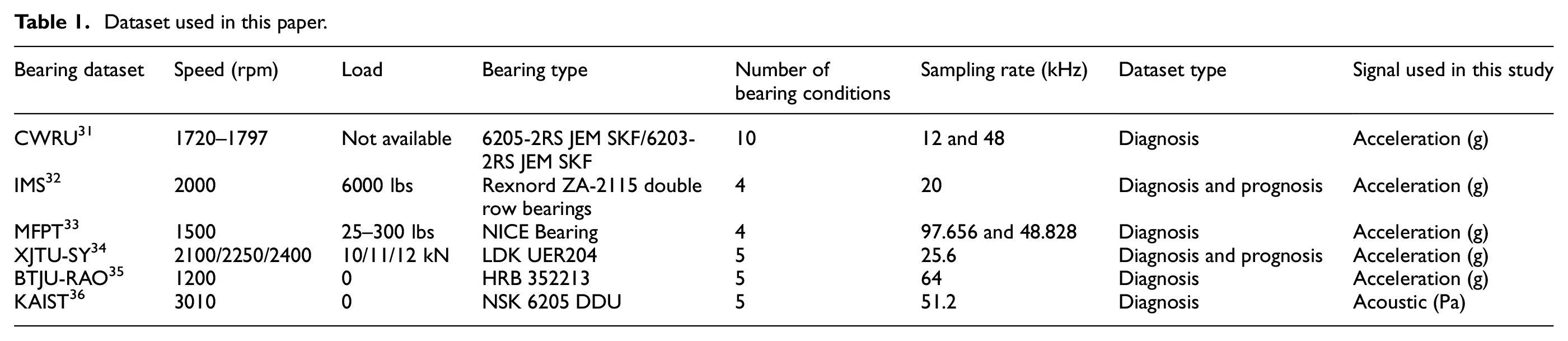
These datasets are collected from various bearing systems under different operating conditions, with detailed parameters provided in Table 1. The datasets vary in terms of rotational speed, load, bearing type, sensor type, sampling rate, signal-to-noise ratio (SNR), as well as the type and number of faults. In general, the theoretical bearing fault frequency can be calculated using the following equations³⁷:

Table 1.

Dataset used in this paper.

Bearing dataset	Speed (rpm)	Load	Bearing type	Number of bearing conditions	Sampling rate (kHz)	Dataset type	Signal used in this study
CWRU³¹	1720–1797	Not available	6205-2RS JEM SKF/6203-2RS JEM SKF	10	12 and 48	Diagnosis	Acceleration (g)
IMS³²	2000	6000 lbs	Rexnord ZA-2115 double row bearings	4	20	Diagnosis and prognosis	Acceleration (g)
MFPT³³	1500	25–300 lbs	NICE Bearing	4	97.656 and 48.828	Diagnosis	Acceleration (g)
XJTU-SY³⁴	2100/2250/2400	10/11/12 kN	LDK UER204	5	25.6	Diagnosis and prognosis	Acceleration (g)
BTJU-RAO³⁵	1200	0	HRB 352213	5	64	Diagnosis	Acceleration (g)
KAIST³⁶	3010	0	NSK 6205 DDU	5	51.2	Diagnosis	Acoustic (Pa)

Ball-pass frequency at outer race (BPFO):

\begin{matrix} BPFO = \frac{n f_{r}}{2} (1 - \frac{d}{D} \cos φ) \end{matrix}

(1)

Ball-pass frequency at inner race (BPFI):

\begin{matrix} BPFI = \frac{n f_{r}}{2} (1 + \frac{d}{D} \cos φ) \end{matrix}

(2)

Fundamental train frequency (FTF, cage speed):

\begin{matrix} FTF = \frac{f_{r}}{2} (1 - \frac{d}{D} \cos φ) \end{matrix}

(3)

Ball (roller) spin frequency (BSF):

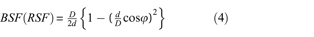
\begin{matrix} BSF (RSF) = \frac{D}{2 d} {1 - {(\frac{d}{D} \cos φ)}^{2}} \end{matrix}

(4)

where n is the number of rolling elements, d is the diameter of rolling element, D is the pitch diameter of the bearing, f_r is the speed of shaft, and φ indicates the angle of the load from the radial plane. From the above equations, it can be inferred that the structure of the bearing has a significant impact on the fault characteristic frequency. Additionally, the geometric dimension of the fault also affects the impact frequency of bearing faults.

These datasets include fault signals collected from various types of bearings under different fault severities and operating conditions. Among them, the CWRU bearing dataset provides the most comprehensive fault information, covering more than a dozen distinct fault types. Due to its diversity and richness, the CWRU dataset is used as the source domain for pre-training the model in this study. In addition, acceleration signals from the IMS, MFPT, and XJTU-SY datasets, as well as acoustic signals from the KAIST bearing dataset, are adopted as target datasets for transfer learning. The IMS and XJTU-SY datasets are collected during the later stages of bearing run-to-failure experiments, where the bearings exhibit severe damage and are subjected to high radial loads. MFPT and KAIST datasets are obtained from bearing rotation test rigs and represent relatively mild fault conditions. The BJTU-RAO dataset is collected from subway train bogies and is mainly used in this study for analyzing compound fault scenarios. To evaluate the effectiveness of the proposed method under small-sample conditions, only 300–400 samples from each target dataset are used for training. A relatively larger test set, typically containing several thousand samples, is used to assess the model’s accuracy and generalization performance.

Development of the proposed transfer learning method

The research methodology of this study is illustrated in Figure 1. First, time-domain vibration signals of 10 different bearing conditions are extracted from the CWRU dataset as the source dataset. This dataset includes various types and levels of bearing damage, which helps the neural network learn more detailed time–frequency domain signal characteristics. Subsequently, these time-domain signals are transformed into scalograms with both time and frequency information through CWT. The CWT process not only reveals the intrinsic dynamic characteristics of the signals but also captures the frequency variations over time in detail. The obtained time–frequency data are then converted into RGB images, making the nonlinear and non-stationary signal features visually intuitive. Each image is labeled according to the corresponding bearing condition, which is a crucial step for subsequent supervised learning models. Finally, we trained a CNN using these labeled image data. By fine-tuning the network structure and hyperparameters and conducting a series of tests, we could achieve a highly accurate pre-trained model that learned numerous bearing fault characteristics.

Figure 1.

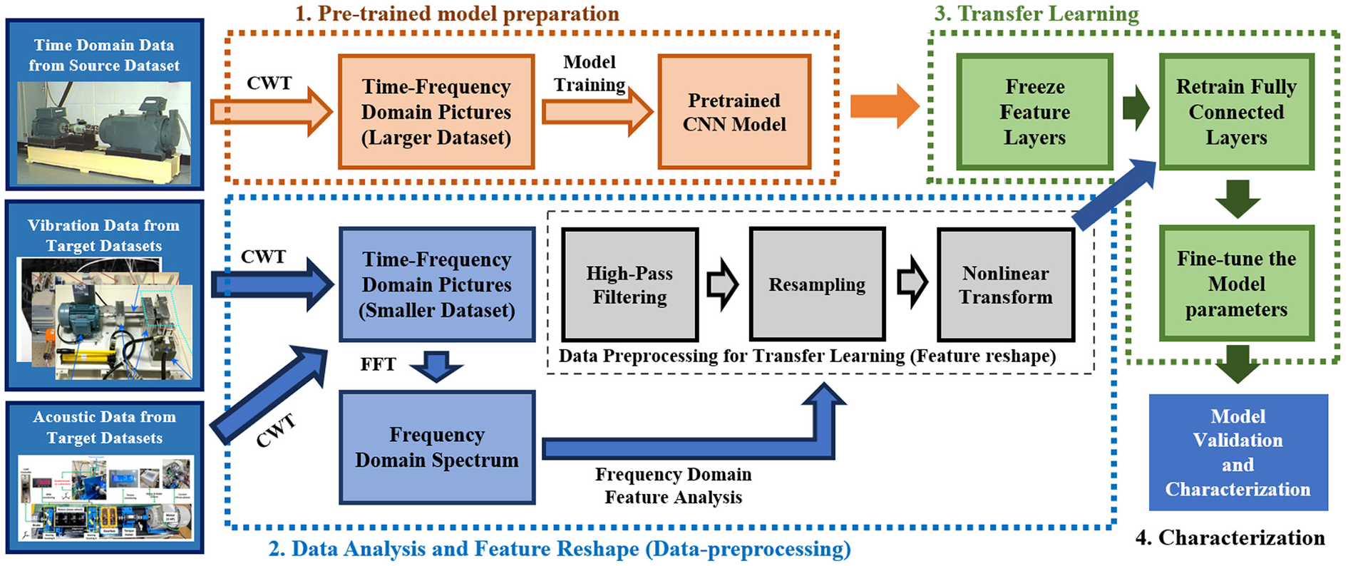
Schematic diagram of the proposed methodology.

Next, partial time-domain vibration signals and acoustic signals from other bearing datasets are selected as the target dataset to validate and characterize the proposed transfer learning method. Due to differences in bearing type, sampling rate, rotational speed, and load between different bearing systems, the frequency-domain and time-domain information of the signals are inconsistent, posing challenges for transfer learning. This study proposes a concise and novel data preprocessing method based on frequency domain analysis and RGB wavelet images to enhance the transferability of data on the source model. These preprocessing steps ensured that data from different sources had consistent formats and scales before being input into the pre-trained model. To gain deeper insights into the frequency-domain characteristics of the target dataset, fast Fourier transform (FFT) is used to analyze the spectrum. FFT enables the identification and analysis of frequency characteristics of the target data under different bearing conditions. By comparing the spectral characteristics of the target dataset with those of the source dataset, we assessed their similarities and differences. Based on these observations, the target signals underwent filtering, denoising, and feature reshaping during the CWT process to make the features of the target dataset resemble those of the source dataset. In this process, the features of the time-domain signals are normalized and visualized, which not only effectively removed noise from the data but also enhanced key features in the signals, making them more suitable for transfer learning.

Then, we adopt a strategy of freezing and fine-tuning parameters on the pre-trained CNN to achieve transfer learning between different mechanical systems, bearing fault and signal types. In different mechanical systems, varying types and severities of bearing damage can result in time–frequency domain pattern changes similar to those in the source dataset. Similarly, in acoustic data, different bearing faults produce corresponding time–frequency domain signal variations, even if these changes are very subtle. Specifically, all convolutional layers and some fully connected layers are frozen to retain the feature extraction capabilities learned from the source dataset while retraining the final fully connected layers to adjust and optimize model parameters to fit the new target dataset. Then, certain parameters in the model’s feature layers are fine-tuned during the training process to further improve model accuracy. Through this approach, the model could effectively adapt to the new data environment while retaining learned features, thereby enhancing diagnostic accuracy and generalization capability. This transfer learning method not only accelerated the model training process but also significantly improved the model’s performance on the new dataset.

Finally, to further validate the effectiveness of the proposed method, this study employs a combination of CWT and SHAP for interpretability analysis of the model. The SHAP analysis reveals that the pre-trained model successfully captured the key feature regions corresponding to different bearing conditions. After applying transfer learning, the SHAP value distributions on the target dataset clearly highlighted the model’s focus on time–frequency domain features, reflecting its basis for distinguishing various fault modes. Compared to models without fine-tuning or feature reshaping, the proposed method significantly improved the recognition of complex fault features while reducing the interference of noise on the model’s decision-making process, thereby further validating the effectiveness of feature reshaping and fine-tuning.

The innovation of this method lies in the integration of feature reshaping, model fine-tuning, and SHAP interpretable analysis, enabling transfer learning to be effectively applied across different systems, fault types, and signal types. The following sections will provide a detailed explanation of these methods.

Time–frequency methods

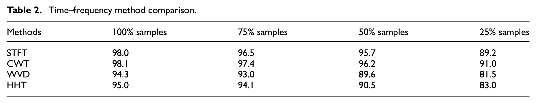
This study employs time–frequency methods to convert raw vibration signals into images. This study investigates four commonly used time–frequency methods: STFT, Wigner–Ville distribution (WVD), Hilbert–Huang transform (HHT), and CWT and compares their performance in fault classification tasks. The experiments are carried out using the source dataset and the VGG-16 model for image-based classification. The structure of VGG-16, its training settings, and the reasons for choosing it are described in detail in the next section. The study investigates how the accuracy of each time–frequency method changes with different amounts of training data, from 100 to 25% of the full dataset. In this case, 100% corresponds to a training set of 5460 samples. The results show that CWT has the highest classification accuracy, indicating its suitability for this task. The time–frequency method comparison is shown in Table 2.

Table 2.

Time–frequency method comparison.

Methods	100% samples	75% samples	50% samples	25% samples
STFT	98.0	96.5	95.7	89.2
CWT	98.1	97.4	96.2	91.0
WVD	94.3	93.0	89.6	81.5
HHT	95.0	94.1	90.5	83.0

The wavelet transform is a powerful mathematical tool for decomposing a signal into components at various scales and positions. It is particularly effective for analyzing signals with non-stationary or time-varying characteristics. Compared to the commonly used FFT, the wavelet transform offers significant advantages in accurately capturing both time and frequency information. This makes it ideal for revealing the intrinsic structure of one-dimensional data, especially across different scales, allowing for the extraction of valuable information tailored to specific application needs. The signal is decomposed using a series of fundamental functions called mother wavelets, which can be scaled and translated to match different features of the signal. The mathematical expression of CWT is³⁸

\begin{matrix} W_{f} (a, b) = \frac{1}{{| a |}^{\frac{1}{2}}} \int_{- \infty}^{+ \infty} x (t) \bar{ψ} (\frac{t - b}{a}) dt \end{matrix}

(5)

where x(t) represents the time-domain signal being analyzed, while ψ is the mother wavelet function and $\bar{ψ}$ represents the complex conjugate of the wavelet function. The parameter $a$ , a positive real number, controls the scale of the wavelet, and $b$ is the translation parameter, determining its shift along the time axis. W_f (a,b) denotes the wavelet transform of the signal x(t) at scale $a$ and translation $b$ . The inclusion of the complex conjugate $\bar{ψ}$ ensures the completeness and accuracy of the wavelet transform.

This study employs the complex Morlet wavelet as the mother wavelet, which integrates a sine wave modulated by a Gaussian envelope, offering a smooth representation in both the time and frequency domains. The complex Morlet wavelet is mathematically expressed as³⁸:

\begin{matrix} ψ (t) = ψ_{M} (t) = \frac{1}{\sqrt{π f_{b}}} e^{j 2 π f_{c} t} e^{- \frac{t^{2}}{f_{b}}} \end{matrix}

(6)

where $f_{c}$ denotes the center frequency and $f_{b}$ represents the variance or bandwidth. The complex Morlet wavelet is well-suited for capturing local signal features, such as edges and spikes, with high accuracy. Its adaptable frequency characteristic simplifies handling, while its continuous differentiability within the domain facilitates signal processing tasks. A time window of 400 sample points is selected, as excessively large or small windows could either compress or exaggerate features, making it difficult for CNNs to effectively recognize time–frequency domain characteristics. To balance resolution on the frequency axis, the scale parameter is set to 128. Figure 2 shows an example of a bearing vibration time-domain signal and its corresponding wavelet scalogram. Through Equations (5) and (6), the one-dimensional time-domain signal shown in Figure 2(a) can be converted into a two-dimensional signal, with the magnitude of the two-dimensional signal represented using a jet colormap, as shown in Figure 2(b). In the time-domain signal plot, the horizontal axis represents time, while the vertical axis represents signal amplitude, reflecting the dynamic changes of the signal over time. In contrast, the image produced by CWT illustrates the local characteristics of the signal in both time and frequency domains, where the horizontal axis still represents time, and the vertical axis represents frequency. Utilizing the jet colormap, different colors correspond to the signal strength at specific time and frequency points. The wavelet transform reveals the instantaneous variations in the time-domain signal, providing a more intuitive representation of its characteristics across different frequency ranges, thereby enhancing the effectiveness of subsequent feature extraction and pattern recognition. To meet the input requirements of CNNs, the time–frequency domain images are processed by removing their coordinate axes and resizing them to 224 × 224 × 3 RGB format.

Figure 2.

Transfer time-domain signal to time–frequency domain image by using CWT: (a) time domain and (b) time–frequency domain. CWT: continuous wavelet transform.

Convolution neural network and training

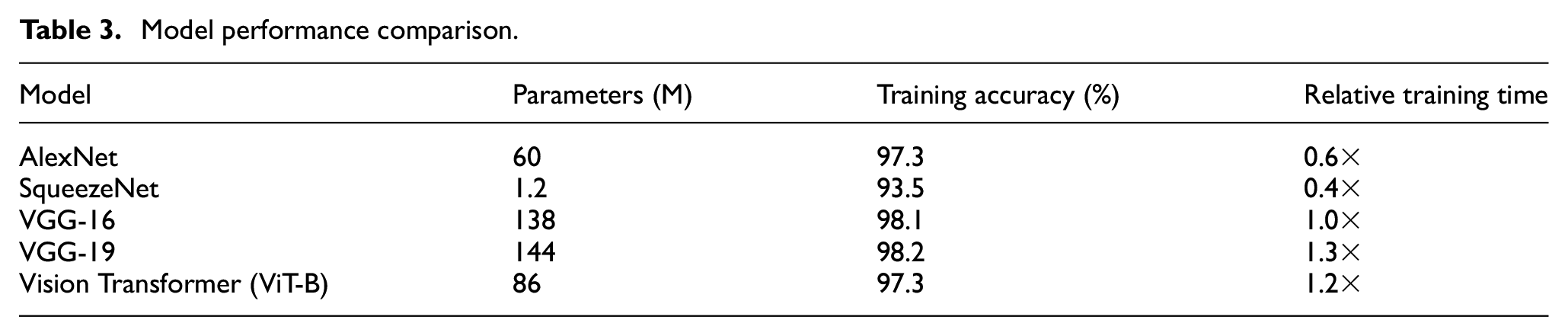
To identify a suitable baseline model for the proposed transfer learning framework, we perform comparative experiments using the complete source dataset. Several widely used architectures are evaluated, including AlexNet, SqueezeNet, VGG-16, VGG-19, and a Vision Transformer (ViT-B/16). As shown in Table 3, although AlexNet and SqueezeNet are computationally efficient, their classification accuracy is significantly lower, likely due to their limited feature extraction capabilities. VGG-19 achieves a similar level of accuracy to VGG-16 but requires longer training time and has a larger model size, offering no clear benefit. Although the Vision Transformer performs well on large-scale datasets, it does not provide a clear advantage on small- or medium-sized datasets. Based on these results, VGG-16 is selected as the baseline model due to its well-balanced performance in terms of accuracy, training efficiency, and model complexity. Its ability to extract stable and transferable features makes it particularly suitable for small-sample fault diagnosis tasks.

Table 3.

Model performance comparison.

Model	Parameters (M)	Training accuracy (%)	Relative training time
AlexNet	60	97.3	0.6×
SqueezeNet	1.2	93.5	0.4×
VGG-16	138	98.1	1.0×
VGG-19	144	98.2	1.3×
Vision Transformer (ViT-B)	86	97.3	1.2×

VGG-16 used in this study is illustrated in Figure 3.^39,40 It consists of 13 convolutional layers, 5 pooling layers, and 3 fully connected layers. The convolutional layers are primarily responsible for extracting relevant features from the input images, while the pooling layers, employing max pooling, reduce the spatial dimensions, that is, height and width, of the feature maps. This dimensionality reduction not only lowers computational costs but also helps mitigate overfitting. The fully connected layers transform the extracted feature maps into the final output, allowing VGG-16 to efficiently process and classify image data. The last six layers of the CNN model are further optimized through fine-tuning to adapt to specific target tasks, thereby enhancing the model’s performance on new datasets. t-Distributed stochastic neighbor embedding (t-SNE) analysis is used to visualize the distribution of the high-dimensional feature space in fully connected layer, revealing the relationships between different classes. Furthermore, with wavelet images as input, SHAP is employed for interpretability analysis, identifying the key regions involved in time–frequency feature extraction and classification decisions. This approach not only improves the model’s predictive accuracy but also deepens the understanding of its internal mechanisms.

Figure 3.

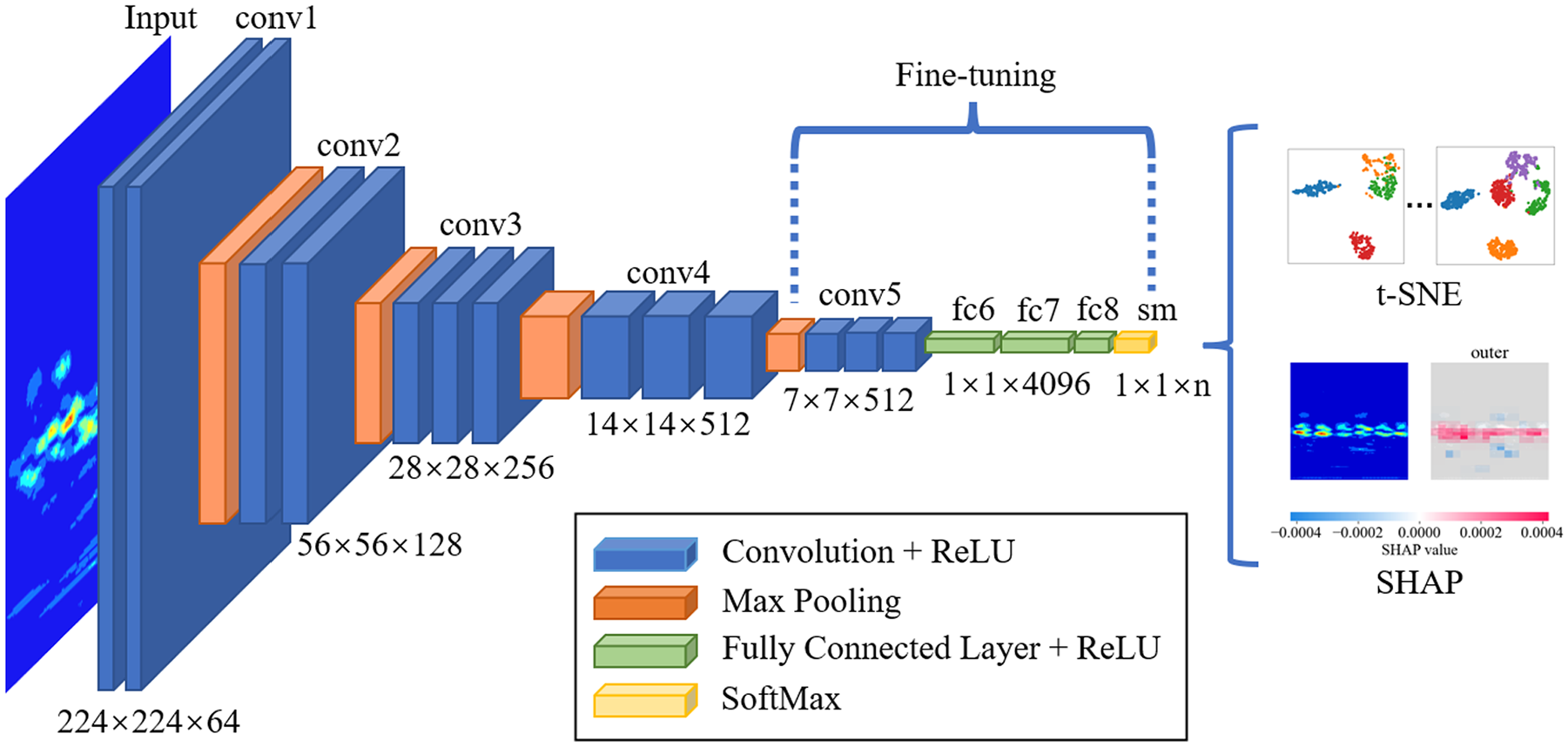
CNN architecture with t-SNE and SHAP. CNN: convolutional neural network; t-SNE: t-distributed stochastic neighbor embedding; SHAP: Shapley Additive Explanation.

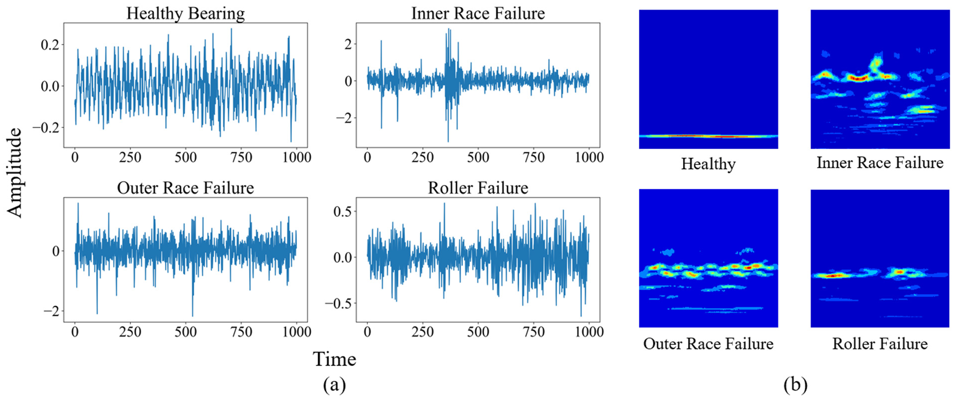
This study uses time–frequency images representing 10 different bearing conditions from the CWRU bearing dataset as input, with the corresponding bearing states serving as labels for model training. The training process utilizes the Adam optimizer with a batch size of 32 and a learning rate of 1e-5. The model is implemented in a Python 3.12.0 environment using the PyTorch 1.10.1 framework. The dataset is divided into a training set of 5460 samples, a validation set of 1560 samples, and a test set of 780 samples. The dataset comprises healthy bearings and bearings with outer race, inner race, and rolling element damages at depths of 7, 14, and 21 mil, resulting in a total of 10 labels.

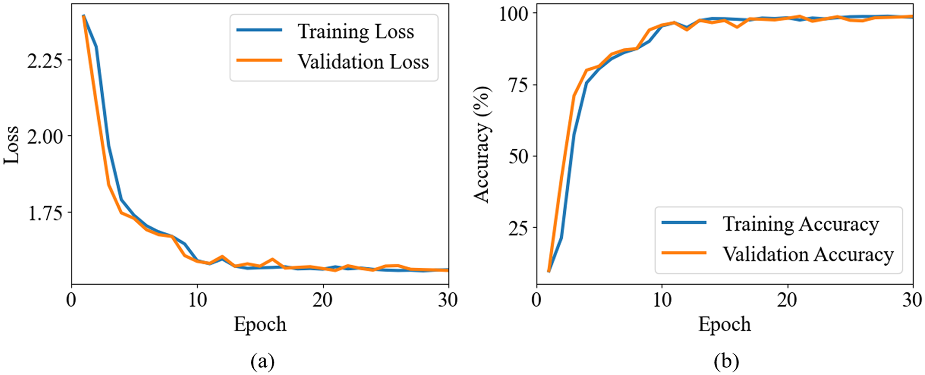
The training results of the VGG-16 model are presented in Figure 4. Figure 4(a) illustrates the reduction in loss values over the course of training, while Figure 4(b) depicts the gradual improvement in accuracy as the model is trained. This training process involved fine-tuning the model’s architecture and hyperparameters to optimize its performance. After extensive testing and validation, the model achieved an accuracy of up to 99.8% on the validation set.

Figure 4.

Training results of the pretrained CNN model: (a) training loss and (b) training accuracy. CNN: convolutional neural network.

We then evaluated the trained model using an independent test set to verify its performance. During this evaluation, a confusion matrix is generated, as shown in Figure 5, providing a detailed view of the model’s classification accuracy across different categories. Confusion matrix typically contains four key elements: true positive (TP), true negative (TN), false positive (FP), and false negative (FN). Accuracy is defined as the proportion of correctly predicted samples to the total number of samples, and the specific calculation formula is as follows:

\begin{matrix} Accuracy = \frac{TP + TN}{TP + TN + FP + FN} \end{matrix}

(7)

Figure 5.

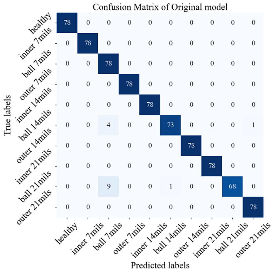
Confusion matrix of the model generated from the CWRU bearing dataset. CWRU: Case Western Reserve University.

TP and TN represent the number of samples that the model correctly predicts as positive and negative, respectively, while FP and FN represent the number of samples that the model incorrectly predicts as positive and negative, respectively. This formula can be used to evaluate the overall performance of the classification model. The results reveal that the model achieved an overall accuracy of 98.1%, indicating a high level of classification precision and reliability. The misclassification of certain images can be attributed to similarities in feature patterns among different classes, which may lead to ambiguity in the model’s decision-making process. This strong performance demonstrates the model’s robustness in accurately identifying and distinguishing between different bearing conditions.

Proposed framework for transfer learning

Transfer learning generally relies on the assumption that different types of features in different systems or situations share some common rules that are difficult to describe but can be represented through machine learning or deep learning. Commonly used transfer learning methods include statistical-based methods, adversarial-based methods, and fine-tune-based methods, each with its own strengths and limitations.¹⁸ Statistical methods achieve cross-domain feature alignment by measuring the distributional differences between source and target domains, requiring no target domain labels and offering ease of deployment. However, these methods are less effective in handling complex problems with label inconsistencies, tend to yield moderate accuracy, and have high data requirements. Adversarial methods leverage generative adversarial networks by incorporating discriminator modules to generate domain-invariant features, making them suitable for handling multiple working conditions and diverse machine faults. Nevertheless, they involve challenging optimization, high dependence on target data volume and computational resources, and are difficult to apply in practice. Fine-tuning, on the other hand, relies on target domain labels to adjust model parameters, achieving high diagnostic accuracy even with inconsistent label sets. However, when significant distributional differences exist between the source and target domains, and the training dataset is relatively small, the model is prone to becoming trapped in a local optimum, leading to a notable decline in testing accuracy. To address this challenge, this paper proposes a data preprocessing and feature reshaping strategy tailored for fine-tuning in transfer learning. This approach effectively overcomes accuracy degradation caused by local optima in small-sample scenarios. By enhancing the similarity between source and target domain data, it significantly mitigates performance degradation resulting from distributional discrepancies.

The transfer learning strategy adopted in this study is illustrated in Figure 6. A CNN model is first trained on the source dataset to obtain a pretrained model, which captures general low- and mid-level features such as edges, textures, and shape patterns in the time–frequency domain. These features typically exhibit strong generalization and are transferable across tasks. To enhance domain similarity, the target data is reshaped through spectral analysis to highlight its dominant frequency components and suppress noise. This preprocessing step improves the relevance of the target features to the source domain, thereby facilitating more effective transfer learning. Next, the pretrained model is adapted to the target task by freezing the early convolutional layers and retraining the fully connected layers. This allows the model to learn task-specific classification mappings while preserving transferable low-level representations. Finally, selected later convolutional layers and all fully connected layers are fine-tuned using the target data, further improving the model’s ability to extract and represent target-specific features. This approach integrates frequency-domain feature reshaping with adaptive fine-tuning, enabling effective knowledge transfer across different bearing systems and signal types. The following sections provide detailed validation through case studies.

Figure 6.

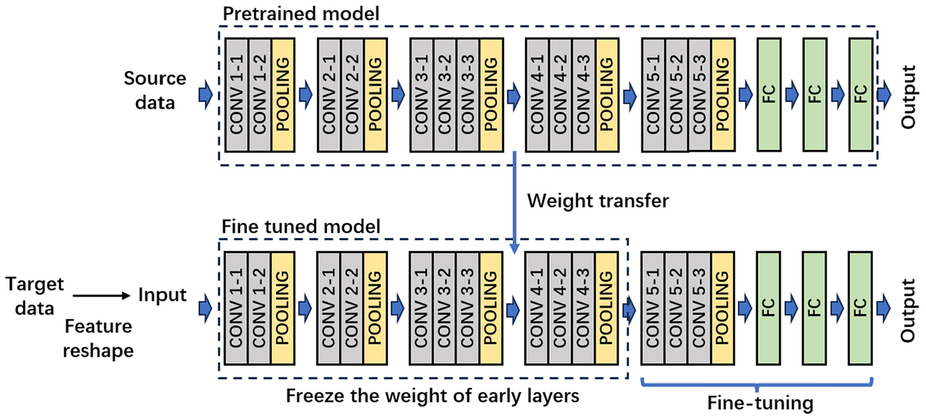
Basic framework of the proposed transfer learning.

Data preprocessing

The purpose of data preprocessing is to improve the transferability of the target datasets, especially since there are notable differences in system structure, bearing type, rotation speed, fault severity and type, and the number of categories among the datasets used in this study. These differences are described in detail in “Dataset description” section. In addition, although the SNR likely differs between datasets, explicit SNR values are not provided in the original sources and therefore are not included in the dataset description. To reduce the domain gap, preprocessing steps such as filtering and feature reshaping are applied. These steps help make the target data more consistent with the source data, enabling the CNN model to more effectively recognize fault patterns across different tasks.

Firstly, the frequency characteristics of the signal are obtained using FFT. Figure 7 shows examples of spectra for healthy and damaged bearing states from the source dataset, where all time-domain data are used to generate the spectrum. All continuous signals in the training set are used to generate the FFT, resulting in a complete spectrum. It can be observed that when the bearings are healthy, the main frequency components are located at low frequencies, with only one major peak. When the bearings are damaged, their main frequency components shift to higher frequencies, and multiple main frequency components appear. This is caused by the additional vibrations and impacts generated due to defects in the bearings. These impacts are very brief, containing higher frequency components, and thus appear as high-frequency peaks in the spectral analysis.

Figure 7.

Example of frequency spectrum analysis of the pretraining dataset: (a) FFT of healthy bearing and (b) FFT of damaged bearing. FFT: fast Fourier transform.

Figure 8 shows an example of the FFT for a segment of the signal from XJTU-SY dataset FFT results. From the figure, it can be observed that the spectrum of the healthy bearing is similar to that of the source dataset. However, the spectrum of the damaged bearing shows significant differences, with impact frequencies mainly appearing in the lower frequency range of the spectrum. This variation is due to differences in the bearing structure, working conditions, and sampling rate. If this signal is directly input into the model, it would not effectively identify potential fault patterns, making feature reshaping necessary.

Figure 8.

Example of frequency spectrum analysis of the XJTU-SY bearing dataset: (a) FFT of healthy bearing and (b) FFT of damaged bearing. FFT: fast Fourier transform.

Based on the spectral analysis results, feature reshaping can be applied to the signal. Initially, the DC offset and low-frequency noise must be removed, as shown in Figure 9. The presence of unremoved low-frequency components tends to dominate the time–frequency domain, obscuring the critical features of the signal and making them difficult to discern in time–frequency representations. Therefore, the removal of these interferences is a crucial step to ensure that the key signal characteristics are effectively highlighted during the analysis process. A third-order Butterworth high-pass filter with a cutoff frequency of 30 Hz is selected due to its smooth frequency response, absence of passband ripples, and low phase shift at high frequencies. As shown in the example in Figure 9, after removing low-frequency noise, the bearing fault features in the high-frequency range become more prominent and distinct, significantly enhancing the signal’s interpretability and the effectiveness of subsequent feature extraction.

Figure 9.

Example of high-pass filtering: (a) RGB wavelet picture before high-pass filtering and (b) RGB wavelet picture after high-pass filtering.

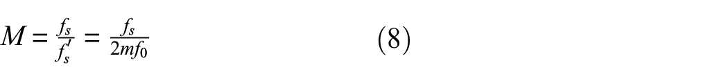
Due to variations in bearing types, operating conditions, sensor types, and data sampling rates across different datasets, impact frequencies may appear in the lower frequency range in some spectra, while in others, they may be located near the center of the frequency axis. In such cases, down sampling is required to shift the characteristic frequencies to the center of the spectrum. The down sampling factor M is determined by the following equation:

\begin{matrix} M = \frac{f_{s}}{f_{s}^{'}} = \frac{f_{s}}{2 m f_{0}} \end{matrix}

(8)

where $f_{s}$ is the sampling frequency, $f_{s}^{'}$ is the target sampling rate, and $f_{0}$ is the center frequency of the characteristic signal. $m$ is the bandwidth factor, which is set to 2 when shifting the characteristic frequency to the center of the spectrum.

In addition to the primary characteristic frequencies, the spectrum often contains other frequency components that differ from the main peaks. If the amplitudes of these frequency components are similar to those of the primary peaks, they can significantly interfere with the wavelet representation when converted into time–frequency images, resulting in mixed and unclear images that are difficult for CNNs to recognize. To address this, a nonlinear transformation method is employed to emphasize the frequency components with higher energy in the time–frequency images while diminishing the impact of secondary features, thereby enhancing the clarity of the time–frequency characteristics. The mathematical expression is

\begin{matrix} A = {A_{0}}^{k} \end{matrix}

(9)

where $A_{0}$ is the original amplitude from the wavelet transform, k is the parameter for the nonlinear transformation, and A is the wavelet amplitude obtained after the nonlinear transformation. With this approach, the proportion of the primary frequency component will increase relative to other components. When transformed into a jet colormap, the primary frequency component with higher amplitude will be prominently highlighted, displaying distinct features, while secondary frequency components and noise will blend into the blue background of the time–frequency image. This method enhances the primary features of the original signal, making them more easily recognizable by a pre-trained CNN without losing essential characteristics. An example of the nonlinear transformation is shown in Figure 10, where the left side displays the time–frequency image before non-linear transform, and the right side shows the denoised image obtained after the nonlinear transformation. The main frequency features are significantly enhanced, which is beneficial for CNNs to recognize fault patterns. In this application, k is chosen to be 2.

Figure 10.

Example of non-linear transform: (a) RGB wavelet picture before non-linear transform and (b) RGB wavelet picture after non-linear transform.

The purpose of data preprocessing is to enhance the transferability of the dataset, which is a critical step in transfer learning. Through processes such as filtering, feature reshaping, and nonlinear amplitude transformations, the signal characteristics of the target dataset become clearer and more closely aligned with those of the source dataset, thereby improving CNN-based recognition performance. This structured approach not only clarifies the features in time–frequency representations but also enables CNNs to accurately identify fault patterns across diverse datasets. The next chapter presents studies to verify and analyze the feasibility of the proposed method.

Shapley additive explanations

Compared to classic diagnosis models, interpretability in transfer learning places greater emphasis on global attribution consistency, which is essential for evaluating the effectiveness of transfer learning. In this study, SHAP was selected as the interpretability tool due to its ability to assign contribution scores to input features and support both local and global explanations. This allows for comparisons of feature attention patterns across different samples and domains, helping to reveal systematic shifts in model behavior before and after transfer. In contrast, commonly used methods such as CAM and LIME are limited in this context. CAM mainly provides coarse spatial maps tailored to CNNs, while LIME relies on local surrogate models sensitive to sampling, often resulting in unstable outputs under small-sample or cross-domain conditions. Moreover, both lack a framework for consistent global analysis. Therefore, SHAP provides a more robust and comprehensive approach to interpreting feature evolution and evaluating the effectiveness of transfer learning strategies.

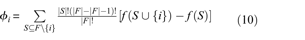
SHAP is a game-theory-based model explanation method designed to provide transparent interpretations of predictions made by complex machine learning models. Its core concept is derived from Shapley values, which allocate the contribution of each feature to the model’s output fairly, thereby helping to gain a deeper understanding of the model’s decision-making process. This method can provide both local explanations for individual samples and global insights into the model’s feature dependencies by aggregating results across multiple samples. For a sample $x$ , assuming its feature set is $F = {f_{1}, f_{2}, \dots, f_{n}}$ and the model’s prediction is $f (x)$ , the formula for Shapley values is⁴¹

\begin{matrix} ϕ_{i} = \sum_{S \subseteq F \ {i}} \frac{| S |! (| F | - | F | - 1)!}{| F |!} [f (S \cup {i}) - f (S)] \end{matrix}

(10)

where $S$ represents a subset of features excluding feature $i$ , and $| S |$ denotes the size of this subset, $f (S)$ is the model’s prediction based solely on the feature subset S, while $f (S \cup {i}) - f (S)$ quantifies the marginal contribution of feature $i$ to the model’s output.

In this study, CWT images are used as input features for the model to represent the time–frequency characteristics of the data. For each wavelet image sample $x$ , each pixel can be regarded as a feature. The SHAP method is utilized to quantify the contribution of each pixel or region to the classification outcome. Assuming the fault diagnosis model is represented as a function f, where x denotes the pixel matrix of the image and $f (x)$ is the predicted probability of classification, SHAP evaluates the contribution of a specific pixel i to the model’s prediction. To achieve this, SHAP constructs feature subsets $S$ , which are generated by masking or replacing certain pixels in the image. For each subset S, the model output $f (S)$ represents the predicted probability after removing specific pixels. Using the Shapley value formula, the SHAP method compares $f (S)$ and $f (S \cup {i})$ to quantify the marginal contribution of pixel $i$ . In CWT images, SHAP effectively highlights which time–frequency regions are most critical to the fault classification outcome, providing valuable insights for model interpretation and optimization. For instance, SHAP values can identify the most influential regions in wavelet images for classification outcomes, such as high- or low-frequency components during specific time intervals, thus revealing the model’s decision-making logic. Moreover, analyzing the distribution of SHAP values across multiple samples helps pinpoint the key features that models rely on for distinguishing fault categories. This not only improves interpretability but also optimizes feature selection, reducing unnecessary computational costs.

The magnitude and sign of the Shapley value directly indicate the contribution of a specific feature to the model’s prediction. The magnitude and sign of the Shapley value directly indicate the contribution of a specific feature to the model’s prediction. When the Shapley value is greater than 0, it indicates that the feature has a positive contribution, pushing the model’s prediction closer to the target value. When the Shapley value equals 0, it signifies that the feature has no influence on the prediction, meaning the model’s output remains unchanged regardless of whether the feature is included. When the Shapley value is <0, it shows that the feature has a negative contribution, driving the model’s prediction further away from the target. This interpretability is applicable for global evaluations by aggregating Shapley values across multiple samples. Such analyses provide valuable insights into feature importance, aiding in feature selection and model optimization.

More importantly, the SHAP method allows for an in-depth analysis of the causes behind classification errors, providing clear directions for model improvement. For instance, when a model relies on noise or secondary features for incorrect classifications, SHAP values can explicitly highlight the abnormal contribution of these irrelevant features to the classification outcome. This abnormal contribution may manifest as certain pixels or regions exhibiting disproportionately high SHAP values in incorrect classifications, even though these regions do not represent key features in correct classifications. Such scenarios often indicate overfitting, where the model excessively relies on noise patterns or background information in the data rather than learning discriminative features essential for accurate classification. By analyzing SHAP values, these erroneously amplified secondary features can be identified, enabling the introduction of denoising techniques during data preprocessing or the application of regularization constraints during training to reduce dependency on secondary features. Furthermore, such analyses may reveal limitations in specific feature extraction methods, such as the failure to eliminate redundant information in the data, leading to the model’s reliance on non-critical features. The insights provided by SHAP offer valuable guidance for optimizing feature extraction and data processing strategies.

Validation through case studies

Case study 1: transfer learning between different machines and faults

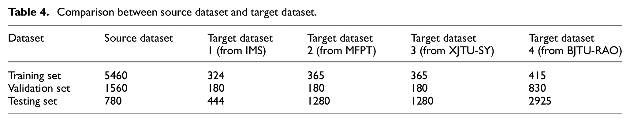
For training the transfer model, we use data from different bearing datasets, dividing them into smaller training and validation sets, each containing several hundred samples, along with a relatively larger test set. The aim is to more accurately evaluate the model’s generalization capability and validate the effectiveness and feasibility of the proposed method under small datasets. The basic information for each dataset is provided in Table 4. These datasets differ in terms of bearing damage conditions, types, operating conditions, and load characteristics. Target dataset 1, sourced from the IMS dataset, includes four bearing conditions: healthy bearings, inner ring damage, outer ring damage, and rolling element damage. The rotational speed is 2000 rpm, with a sampling rate of 20 kHz, and each damage condition operates under a radial load of 6000 lbs. The bearings used are double-row ball bearings. Target dataset 2, derived from the MFPT dataset, contains five conditions: healthy bearings, outer ring damage and inner ring damage with a radial load of 25 lbs, and outer ring damage and inner ring damage with a radial load of 300 lbs. The rotational speed is 1500 rpm, with sampling rates of 97.656 and 48.828 kHz, utilizing deep groove ball bearings. Target dataset 3, obtained from the XJTU-SY dataset, comprises four conditions: outer ring damage, mixed damage of the inner and outer rings, and cage damage. The rotational speed is 2400 rpm, the bearing type is a spherical bearing, the sampling rate is 51.2 kHz, and it operates under a radial load of 12 kN.

Table 4.

Comparison between source dataset and target dataset.

Dataset	Source dataset	Target dataset 1 (from IMS)	Target dataset 2 (from MFPT)	Target dataset 3 (from XJTU-SY)	Target dataset 4 (from BJTU-RAO)
Training set	5460	324	365	365	415
Validation set	1560	180	180	180	830
Testing set	780	444	1280	1280	2925

Based on the feature reshaping method proposed in the third section, high-quality time–frequency domain RGB images can be obtained from time-domain signals. Using target dataset 1 as an example, time-domain signals and time–frequency domain RGB pictures are shown in Figure 11. Figure 11(a) presents a time-domain signal segment with a length of 400, while Figure 11(b) shows the reshaped time–frequency domain RGB image. These images have low noise, with features clearly concentrated at the center, making it suitable for CNN classification.

Figure 11.

Examples of target dataset: (a) example of dataset 1 in time domain and (b) example of dataset 1 in time–frequency domain.

The model is trained under the same conditions and parameter settings as the pretrained model to ensure the comparability and consistency of the results. Following this, the model is evaluated on four different cases, and the corresponding confusion matrices are obtained, as shown in Figure 12. The confusion matrices demonstrate that the proposed method achieves high accuracy across all these datasets, with accuracies of 97.3, 97.89, 96.77, and 98.63%, respectively.

Figure 12.

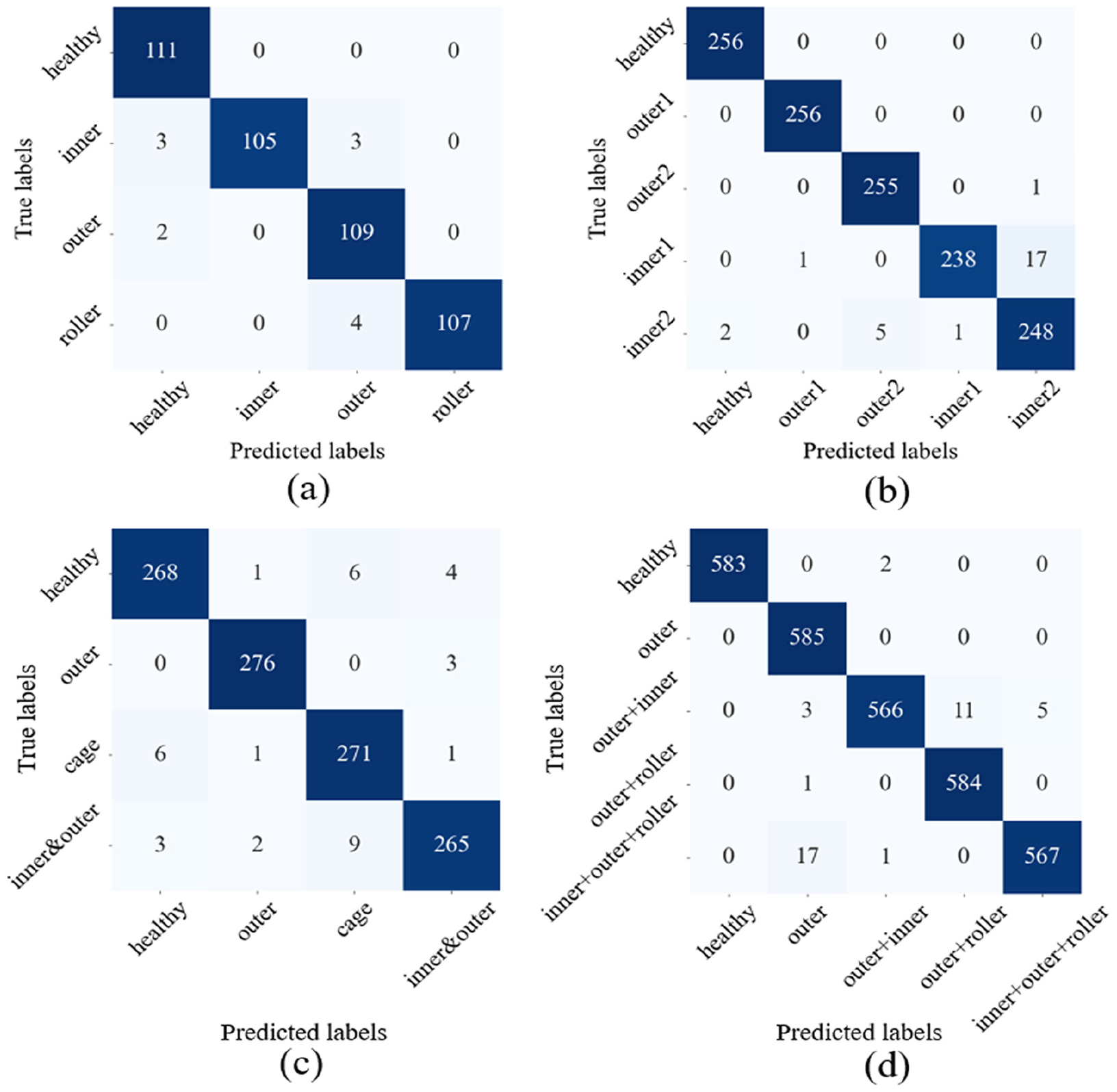
Confusion matrix of training result: (a) confusion matrix for dataset 1, with an accuracy of 97.3%; (b) confusion matrix for dataset 2, with an accuracy of 97.89%; (c) confusion matrix for dataset 3, with an accuracy of 96.77%; and (d) confusion matrix for dataset 4, with an accuracy of 98.63%.

To visually demonstrate the differences between various methods in the feature space, this study employs t-SNE to perform dimensionality reduction on the high-dimensional features extracted by the CNN model. t-SNE is a nonlinear dimensionality reduction method that effectively preserves local neighborhood structures by minimizing the difference between the similarity of data points in high-dimensional space and the corresponding points in low-dimensional space. The t-SNE visualizations clearly reveal the differences in feature distributions between models, facilitating further analysis and interpretation of transfer learning performance in the target task. The high-dimensional features are extracted from the final layer of the CNN model and applied to verify the effectiveness of transfer learning. To ensure the reliability of the results, a comparison is made with a non-transfer model and a model without feature reshaping. For consistency, the number of iterations and training conditions are kept identical across all experiments on the same dataset.

The t-SNE results based on these datasets are presented in Figure 13, comparing the performance of models without feature reshaping, without fine-tuning, and with the proposed method. As shown in Figure 13(a), the model struggles to effectively distinguish inner ring faults from outer ring faults when feature reshaping is not applied. This is due to the prominence of noise in the wavelet images and the lack of distinct features for these two fault types, which interferes with the model’s prediction. Figure 13(b) illustrates the training results without fine-tuning, showing that while the model can classify different faults with a relatively low accuracy of approximately 90%, significant overlap remains between some fault categories. This is because the model without fine-tuning cannot fully leverage the knowledge from the pre-trained model, limiting its classification accuracy. In contrast, Figure 13(c) demonstrates the test results using the proposed method. The t-SNE visualization clearly reveals that the model can distinctly separate the four fault categories, validating the effectiveness of the proposed approach. For dataset 2, the results are similar to those of dataset 1. As shown in Figures 13(d) to (f), the model without feature reshaping and fine-tuning fails to accurately predict certain inner ring and outer ring faults. However, the model applying both feature reshaping and fine-tuning exhibits good result, with more concentrated and clearly separated feature distributions. For dataset 3, due to higher noise levels, the model without feature reshaping struggles to identify any faults, as shown in Figure 13(g). The model without fine-tuning achieves only low accuracy, with notable overlaps in the t-SNE clusters (Figure 13(h)). In comparison, the model employing both feature reshaping and fine-tuning achieves superior results, as illustrated in Figure 13(i). For dataset 4, as shown in Figures 13(j) to (l), without feature reshaping, the model struggles to distinguish between inner race faults and the combined inner + outer race faults. When fine-tuning is not applied, considerable overlap is observed between the outer race fault and its associated compound faults, indicating limited classification accuracy. In contrast, the proposed method achieves clear and distinct clustering, demonstrating its effectiveness and applicability in diagnosing compound faults.

Figure 13.

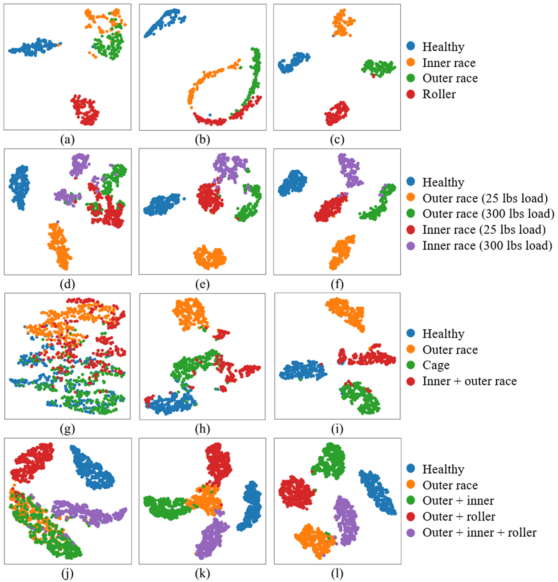
t-SNE analysis: (a–c) dataset 1 under different conditions: without feature reshaping, without fine-tuning, and using the proposed method; (d–f) dataset 2 under the same three conditions; (g–i) dataset 3 under the same three conditions; and (j–l) dataset 4 under the same three conditions. t-SNE: t-distributed stochastic neighbor embedding.

Across these test results, all models consistently distinguish healthy bearing states. This is because the primary features of healthy bearings are concentrated in low-frequency regions, making them less susceptible to noise. The RGB wavelet images of faulty bearings exhibit significant differences from those of healthy states. These t-SNE results confirm the effectiveness of the proposed method across different machines and fault types.

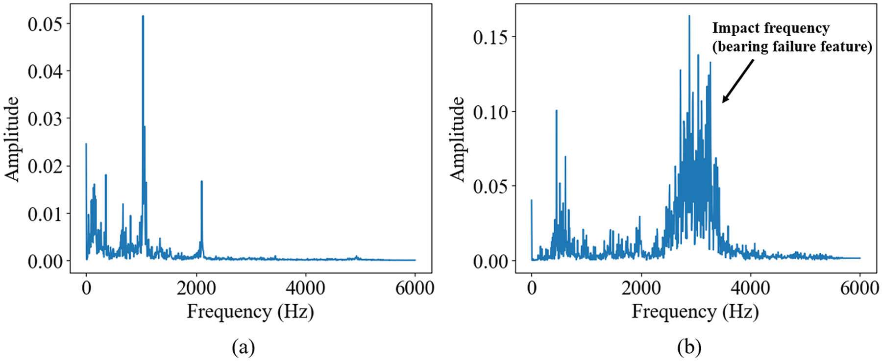
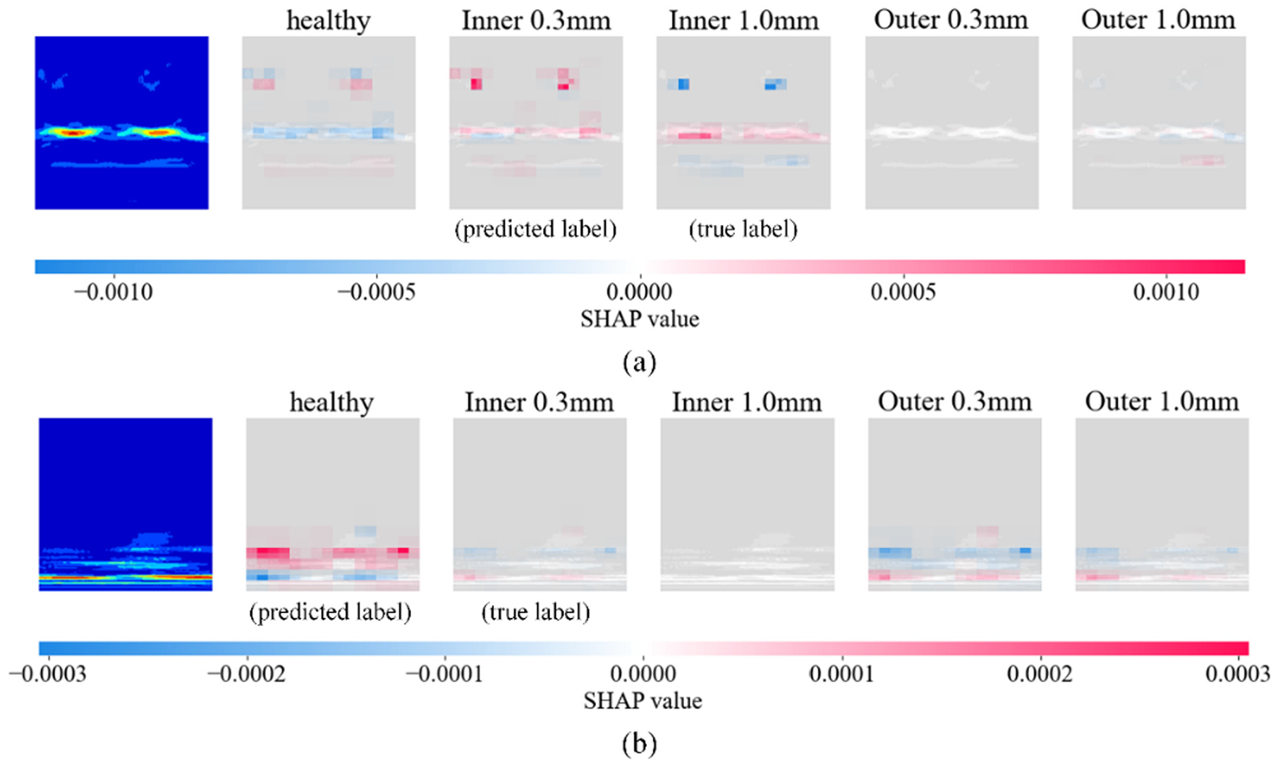
SHAP is employed to analyze the output of the transfer learning model. Figure 14(a) to (d) illustrates the interpretability analysis results of different transfer learning models applied to different datasets in case study 1. In the figure, the color bar represents the magnitude of the SHAP values, where blue indicates negative values and red indicates positive values. Higher SHAP values suggest that the corresponding region has a significant positive contribution to the model’s confidence for a specific label, whereas smaller SHAP values indicate a negative contribution to the label’s confidence to the specific label. In Figure 14(a), the wavelet image for the “healthy” label shows that regions with high SHAP values are concentrated around the low-frequency range near 1 kHz, suggesting that this region plays a crucial role in the model’s prediction of the “healthy” label. In contrast, noise in the high-frequency region is marked in light blue or gray, indicating that these frequency components have low or no weight in the model’s analysis. Similarly, in the wavelet image for the “outer” label in Figure 14(a), regions with high SHAP values (marked in red) are concentrated around 4.2 kHz, whereas noise in the low- and high-frequency regions is assigned lower SHAP values, marked in light blue and gray. Light blue areas have SHAP values that are negative but close to zero, implying a weak negative contribution to the model’s prediction, thus having limited influence on the model’s decision-making. Gray areas indicate that the model has partially recognized and ignored noise, treating it as features with no significant impact on classification.

Figure 14.

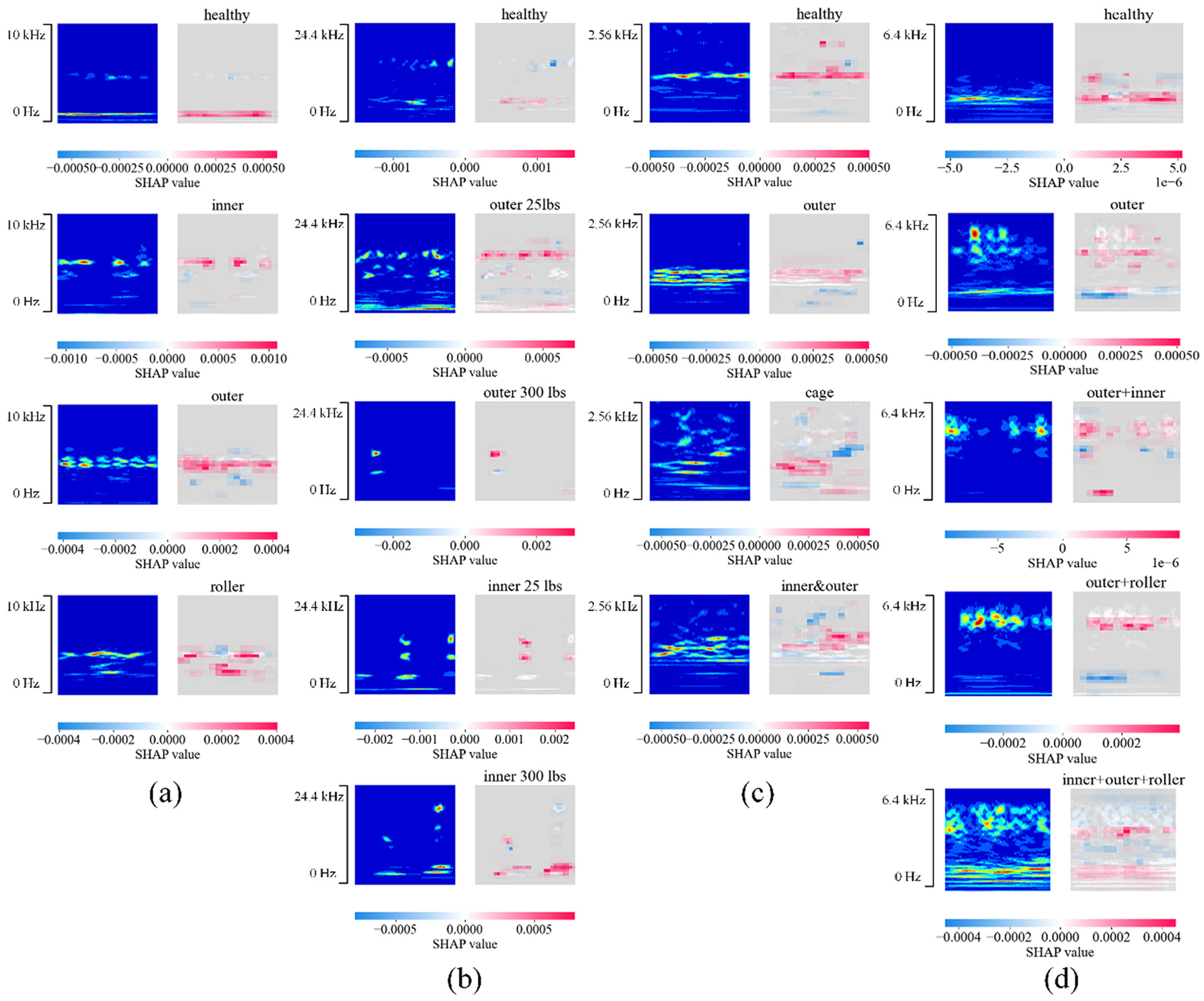
SHAP analysis of case study 1: (a) dataset 1, (b) dataset 2, (c) dataset 3, and (d) dataset 4. SHAP: Shapley Additive Explanation.

By integrating CWT and SHAP interpretability analysis, regions that negatively influence the model’s predictions can be effectively identified, allowing for adjustments to improve model performance. In this case study, regions with low SHAP values generally correspond to noise outside the characteristic frequencies. For instance, in Figure 14(c), certain high-frequency regions above 1600 Hz exhibit low SHAP values, which may interfere with the model’s predictions and reduce accuracy. Through interpretability analysis, filters can be redesigned to reshape features, filtering out high-frequency noise and mitigating its negative impact on the model’s decisions, thereby enhancing performance. For example, after introducing a low-pass filter at 1600 Hz for dataset 3, the model’s accuracy on the test set improved from 96.77 to 98.32%. This improvement is attributed to the low-pass filter reducing the influence of low-SHAP-value frequency components on the model’s predictions. Figure 14(d) presents the SHAP-based interpretability analysis for compound faults, where the regions with high SHAP values align with known fault characteristic frequencies. This indicates that the model is still able to focus on critical feature regions when handling compound fault conditions.

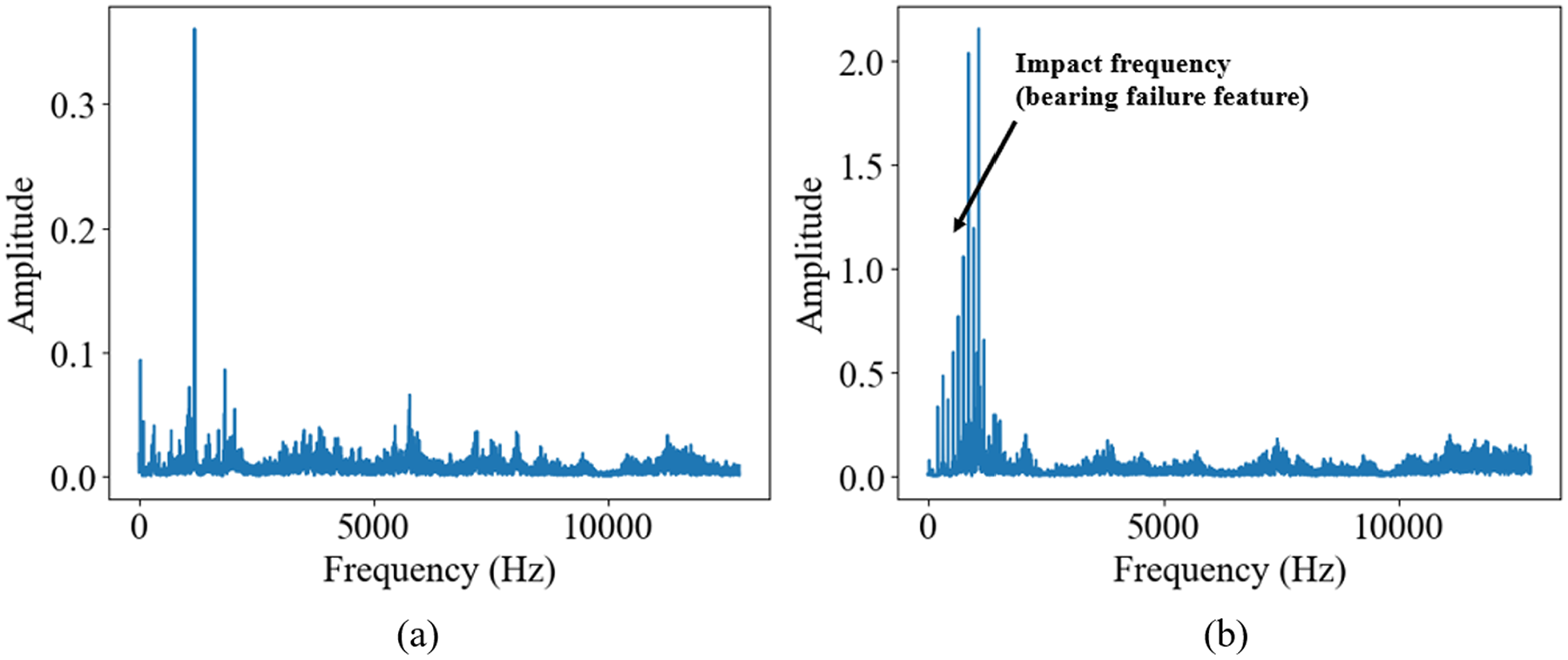
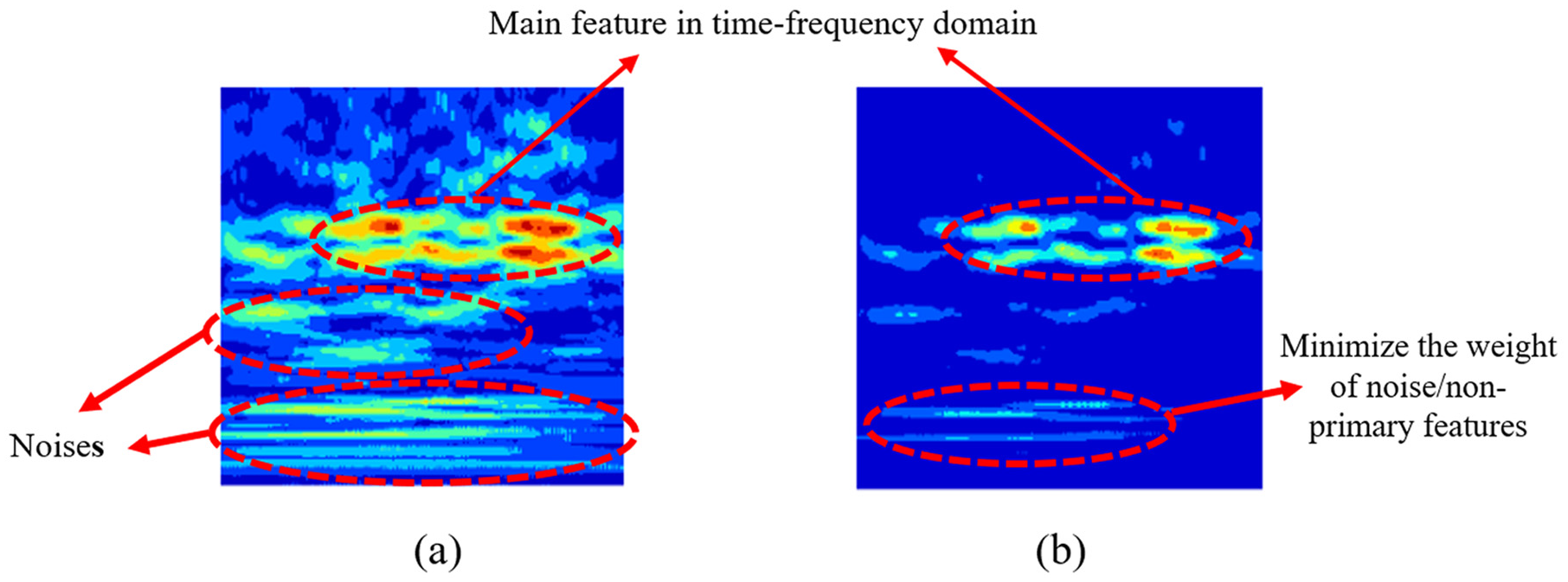
Figure 15 presents the representative SHAP-based interpretability analysis example under three different strategies: the proposed method (Figure 15(a)), without fine-tuning (Figure 15(b)), and without feature reshaping (Figure 15(c)). These comparisons highlight how different transfer strategies influence the model’s attention to fault-related features and classification performance, thereby demonstrating both the occurrence of negative transfer and the effectiveness of feature reshape. Figure 15(a) shows the result obtained using the proposed method, which combines feature reshaping and fine-tuning. The model correctly classifies the input and focuses on the critical frequency region around 4.5 kHz, indicating strong fault recognition capability and good domain adaptability. Figure 15(b) illustrates the case without fine-tuning. Due to the small dataset size and the lack of adaptation to the target domain, the model struggles to distinguish between outer race and roller faults. The SHAP maps of both fault types exhibit high weights in the mid-frequency range, resulting in similar confidence levels and misclassification. This reflects a typical case of negative transfer, where the model fails to adapt effectively to the target domain features. Figure 15(c) reveals another form of negative transfer. When the model is trained directly on the raw signals without feature reshaping, it is able to identify the healthy class but shows considerable confusion among inner race, outer race, and roller faults. The SHAP weights are mostly concentrated in non-informative regions, overlooking key fault frequencies. Different fault classes receive high prediction confidence, leading to unclear classification boundaries. This suggests that signals without feature reshaping lack domain alignment, thereby causing negative transfer. These results demonstrate that without appropriate domain adaptation mechanisms, such as fine-tuning and feature reshaping, transfer learning models not only fail to extract critical features effectively but may also suffer from performance degradation due to feature mismatch. The proposed method mitigates these issues by improving the model’s robustness and generalization capability under complex fault conditions. This finding is further supported by the t-SNE visualization shown in Figure 13.

Figure 15.

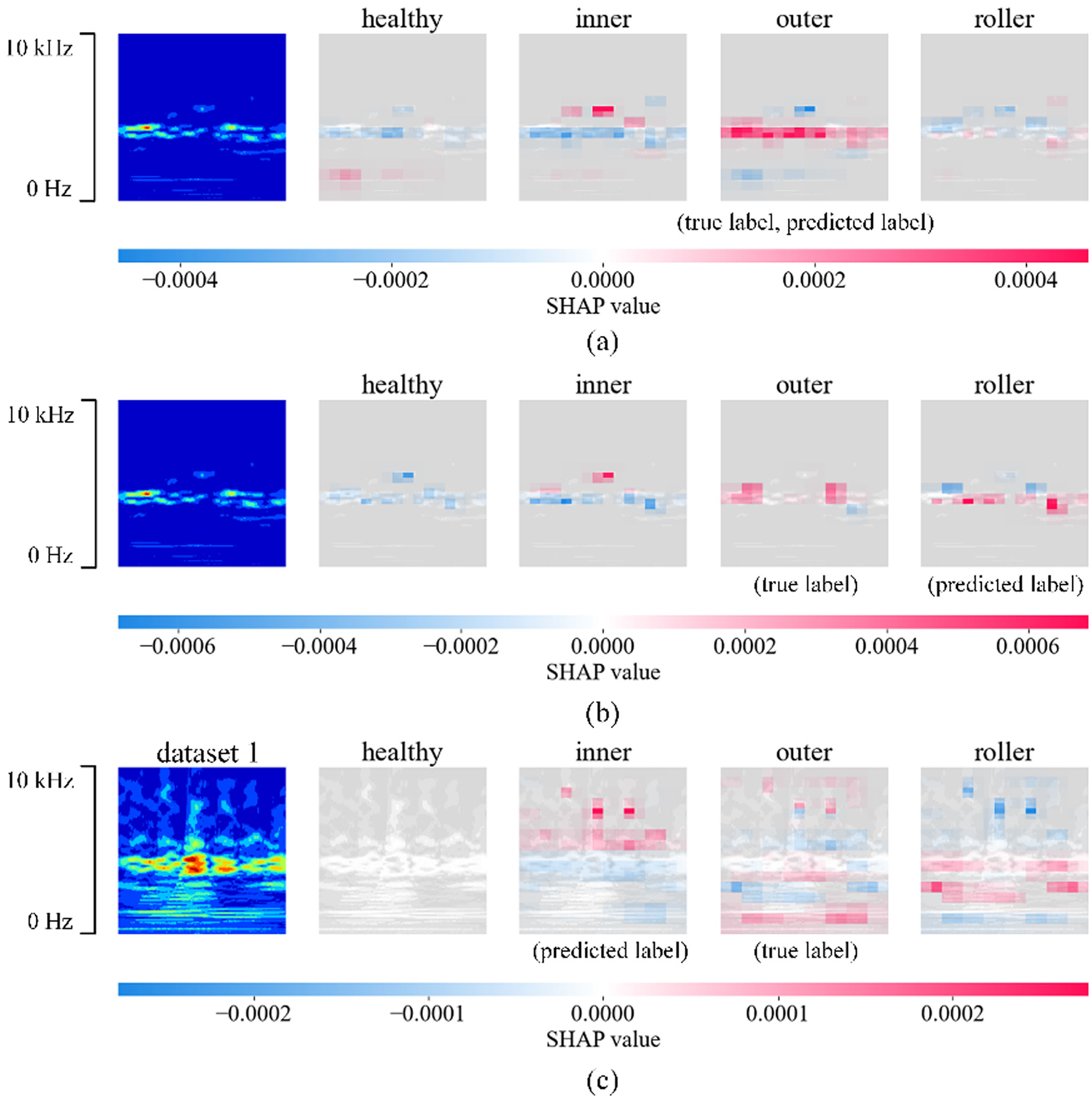
SHAP analysis of case study 1: (a) proposed method, (b) without feature reshape, and (c) without fine-tuning. SHAP: Shapley Additive Explanation.

Case study 2: transfer learning between different signal types

Case study 2 illustrates another application scenario of the proposed transfer learning method, specifically focusing on transfer learning between different signals. This case study utilizes the acoustic signals from the KAIST bearing dataset. The dataset includes 120 s of data collected under normal conditions and 60 s of data under faulty conditions, with a sampling frequency of 51.2 kHz.³⁵ To avoid interference from external noise, the fault data are acquired under no-load conditions. In this study, 1.8 s of data are randomly selected, with 1.2 s used for training and 0.6 s for validation. The acoustic dataset is labeled as dataset 5.

In certain industrial environments, microphones offer an efficient solution due to their ease of installation and low cost, particularly in situations where accelerometers are constrained by hardware limitations or complex operational conditions. Accelerometers typically require direct contact with the equipment, which involves complicated installation processes and may necessitate operational downtime. Furthermore, deploying accelerometers in harsh environments, such as those involving high temperatures, high pressures, or corrosive conditions, can significantly increase both cost and complexity. In contrast, microphones can be installed remotely, collecting acoustic signals in a non-contact manner, thus overcoming these limitations and making them well-suited for monitoring operational equipment or inaccessible areas. Moreover, the acoustic signals from bearings share significant similarities with the vibration signals measured by accelerometers in terms of their generation mechanisms and frequency characteristics. Abnormalities caused by bearing faults often manifest as comparable patterns of change in the time–frequency domain for both acoustic and vibration signals. These similarities provide a robust foundation for transfer learning. In scenarios such as rotary machinery, mechanical vibrations induce anomalies that simultaneously affect both acoustic and vibration signals. The shared frequency characteristics and patterns of these signals can be effectively identified using a unified feature extraction module. By using transfer learning, pre-trained models based on accelerometer data can be fine-tuned for acoustic signals, allowing the model to utilize features learned from accelerometer data. This approach addresses the challenge of limited acoustic signal data, enabling high-performance monitoring even with scarce data. Consequently, this method provides a flexible, cost-effective, and efficient solution for equipment condition assessment in industrial environments.

In line with case study 1, we apply the same preprocessing steps to the acoustic data. Figure 16 shows a comparison of the signals before and after processing. First, spectral analysis is performed on the signals, and the signals are resampled based on their characteristic frequencies. In this case, the original 51.2 kHz acoustic signal is resampled to 10 kHz. Subsequently, the signal is segmented, and each segment is processed using CWT. During this process, the signal amplitude is normalized to prepare it for processing by the CNN. Additionally, a nonlinear transformation is applied to the signal based on its SNR, emphasizing the key frequency features and enhancing the signal’s transferability.

Figure 16.

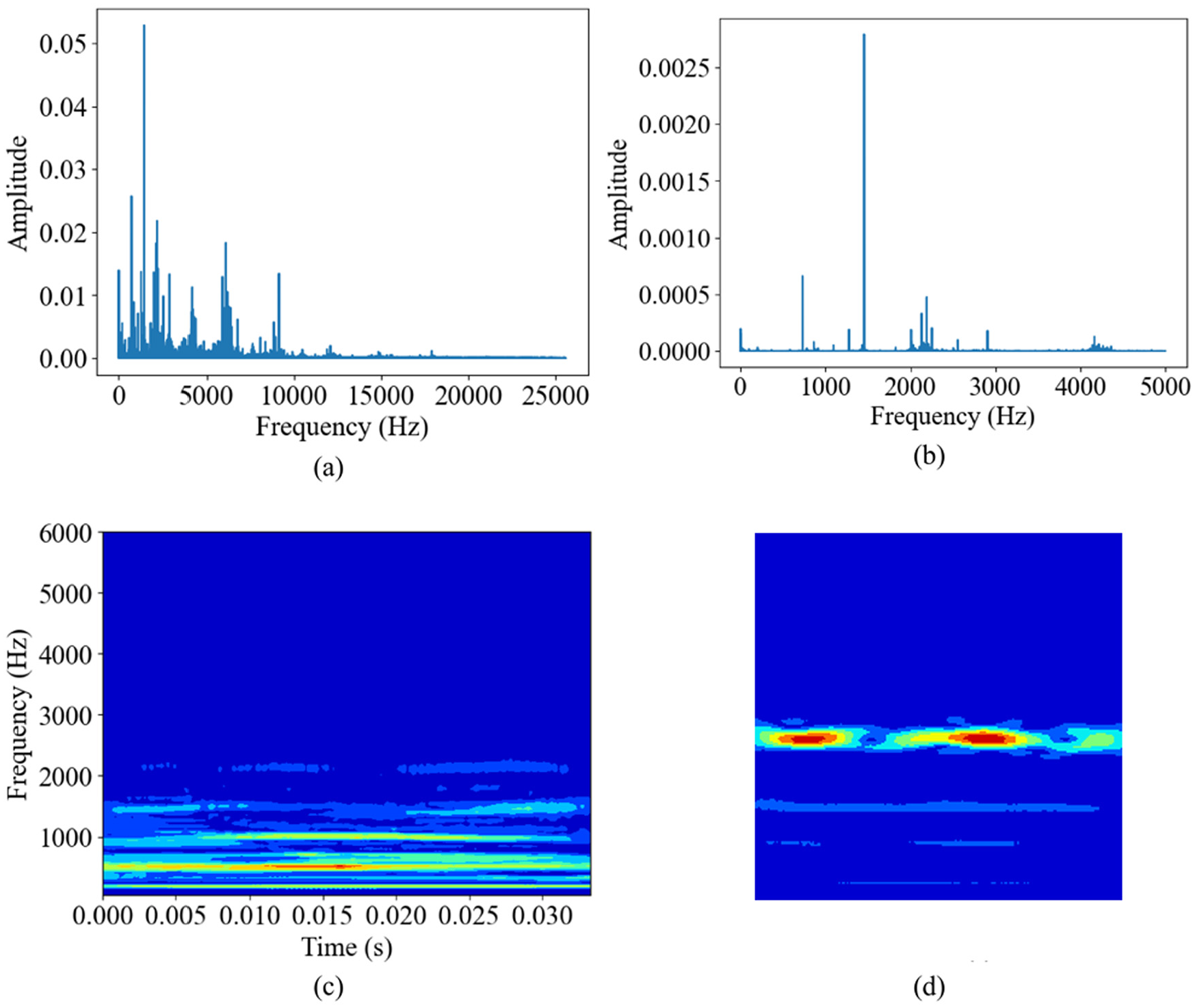
Example of feature reshape: (a) the FFT result of the original signal; (b) the FFT result of the signal after feature reshaping, with the main features concentrated near the center of the spectrum and more prominent amplitude; (c) the time–frequency domain image without feature reshaping, where the image features are difficult for a pre-trained model to recognize; and (d) after feature reshaping based on frequency domain analysis, the main features of the wavelet image become clearer. FFT: fast Fourier transform.

The training environment for case study 2 is the same as that for case study 1. The training and validation accuracies reach 99.66 and 99.31%, respectively. We employ the same approach as in case study 1 to evaluate the transfer learning results. Figure 17 presents the confusion matrix for the acoustic data transfer learning, with a test accuracy of 96.7%. We used the t-SNE method to compare and validate the model’s test results, as shown in Figure 18. It is observed that, without feature reconfiguration, the model struggled to accurately identify fault patterns, leading to cluster confusion. Similarly, without fine-tuning, the model failed to achieve higher accuracy. Only when both feature reconfiguration and fine-tuning are applied did the model generate distinct and well-separated clusters. This is very similar to the results of case study 1.

Figure 17.

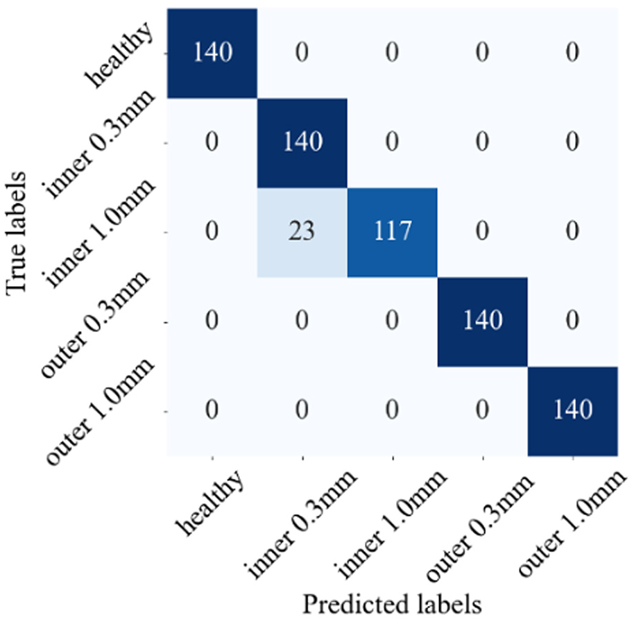
Confusion matrix of case study 2.

Figure 18.

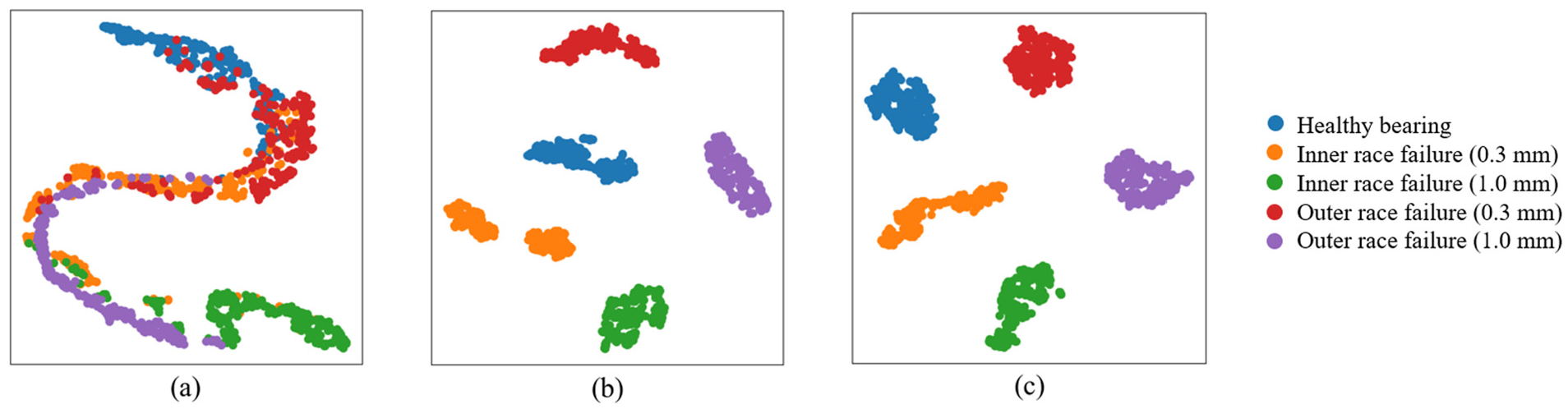
t-SNE analysis of training result of case study 2: (a) without feature reshaping, (b) without fine-tuning, and (c) using the proposed method. t-SNE: t-distributed stochastic neighbor embedding.

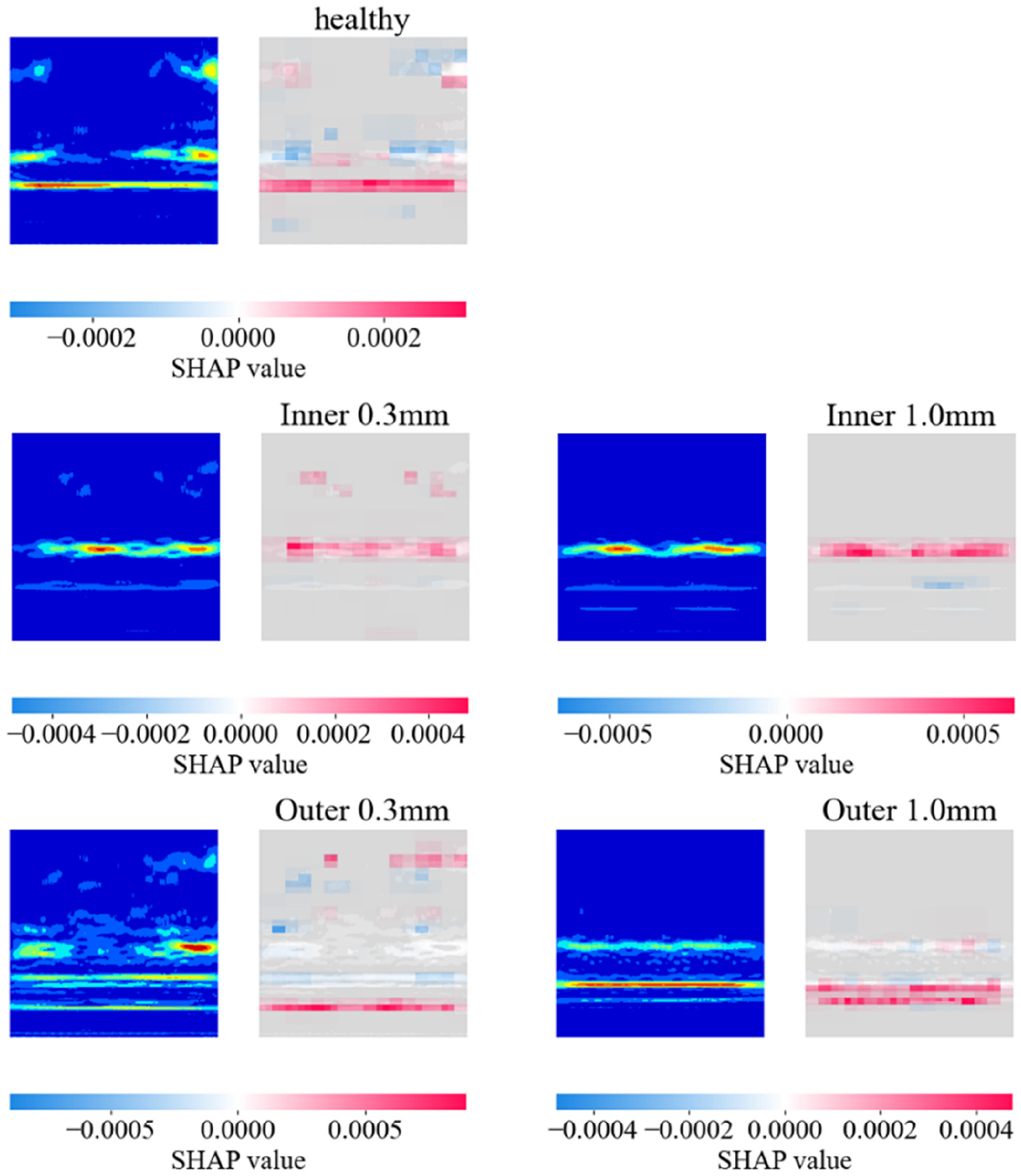
This case study also employs the SHAP to perform interpretability analysis of the model’s performance. The results of transfer learning are presented in Figure 19. As shown in Figure 19, the SHAP values corresponding to each label are relatively high. In certain cases, lower SHAP values can be observed, such as in the high-frequency noise regions of healthy and outer 0.3 mm images. However, since the SHAP values caused by noise are low, they have little impact on the confidence in the correct labels. This indicates that the model successfully learns the acoustic time–frequency patterns corresponding to different fault states. Even though these frequency components are primarily concentrated in the range of approximately 1000–1500 Hz, the model is able to achieve high-accuracy fault classification.

Figure 19.

SHAP analysis of case study 2. SHAP: Shapley Additive Explanation.

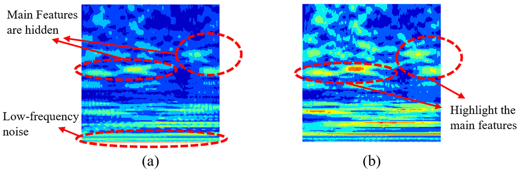
Additionally, SHAP interpretability analysis is conducted for models without fine-tuning and feature reshaping, as shown in Figure 20. Figure 20(a) illustrates the case without fine-tuning. In this scenario, the model suffers from overfitting on small samples, and the similarity between inner 1.0 mm and inner 0.3 mm samples makes it difficult for the model to distinguish between similar patterns or features. Figure 20(b) presents the interpretability analysis results for the model without feature reshaping. In this case, the absence of nonlinear noise transformation and resampling causes the features to concentrate in the lower regions of the image. This prevents the model from effectively identifying features corresponding to different bearing states, leading to error prediction.

Figure 20.

SHAP analysis of case study 2: (a) dataset 2 without fine-tuning and (b) dataset 2 without feature-reshaping. SHAP: Shapley Additive Explanation.

Discussion

Impact of training data scale on model performance

To further evaluate the performance of the proposed method under different training sample sizes, comparative experiments are conducted between the transfer learning model and the non-transfer learning model. For the transfer learning model, the number of training samples is varied from 100 to 800 to simulate data-scarce conditions. For the non-transfer learning model, the training sample size ranged from 250 to 1500. In all experiments across each dataset, the test set is kept consistent to ensure fair comparisons. As shown in Figure 21, the transfer learning model demonstrated higher classification accuracy under small-sample conditions, with particularly pronounced advantages when the number of training samples is below 500. In contrast, the non-transfer learning model required a larger amount of training data to achieve comparable accuracy. These results validate the effectiveness of the proposed method in scenarios with limited training data.

Figure 21.

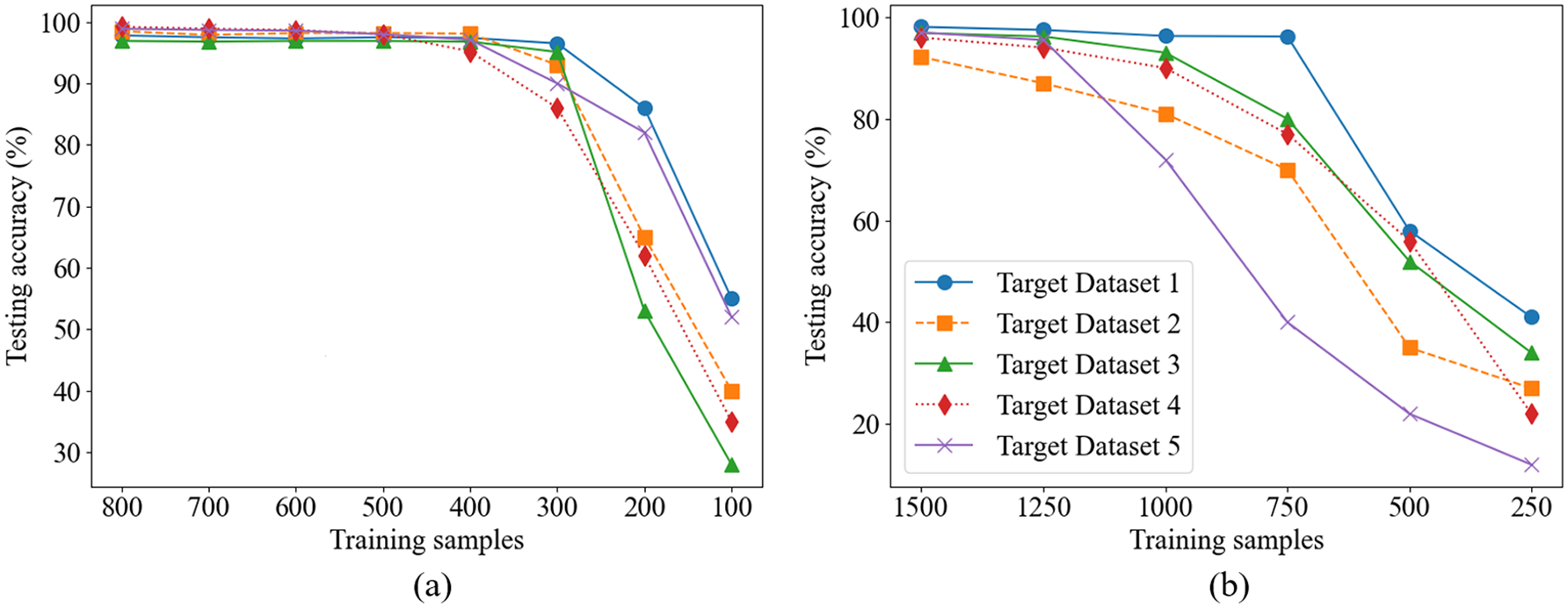
Training data scale and accuracy: (a) transfer learning model and (b) non-transfer learning model.

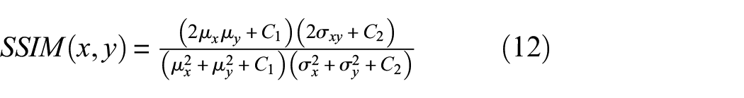
Intra-class consistency

To evaluate the consistency of model predictions within the same fault class, we analyze SHAP attribution maps using two metrics: structural similarity index (SSIM) and cosine similarity (CS). Since SHAP is applied to CWT-based time–frequency images, fault types with distinct frequency patterns are expected to produce similar attribution distributions within the same class. To enhance visual differences and reduce saturation from high-intensity SHAP values, a logarithmic transformation was applied:

\begin{matrix} \tilde{S} (x, y) = \log (1 + S (x, y)) \end{matrix}

(11)

where $\tilde{S} (x, y)$ denotes the original SHAP value at pixel location (x, y). This transformation amplifies differences in low-attribution regions while suppressing the dominance of extremely high values, resulting in a more balanced representation. SSIM evaluates the visual resemblance between images by considering contrast, and structural information, the mathematical expression of SSIM is given by:

\begin{matrix} SSIM (x, y) = \frac{(2 μ_{x} μ_{y} + C_{1}) (2 σ_{xy} + C_{2})}{(μ_{x}^{2} + μ_{y}^{2} + C_{1}) (σ_{x}^{2} + σ_{y}^{2} + C_{2})} \end{matrix}

(12)

where $μ_{x}$ , $μ_{y}$ are mean intensity values, $σ_{x}^{2}$ , $σ_{y}^{2}$ are the variances, reflecting contrast, and $σ_{xy}$ is the covariance of images x and y; C₁ and C₂ are constants to stabilize the division. An SSIM value closer to 1 means the two images are more similar. Cosine similarity is used to measure the consistency of the SHAP attribution maps in terms of direction after flattening. It is calculated as

\begin{matrix} CosSim = \frac{A \cdot B}{∥ A ∥ \cdot ∥ B ∥} . \end{matrix}

(13)

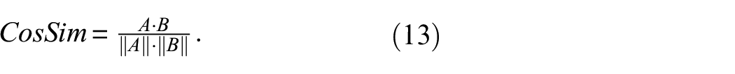
where A and B represent the normalized SHAP vectors. A cosine similarity value closer to 1 indicates that the model focuses on similar patterns across samples of the same class.

Pairwise similarities were computed between samples within each fault class. For each class, 100 pairs of SHAP images are randomly selected to calculate inter-class similarity, SSIM and CS are averaged. Results show average SSIM values above 0.7 and cosine similarities exceeding 0.8 across all datasets, indicating stable and consistent attribution patterns, as shown in Figure 22.

Figure 22.

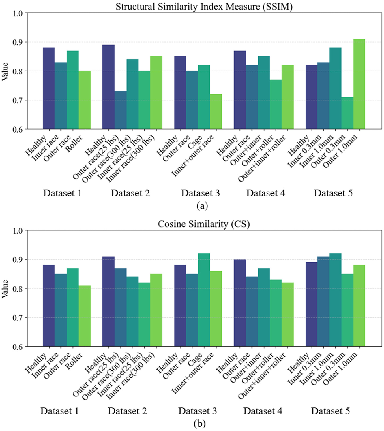
SHAP intra-class consistency: (a) structural similarity index measure and (b) cosine similarity.

Inter-class separability

To assess the model’s ability to distinguish between different fault types, we evaluated the structural dissimilarity of SHAP maps between classes using SSIM. For each fault type, a mean SHAP diagram was generated by averaging the log-transformed attribution maps of all samples in the class. This reduces noise and highlights common attribution patterns.

SSIM was then calculated between each pair of mean SHAP diagrams, forming a similarity matrix that reflects the distinctiveness of each fault category. Compared to cosine similarity, SSIM is more sensitive to local luminance, contrast, and spatial structure, making it more suitable for evaluating time–frequency-based SHAP maps.

The resulting SSIM matrix in Figure 23 shows low similarity scores between different fault classes, indicating clear structural differences in their SHAP patterns and confirming that the model effectively separates different fault categories in terms of learned feature importance.

Figure 23.

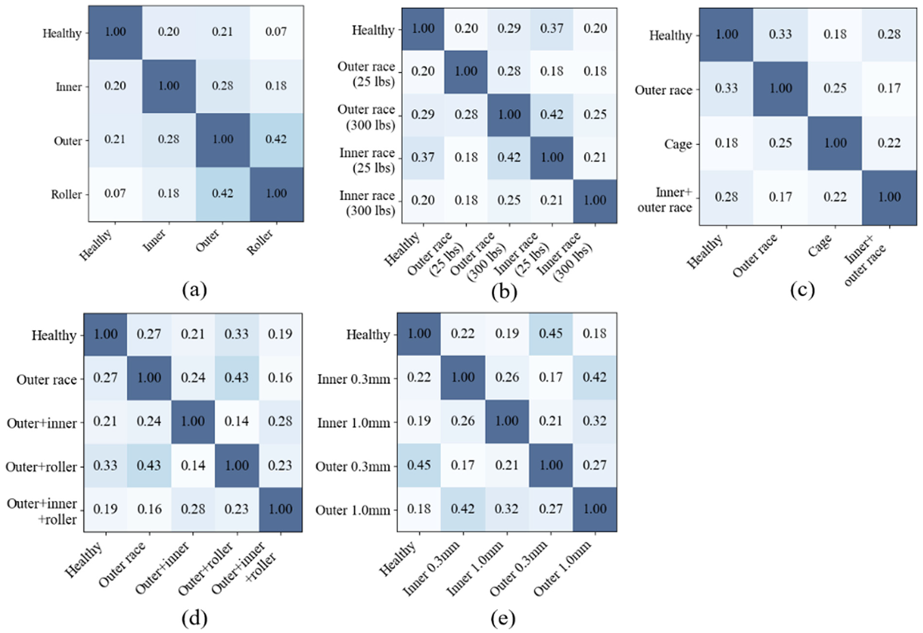
SHAP inter-class separability: (a)–(e) represent the results for datasets 1–5, respectively. SHAP: Shapley Additive Explanation.

Conclusion

This study proposes an interpretable transfer learning method for bearing fault diagnosis that is applicable across different fault types, mechanical systems, and signal types. By integrating CWT-based time–frequency representations with a feature reshaping strategy and fine-tuning, the method enhances domain similarity and signal clarity, enabling effective transfer learning under small-sample conditions.

Experimental results from two case studies validate the robustness of the method. In the first, data from different bearing systems are used, while the second uses acoustic signals. In both cases, the method achieves high diagnostic accuracy with limited target data, confirming its generalizability. The model also performs well in compound fault scenarios, demonstrating its ability to handle more complex conditions.

Interpretability analysis using SHAP and t-SNE further supports the effectiveness of the proposed strategy. SHAP analysis reveal that high SHAP values are concentrated in key time–frequency regions related to faults, highlighting the model’s ability to focus on critical signal features while minimizing the impact of noise. This focused feature extraction further validates the importance of feature reshaping and fine-tuning in enhancing the model’s performance. Moreover, SHAP also enables negative transfer analysis of the model, allowing the identification of regions in the frequency band with low SHAP values, which correspond to features that the model struggles to recognize, or areas influenced by noise. By optimizing filters in these frequency bands, the model’s performance can be further improved, enhancing its robustness and diagnostic accuracy in complex signal environments. This method exhibits strong scalability and can be applied to other datasets, such as ultrasound signals or cutting force signals.

Footnotes

Author contributions

Zhicong Rong: writing—original draft, visualization, validation, software, methodology, investigation, formal analysis. Jihyun Lee: writing—review and editing, supervision.

Declaration of conflicting interests

The author(s) declared no potential conflicts of interest with respect to the research, authorship, and/or publication of this article.

Funding

The author(s) disclosed receipt of the following financial support for the research, authorship, and/or publication of this article: This work is supported by the GN Corporations Inc., Natural Sciences and Engineering Research Council of Canada Alliance Grants, and Campus Alberta Small Business Engagement Program.

ORCID iD

Jihyun Lee

References

Zhang

Wang

, et al. Deep learning algorithms for bearing fault diagnostics—a comprehensive review. IEEE Access 2020; 8: 29857–29881.

Bhuiyan

Uddin

Deep transfer learning models for industrial fault diagnosis using vibration and acoustic sensors data: a review. Vibration 2023; 6(1): 218–238.

Guo

A review on prognostics methods for engineering systems. IEEE Trans Reliab 2020; 69(3): 1110–1129.

Rai

Upadhyay

SH.

A review on signal processing techniques utilized in the fault diagnosis of rolling element bearings. Tribol Int 2016; 96: 289–306.

Yan

Yang

, et al. A review on rolling bearing fault signal detection methods based on different sensors. Sensors 2022; 22(21): 8330.

Tang

Gao

Wang

, et al. A novel intelligent fault diagnosis method for rolling bearings based on Wasserstein generative adversarial network and convolutional neural network under unbalanced dataset. Sensors 2021; 21(20): 6754.

Wang

Sun

Zhu

, et al. A fault diagnosis method based on an improved diffusion model under limited sample conditions. PLoS One 2024; 19(9): e0309714.

Song

Liu

Wang

Rolling bearing fault diagnosis in electric motors based on IDIG-GAN under small sample conditions. Meas Sci Technol 2024; 35(10): 106105.

Zheng

Song

Wang

, et al. Data synthesis using dual discriminator conditional generative adversarial networks for imbalanced fault diagnosis of rolling bearings. Measurement 2020; 158: 107741.

10.

Chow

M-Y

Tipsuwan

, et al. Neural-network-based motor rolling bearing fault diagnosis. IEEE Trans Ind Electron 2000; 47(5): 1060–1069.

11.

Deep learning based approach for bearing fault diagnosis. IEEE Trans Ind Appl 2017; 53(3): 3057–3065.

12.

Sarker

IH.

Deep learning: a comprehensive overview on techniques, taxonomy, applications and research directions. SN Comput Sci 2021; 2(6): 420.

13.

Lin

, et al. A multi-stage semi-supervised learning approach for intelligent fault diagnosis of rolling bearing using data augmentation and metric learning. Mech Syst Signal Process 2021; 146: 107043.

14.

Wang

Dong

Wang

, et al. Limited fault data augmentation with compressed sensing for bearing fault diagnosis. IEEE Sens J 2023; 23(13): 14499–14511.

15.

Zhang

Ding

, et al. Intelligent rotating machinery fault diagnosis based on deep learning using data augmentation. J Intell Manuf 2018; 31(2): 433–452.

16.

Kulevome

DKB

Wang

Cobbinah

, et al. Effective time-series data augmentation with analytic wavelets for bearing fault diagnosis. Exp Syst Appl 2024; 249: 123536.

17.

Han

Jeong

, et al. Bearing fault diagnosis based on multiscale convolutional neural network using data augmentation. J Sens 2021; 2021(1): 6699637.

18.

Chen

Yang

Xue

, et al. Deep transfer learning for bearing fault diagnosis: a systematic review since 2016. IEEE Trans Instrum Meas 2023; 72: 1–21.

19.

Zhao

Zhang

, et al. Applications of unsupervised deep transfer learning to intelligent fault diagnosis: a survey and comparative study. IEEE Trans Instrum Meas 2021; 70: 1–28.

20.

Yang

Zhang

Jiang

Mechanical fault diagnosis based on deep transfer learning: a review. Meas Sci Technol 2023; 34(11): 112001.

21.

Qian

Zhu

Shen

, et al. Deep transfer learning in mechanical intelligent fault diagnosis: application and challenge. Neural Process Lett 2022; 54(3): 2509–2531.

22.

Huang

, et al. A perspective survey on deep transfer learning for fault diagnosis in industrial scenarios: theories, applications and challenges. Mech Syst Signal Process 2022; 167: 108487.

23.

Zhang

Qin

, et al. A systematic review of deep transfer learning for machinery fault diagnosis. Neurocomputing 2020; 407: 121–135.

24.

Kim

Lee

, et al. A domain adaptation with semantic clustering (DASC) method for fault diagnosis of rotating machinery. ISA Trans 2022; 120: 372–382.

25.

Chen

Gryllias

Intelligent fault diagnosis for rotary machinery using transferable convolutional neural network. IEEE Trans Ind Inform 2020; 16(1): 339–349.

26.

Deng

Huang

, et al. A double-layer attention based adversarial network for partial transfer learning in machinery fault diagnosis. Comput Ind 2021; 127: 103399.

27.

Peng

Shao

Yan

, et al. A systematic review on interpretability research of intelligent fault diagnosis models. Meas Sci Technol 2024; 36: 012009.

28.

Sun

Cao

Wang

, et al. An interpretable anti-noise network for rolling bearing fault diagnosis based on FSWT. Measurement 2022; 190: 110698.

29.

Oliveira

RMA

Sant’Anna

ÂMO

da Silva

PHF

. Explainable machine learning models for defects detection in industrial processes. Comput Ind Eng 2024; 192: 110214.

30.

Huang

Tao

Zhao

, et al. Graph structure embedded with physical constraints-based information fusion network for interpretable fault diagnosis of aero-engine. Energy 2023; 283, 2023: 129120.

31.

Case Western Reserve University. Bearing data center. Case Western Reserve University [Online], https://engineering.case.edu/research/ndcl/data-sets-bearing-datacenter (2003, accessed 1 Sepetember 2024).

32.

Lee

Qiu

Lin

and Rexnord Technical Services. Bearing data set. NASA prognostics data repository, Ames Research Center, Moffett Field, CA: IMS, University of Cincinnati, 2007.

33.

Machinery Failure Prevention Technology Society (MFPT). MFPT bearing data set [Online], https://www.mfpt.org/fault-data/ (2012, accessed 1 Sepetember 2024).

34.

Wang

Lei

. A hybrid prognostics approach for estimating remaining useful life of rolling element bearings. IEEE Transactions on Reliability 2020; 69(1): 401–412.

35.

Ding

Qin

Wang

, et al. Evolvable graph neural network for system-level incremental fault diagnosis of train transmission systems. Mech Syst Signal Process 2024; 210: 111175.

36.

Jung

Kim

Yun

, et al. Vibration, acoustic, temperature, and motor current dataset of rotating machine under varying operating conditions for fault diagnosis. Data Brief 2023; 48: 109049.

37.

Kristoffersen

Deep transfer learning for failure prediction across failure types. Comput Ind Eng 2022; 172: 108521.

38.

Yan

Gao

Chen

Wavelets for fault diagnosis of rotary machines: a review with applications. Signal Process 2014; 96: 1–15.

39.

Simonyan

Zisserman

. Very deep convolutional networks for large-scale image recognition. In: 3rd International Conference on Learning Representations (ICLR 2015), San Diego, CA, 7–9 May 2015, pp. 1–14. Computational and Biological Learning Society.

40.

Liu

Deng

. Very deep convolutional neural network based image classification using small training sample size. In: 3rd IAPR Asian Conference on Pattern Recognition (ACPR), Kuala Lumpur, Malaysia, 3–6 November 2015, pp. 730–734. IEEE.

41.

Lundberg

Lee

S-I

. A unified approach to interpreting model predictions. In: 31st International Conference on Neural Information Processing Systems (NeurIPS), Long Beach, CA, 4–9 December 2017, pp. 4768–4777. Curran Associates Inc.

An interpretable transfer learning method for bearing diagnosis across different systems,faults,and signal types

Abstract

Keywords

Introduction

Dataset description

Development of the proposed transfer learning method

Time–frequency methods

Convolution neural network and training

Proposed framework for transfer learning

Data preprocessing

Shapley additive explanations

Validation through case studies

Case study 1: transfer learning between different machines and faults

Case study 2: transfer learning between different signal types

Discussion

Impact of training data scale on model performance

Intra-class consistency

Inter-class separability

Conclusion

Footnotes

Author contributions

Declaration of conflicting interests

Funding

ORCID iD

References