
Abstract
Deep learning networks have been widely applied in signal processing for structural health monitoring, enabling a more comprehensive and automated analysis. However, existing research primarily focused on identifying faulty signals and the presence of defects, with few studies addressing defect quantification. Particularly, previous research on invisible defects has predominantly targeted delamination in carbon fibre-reinforced polymer and fibre-reinforced polymer-concrete, with limited attention given to the tiling systems. Although techniques have been developed for identifying debonding in such structures, research on debonding quantification has been limited due to the challenges of analysing and differentiating complex vibration signals. This study thus aims to develop an automated system for classifying the debonding size of tile panels based on their vibration responses. The proposed approach involved transforming the waveform data into scalograms, followed by augmentation to prepare the dataset for network training. An ad-hoc convolutional neural network was designed to categorise the vibration data into three classes that represent different ranges of debonding sizes. The network training involves both simulated and experimental data, achieving high accuracy in predicting simulated data while having relatively lower accuracy for experimental data. This can be attributed to the discrepancies between simulated and experimental data, as well as the challenges in identifying cases at the boundaries of two adjacent classes. The limited size of the experimental dataset may also have constrained the performance of the trained network.
Keywords
Introduction
Adhesive ceramic tilling systems (ACTs) have emerged as a popular cladding option for contemporary civil infrastructures, owing to their functional and aesthetic benefits. However, the effectiveness of ACTs significantly relies on the quality of materials, workmanship and execution compared to alternatives such as cementitious render or stone.1–3 Among the various anomalies found in ACTs, interfacial debonding stands out as the most critical defect due to the potential risk to pedestrians of falling tiles. 4 Debonding occurs as a result of differential shrinkage and thermal expansion among the three primary components of ACTs – tile, adhesive and substrate. Interfacial traction leads to debonding at either the tile-to-adhesive or adhesive-to-substrate interfaces. 5 Subsequent to the initial occurrence of debonding, the rate of degradation accelerates due to water penetration. 6 This underscores the importance of conducting regular inspections on ACTs to identify interfacial debonding promptly and prevent potential accidents.
There have been various non-destructive testing (NDT) techniques developed for inspecting ACTs, such as infrared thermography (IRT) and tap testing.7–9 IRT has been used for the detection of interfacial defects on a large scale, owing to its capability of rapid scanning and immediate visualisation of anomalies. However, its dependency on specific conditions and equipment limits its practicality in field applications. 10 Tap testing is the most popular technique applied on-site due to its cost-effectiveness. 11 It is understood that the vibration characteristics of a structure are influenced by its structural properties, geometry and boundary conditions, all of which may change over time. Consequently, the transient fluctuations in vibration responses often display notable statistical variations, which offer valuable insights into the structural integrity conditions. Past studies have predominantly focused on identifying the presence of debonding, with limited emphasis on quantifying its severity.12,13 This could be attributed to the challenges in interpreting complex vibration responses and identifying relevant features indicative of defects.
With the advancement of artificial intelligence (AI), deep learning algorithms, particularly convolutional neural network (CNN), have been extensively applied in structural health monitoring (SHM). This is owed to their ability to identify data patterns that may not be evident through conventional assessment methods. SHM systems rely on various sensors to collect data from the target structure, enabling the assessment of the integrity and performance. A notable application of CNNs in SHM is the detection of data anomalies caused by sensor faults, harsh environments and other factors. In some studies, researchers have directly used acceleration data collected by sensors to train 1D-CNNs, which have been proven effective in identifying anomalous data.14,15 In other applications, the raw data was pre-processed and transformed into images, where 2D-CNNs were employed to recognise anomalies.16,17 Tang et al. 18 proposed to convert the acceleration data from a bridge into dual-channel images by integrating time- and frequency-domain plots. In another practice, Gramian angular field (GAF) images transformed from the frequency-domain information of the acceleration data were used for analysis. 19 Both trained 2D-CNN models demonstrated high efficiency and accuracy in detecting multi-pattern anomalies.
There are also many studies that have used CNNs to detect defects in structures by analysing sensor data. Some researchers used raw waveforms as inputs for 1D-CNN training, which successfully detected surface defects such as mass addition and notches on aluminium plates and beams.20–22 Du et al. proposed integrating long short-term memory (LSTM) with CNN to classify the impact damage in carbon fibre-reinforced polymers (CFRPs) into minor, intermediate and severe. 23 Using delay-and-sum (DAS) images generated from guided wave imaging (GWI) algorithms, holes in aluminium plates were successfully localised and quantified by a CNN model. 24 By converting the sound signals during the hammer test into spectrograms, a 2D-CNN was successfully trained to identify interfacial debonding between the fibre-reinforced polymer (FRP) and concrete. 25 In a similar approach, Schackmann et al. 26 used spectrograms to detect and quantify structural abnormalities and fatigue damage in CFRP. Scalograms derived from Lamb wave signals were also used to train CNN models for the purpose of detecting and locating delamination in CFRP. 27 Delamination in laminated composites was successfully classified into healthy and two delamination states using a CNN trained with scalograms. 28
Both 1D- and 2D-CNNs have shown effectiveness in various SHM applications, showcasing their versatility in addressing complex challenges. Notably, 1D-CNNs are more effective as they process raw data directly, reducting signal pre-processing time and facilitating real-time applications. 29 Yet in many practical scenarios, there is often a need to process data from multiple sensors, in which case, 2D-CNNs would be a more suitable option. 30 On the other hand, CNNs are designed to recognise patterns in two-dimensional space, which naturally aligns with the structures in images. Converting 1D signals into 2D or 3D images often yields additional information that might otherwise be lost when using the raw signal directly.
Current research has predominantly concentrated on the diagnosis of faulty signals or the qualification of defects, there has been limited progress in the quantification of defect sizes through the application of neural networks. Furthermore, past studies have primarily focused on visible surface defects such as holes, notches and mass additions. The investigation of invisible delamination has been limited to CFRP and FRP-concrete, where the interlayers are quite thin and the epoxy resin between layers is generally considered isotropic. In contrast, ACTs feature thick and heterogeneous tile-mortar layers. The structural and material disparity fundamentally leads to unique stress distribution and failure mechanisms, necessitating ad-hoc approaches tailored to ACTs. While there have been studies employing CNNs to recognise surface defects such as cracks on ceramic tiles, the application of CNNs to detect invisible interfacial debonding in ACTs remains highly limited.31–33
This study aims to develop an automated system for classifying the debonding sizes in ACTs based on their vibration responses by employing deep learning algorithms. An ad-hoc CNN was developed and trained using a comprehensive database comprising both simulated damage scenarios and experimental testing results. Before inputting into the network, the raw vibration responses were first transformed into scalograms to preserve more information in both the time- and frequency-domains. The performance of the trained network was validated by accurate prediction on both simulated and experimental data, which were effectively classified into corresponding debonding sizes.
Methodology
It is understood that, under impact conditions, healthy regions of ACTs act as rigid thick plates with several layers fully bonded together, while debonded regions behave as flexible thin plates due to reduced effective thickness and stiffness. 12 This difference affects the vibration responses, as the impact energy would be transferred to the flexible body in the form of structural vibrations. By evaluating these characteristic changes in vibration responses, the debonding could be effectively detected and assessed.
This study adopts an ACT model following the previous work, 34 where four identical tile panels are attached to a concrete base with mortar as shown in Figure 1. One of them is defect-free, while the other three have debonding of certain sizes (e.g., d1–d3 in the figure) across the entire thickness of the mortar layer at random positions. While the current study employs circular debonding for simplicity and consistency between simulation and experiments, the underlying mechanism is not inherently dependent on the specific shape or pattern of the defect. Any type of debonding introduces localised changes in structural properties that influence vibration responses in a detectable manner. The vibration of the ACT is stimulated by hammer impact at the tile centre, and the resulting in-plane surface displacements at the centres of the four quadrants are collected for analysis. This one-excitation multiple-detection approach efficiently examines the entire tile area with a single test, providing sufficient information for debonding assessment. Therefore, each damage scenario has four sets of vibration responses that will be used to quantify the debonding. These responses will be processed subsequently for networking training, validating, or testing.
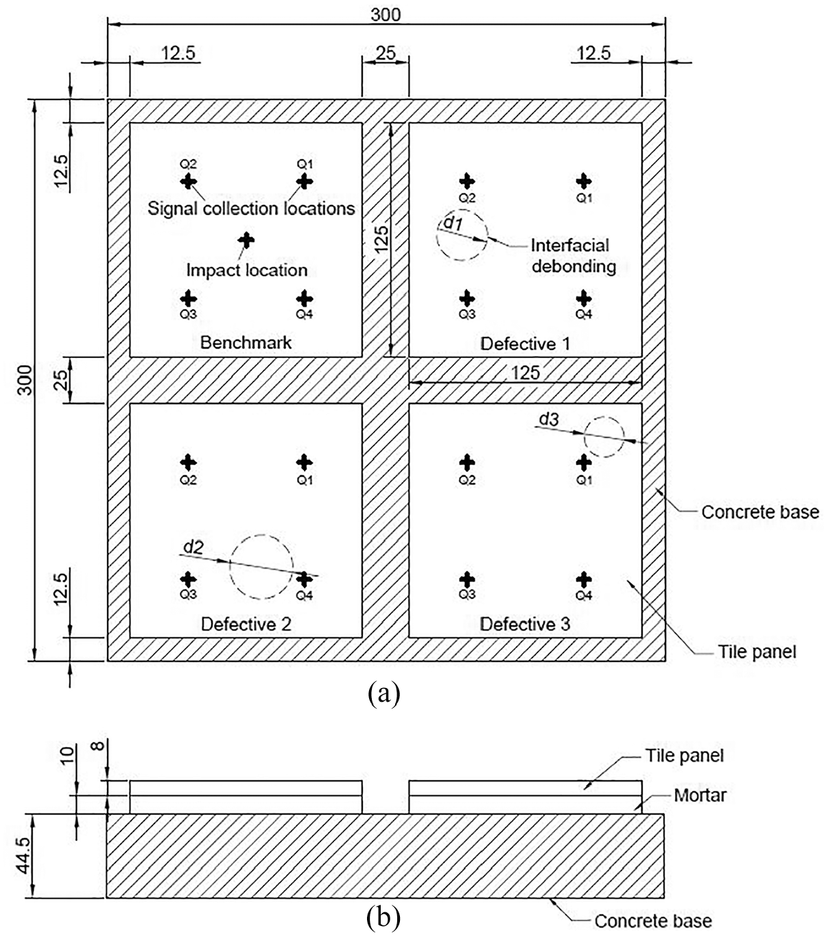
ACT configuration with dimensions in mm from top view (a) and side view (b).
The schematic and workflow of the proposed method are shown in Figure 2, which consists of two main phases: data pre-processing and CNN training. The raw data refers to the collected displacements from the tile surface, obtained through either numerical simulation or experimental testing. Four pieces of waveforms obtained for each damage scenario are converted into scalograms using a continuous wavelet transform (CWT), and then seamlessly combined into a single image representing each individual damage case. With the aim of diversifying the dataset, data augmentation is employed by altering the arrangements of the scalograms from the four quadrants. The augmented dataset is subsequently fed into the CNN, which classifies it into three classes: C1, C2 and C3, where C1 represents defects with a diameter smaller than 20 mm, C2 for those ranging from 20 to 30 mm and C3 for those greater than 30 mm. For better network performance, a large volume of training database is preferred, which is mainly achieved by abundant damage scenarios from numerical simulation. Real-world experimental data will also be integrated to validate and improve the model. The details of each step in the proposed methodology will be presented in the subsequent sections.
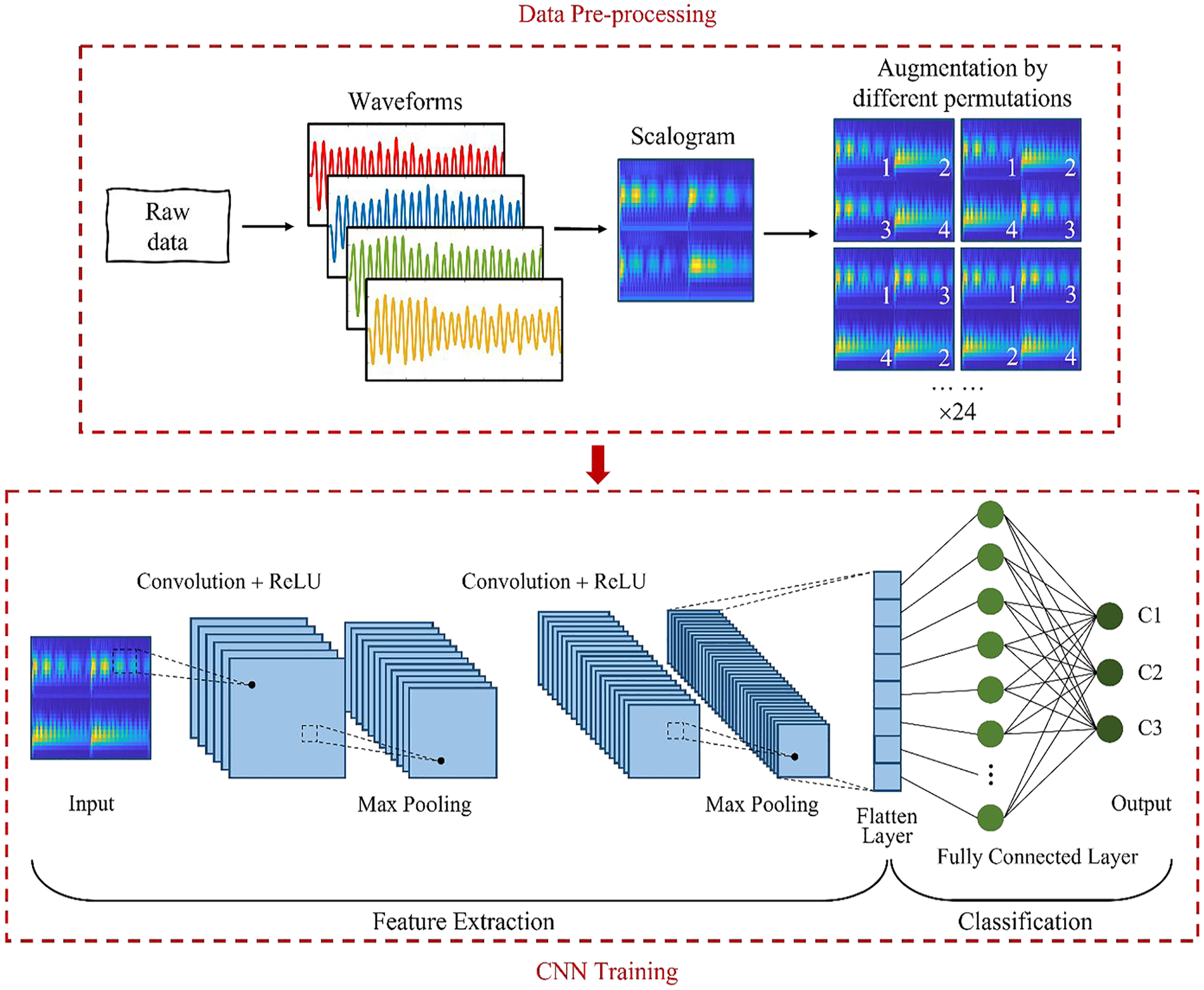
Schematic and workflow of the proposed method for automatic debonding quantification.
Data acquisition
Numerical modelling
Abaqus/Explicit was used to simulate the vibration responses of the four-panel ACT under impact load (Figure 3(a)). The material properties of the tile, mortar and concrete are listed in Table 1. The interfacial debonding was simulated by intentionally removing a circular area across the entire thickness of the mortar layer (Figure 3(b)). This area is not attached to either the tile or the concrete base, thus replicating a debonding. This configuration was deliberately designed to closely match the experimental setup, ensuring consistency in the representation of the debonding defect. It is noteworthy that, in real life, the debonded mortar often remains in place but loses contact with either the tile or the substrate. This, however, still reduces the effective thickness of the structure and alters its vibration responses. Although the configuration used in this study does not fully replicate reality complexities, it is capable of capturing key aspects of the debonding phenomenon and providing a simplified and controlled representation of debonding.
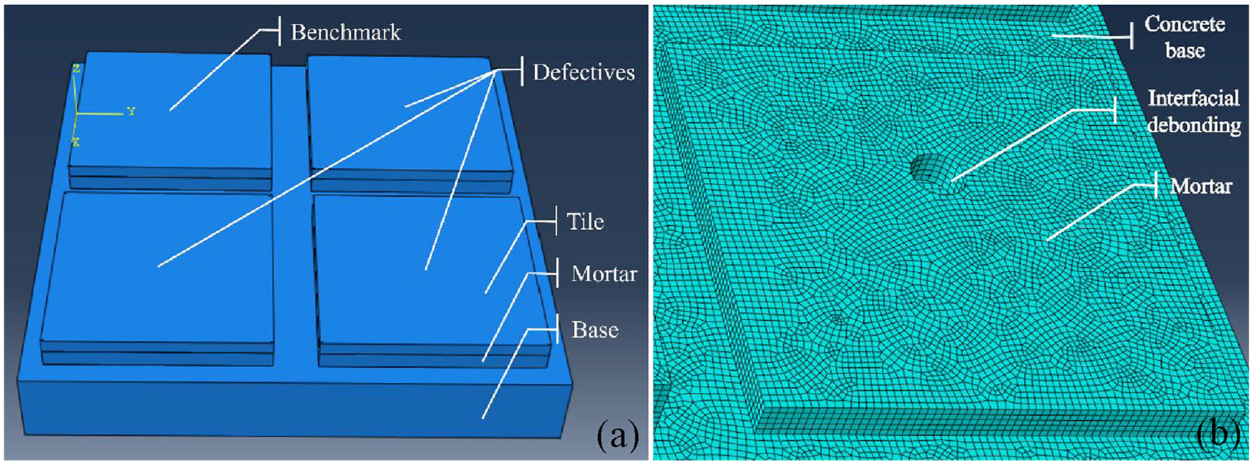
Numerical model of the ACT (a) and the meshes (b).
Material properties used for numerical simulation.
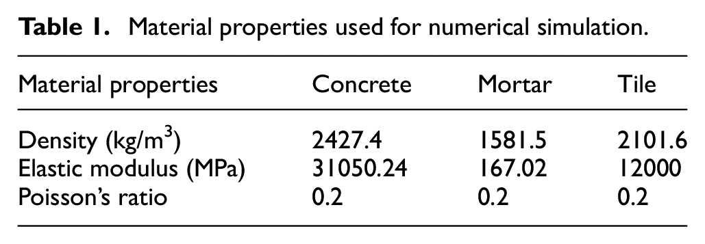
The hammer impact was simulated by applying a concentrated force at the tile centre, with its time history being the signal collected from an impact hammer in the laboratory testing. The tile-to-mortar and mortar-to-concrete interfaces were bonded, and the bottom face of the concrete base was set to be pinned. Linear hexahedral elements of type C3D8R were used for meshing, with a uniform mesh size of 1.5 mm for all three components. A time step of 2 ×10⁻⁶ was employed, which, along with the mesh size, was determined to be sufficient to capture the vibration responses while maintaining computational efficiency. The vibration responses were recorded with a sampling frequency of 520 kHz by collecting the time history of the in-plane displacements at the centres of the four quadrants (Q1–Q4 in Figure 1) on the tile surface. Such settings have been successfully verified to simulate the situations in experimental testing to be introduced in section ‘Experimental testing’. 34
A variety of defect scenarios were simulated using this model to generate a comprehensive database for network training. To create scenarios with random occurrences of debonding, two parameters were first defined: the defect diameter and centre position. The defect diameter (d) ranged from 10 to 40 mm in one-unit increments, and their centre positions were defined by x and y coordinates (Figure 4). To ensure the void does not exceed the boundaries of the 125 × 125 mm square, both x and y were constrained to the range of 20 to 105 mm. 300 Random combinations of x, y and d were generated using MATLAB, and the corresponding vibration responses were simulated by the numerical model.
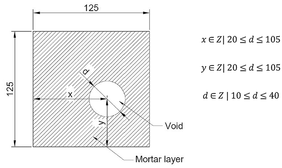
Void in the mortar layer with random position and random diameter (unit: mm).
Experimental testing
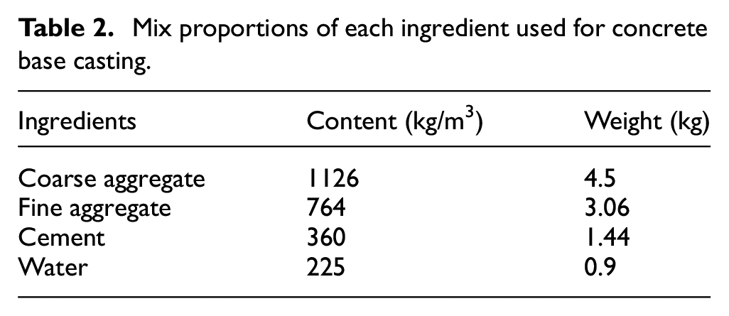
The concrete base was cast using the mix proportions outlined in Table 2. Following the demoulding of the base and a 28-days period of air curing, the mortar was trowelled onto it. The artificial debonding was introduced by inserting a 9 mm-thick PVC tube into the mortar layer during the trowelling process (Figure 5(a)). PVC tubes with inner diameters of 18, 20, 27, 30 and 34 mm were randomly inserted within the mortar layer on different panels. Together with the benchmark, the three classes, C1, C2 and C3, each have the same number of experimental damage scenarios. The ceramic tiles were subsequently affixed to the mortar, and after a drying period of 14 days, four lead zirconate titanate (PZT) sensors were attached to the centres of the four quadrants of the tile panel (Figure 5(b)). To stimulate the system, a Brüel & Kjær impact hammer of type 8206 was used to strike the tile. Signals from both the hammer and the PZTs were captured by a Tektronix® (Beaverton, OR, USA) MSO46 mixed signal oscilloscope, operating at a sampling rate of 6.25 million samples per second. It should be noted that this sampling rate was different from that of the simulation. However, the key frequency information from simulation and experiments would be consistent, as both sampling frequencies are significantly higher than the main frequency bands of interest, which are captured by CWT.
Mix proportions of each ingredient used for concrete base casting.
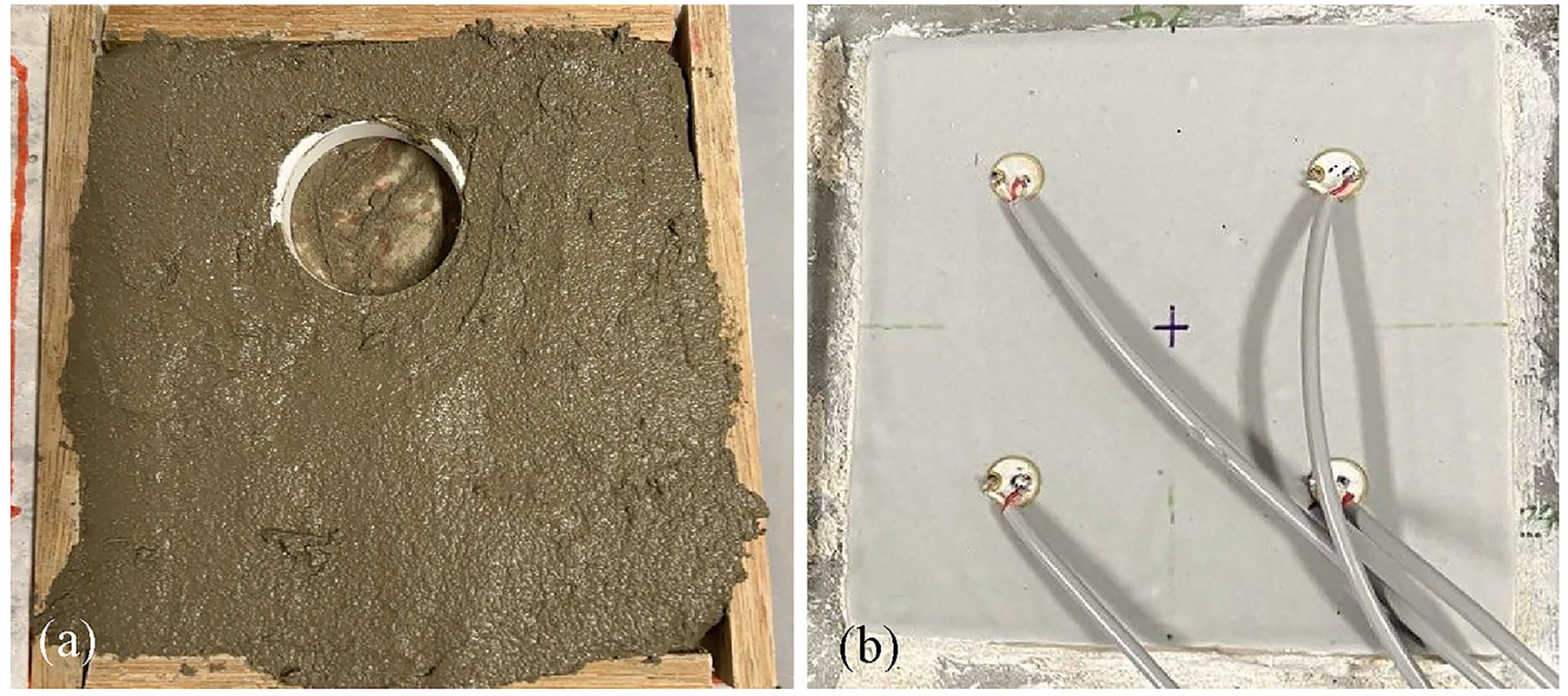
Artificial defect (a) and surface-bonded PZT sensors at four quadrants (b).
Signal-to-image transformation
The obtained data was transformed into scalograms using a CWT as 35 :
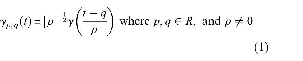
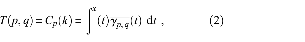
where
In this study, the analytic Morse (3,60) wavelet was used, where 3 is the symmetry and 60 is the time-bandwidth product. A time window capturing all relevant waveforms was selected to ensure that no critical information is omitted. The colour intensity of each point on the scalogram indicates the magnitude of the CWT coefficient at a specific time–frequency combination. By examining the scalograms, insights can be gained regarding the energy distribution across the frequency within the signal. Therefore, localised energy variations caused by different structural health conditions can be captured in these time–frequency images. 36
Figure 6 illustrates three sample scalograms of each class with the size of (440, 436, 3), computed from the simulated data using CWT in MATLAB. The dimension (440, 436, 3) represents the number of pixels in height, width and the number of colour channels respectively. Each scalogram seamlessly combines four smaller scalograms from the four quadrants of the tile panel. It can be seen that the scalograms of the three classes exhibit distinct patterns. C1, which corresponds to small debonding, displays a clear pattern with minimal variation in frequency content. C2 shows more complex features with greater dispersion in frequency, reflecting the presence of larger debonding compared to C1. C3, which corresponds to the most severe debonding, displays highly fragmented patterns, suggesting that the structural behaviour has been significantly altered. A total of 300 damage cases were simulated, with 105 belonging to the C1 class, 96 to the C2 class and 99 to the C3 class. The dataset was divided into training, validating and testing subsets, where training and validating datasets were augmented to enhance their diversity. The augmentation involves rearranging the positions of the four smaller scalograms within each individual scalogram. Mathematically, the number of permutations for n elements is given by:

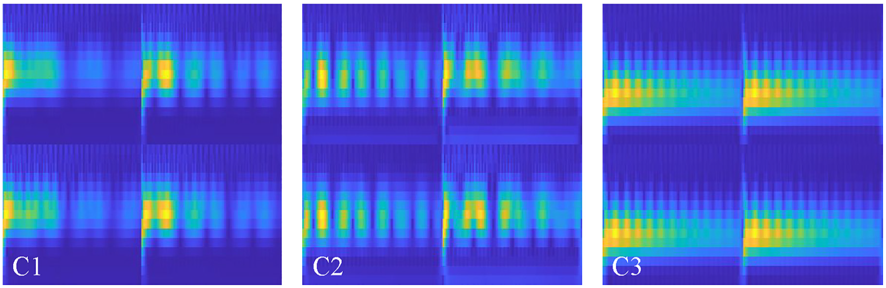
Sample scalograms from simulation of classes C1, C2 and C3.
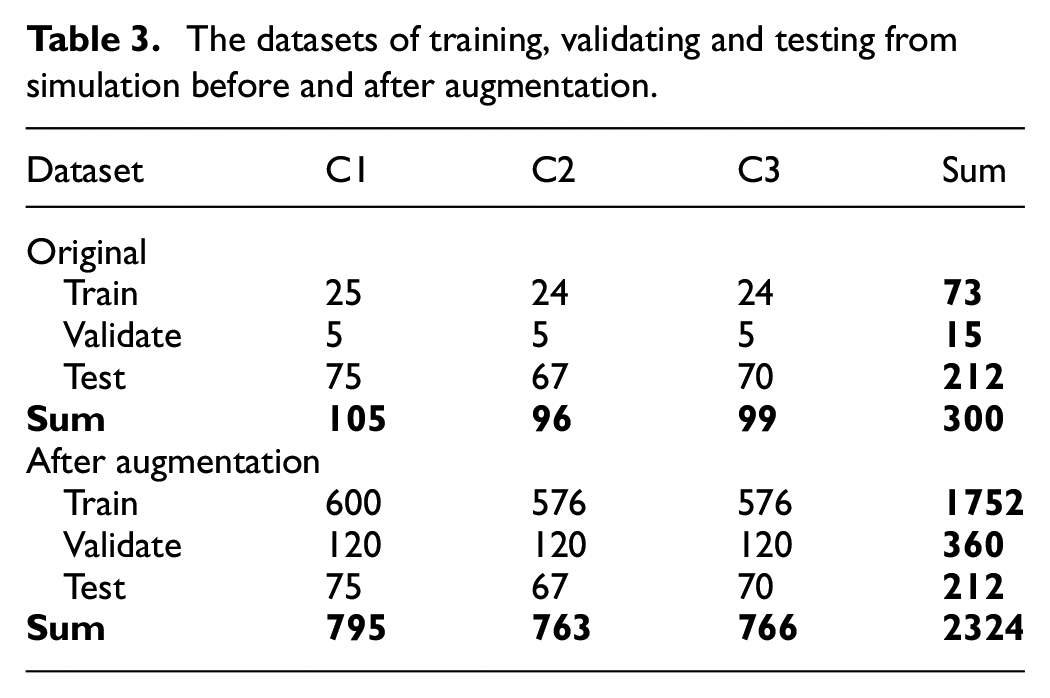
In this case with n corresponding to four smaller scalograms of the four quadrants, the total number of unique arrangements is 24. This was accomplished using a built-in permutation function in MATLAB, which systematically generated all 24 unique arrangements for each damage case (Figure 7). Since each damage case corresponds to the debonding of a specific size, this augmentation method generates additional cases with the same debonding size but with different spatial distributions. In this way, the dataset can be effectively augmented by a factor of 24, which improves the model’s ability to capture a wider range of patterns and features. The testing dataset remained unaugmented to mitigate the risk of overfitting. To maintain an 8:1:1 proportion, 73 cases were used for training (equivalent to 1752 cases after augmentation), 15 cases for validation (equivalent to 360 cases after augmentation) and 212 cases for testing. Table 3 summarises all these damage cases from the simulation before and after augmentation.
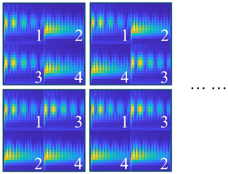
Permutations of four smaller scalograms for data augmentation.
The datasets of training, validating and testing from simulation before and after augmentation.
To facilitate the labelling process, these images were systematically organised into folders, whose names served as class labels. When the dataset was imported into the model, the framework automatically recognised the folder names as class labels, simplifying the data loading and labelling process.
Network training and results
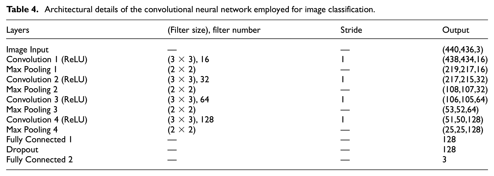
The simulated damage cases were first used to train and validate the designed CNN, with its architectural details illustrated in Table 4. It consists of four convolutional layers, each activated by the rectified linear unit (ReLU) function, and subsequently followed by max-pooling layers for downsampling as shown in Figure 2. In addition, there are two fully connected layers with SoftMax function that classify the data into three output classes.
Architectural details of the convolutional neural network employed for image classification.
The network training process was performed on a computer with an AMD Ryzen™ 7 5800X 8-Core Processor @3.80 GHz CPU, 32 GB installed memory (RAM) and a 6 GB GDDR6 memory NVIDIA GeForce GTX 1660 Ti graphics processing unit (GPU). The model was trained using a learning rate of 10−3, and the process was iterated for 50 epochs. The resulting training history is demonstrated in Figure 8, which shows the progression of model classification accuracy and loss function over successive training epochs, where both the accuracy and loss exhibit initial fluctuations but subsequently stabilise at the 50th epoch.
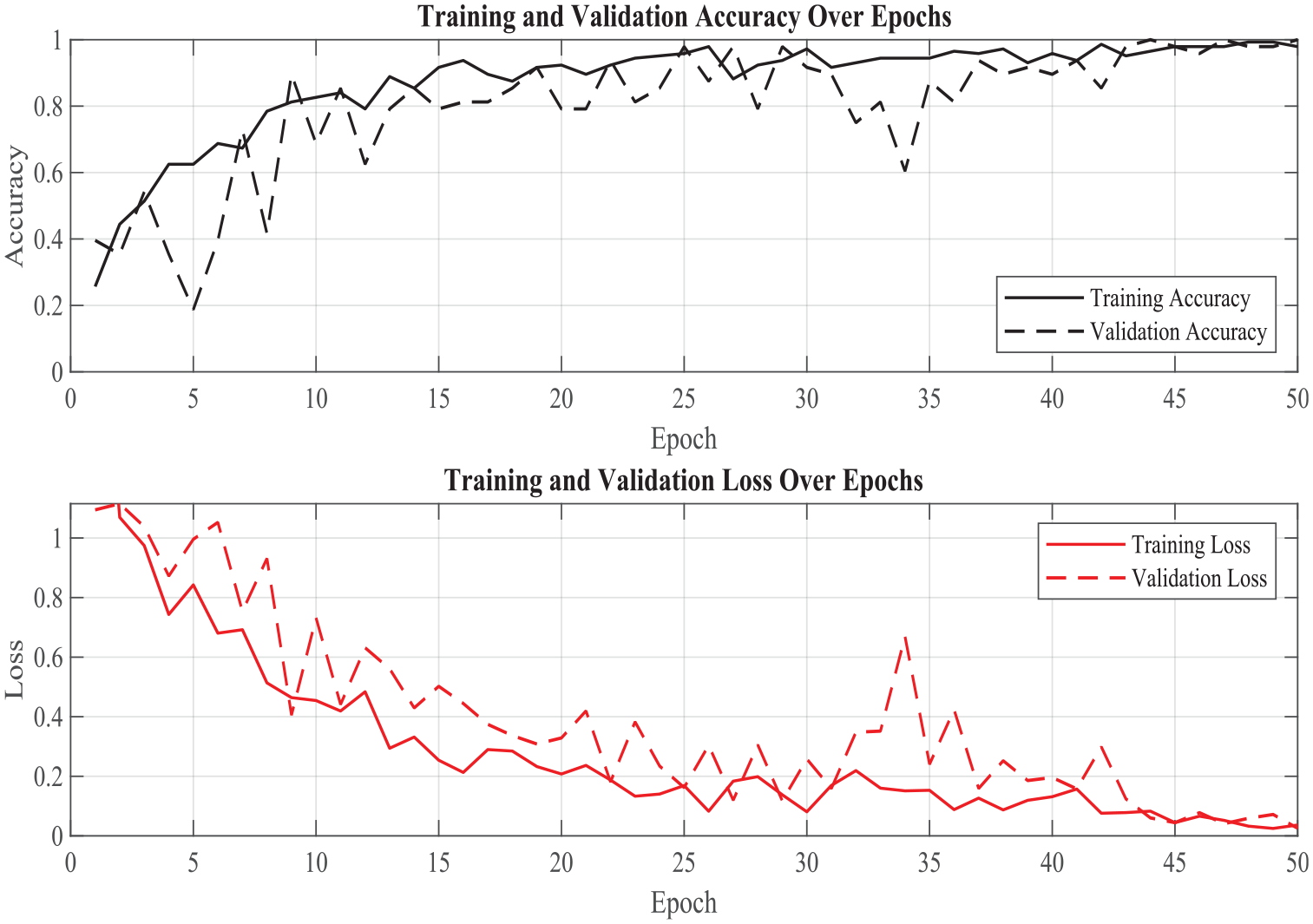
Training and validation accuracy and loss over epochs based on simulated data only.
The trained network was subsequently employed to make predictions on the testing dataset, and the resulting confusion matrix is presented in Figure 9. In this matrix, the diagonal elements represent the correctly classified instances for each class. Specifically, there were 71 true positives for C1, 59 for C2 and 70 for C3. Off-diagonal elements indicate misclassifications, with 4 instances from C1 incorrectly classified as C2, 8 instances from C2 misclassified as C1 and C3 and no instances from C3 misclassified. To better visualise the performance of the trained network in classifying the simulated data, a classification report was generated as shown in Table 5, where precision, recall, and F1-score, as frequently employed metrics in the statistical analysis of classification tasks, are listed to evaluate the accuracy of the classification outcomes. 37
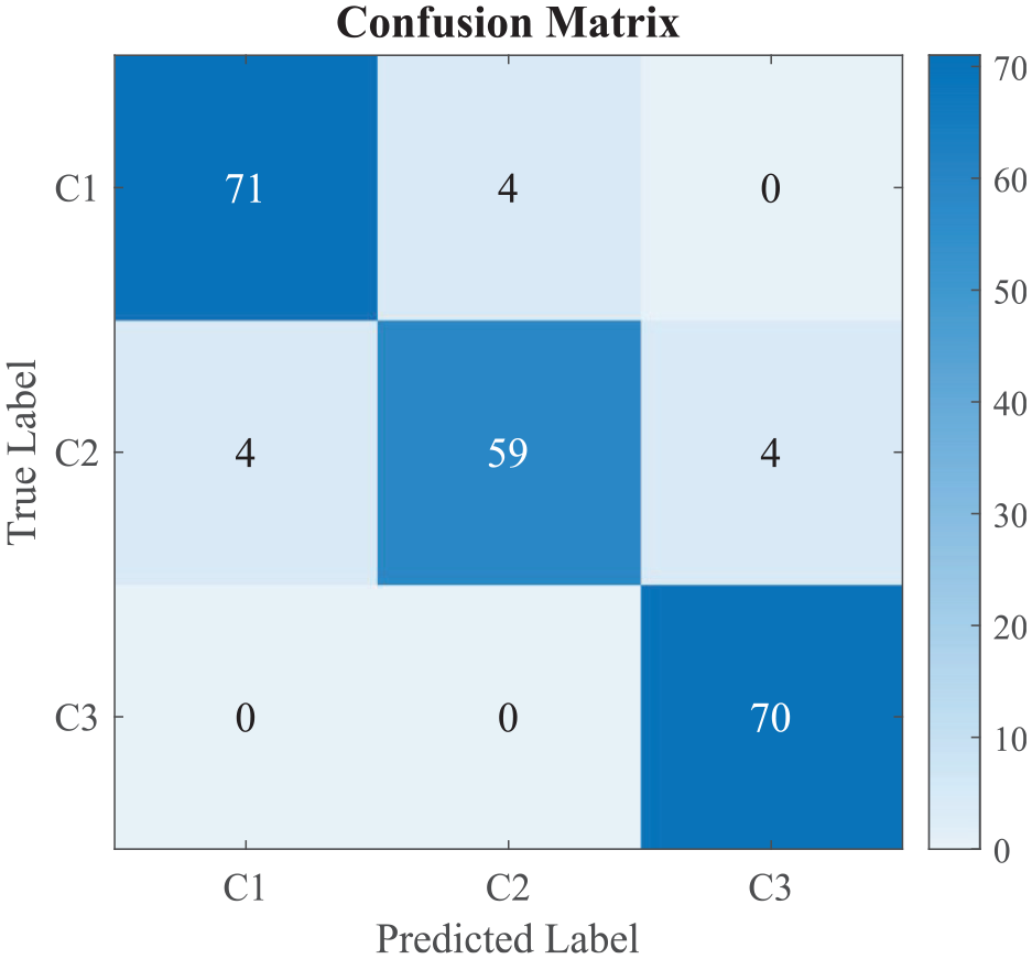
Confusion matrix of predicting simulated testing dataset using network trained by simulated data only.
Classification report of predicting simulated testing dataset based on the confusion matrix.
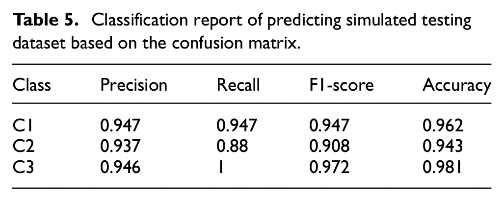
The results reveal a high accuracy for classes C1 and C3, but a relatively lower accuracy for class C2. This may be attributed to a relatively smaller volume of the training and validation dataset for class C2, potentially hindering the network’s ability to learn features as effectively as it does for the other two classes. In addition, it is worth noting that class C2 corresponds to damage cases within the 20–30 mm diameter range, which includes borderline data of 20 and 30 mm that could be potentially misclassified into classes C1 and C3 respectively. In contrast, the high accuracy of class C3 could be attributed to the large damage size that results in distinct responses from the other classes. In this case, the model can readily differentiate these data, leading to high-accuracy predictions. Overall, the trained model demonstrates good accuracy in predicting the testing dataset, which proves the effectiveness of the proposed methodology.
Experimental validation
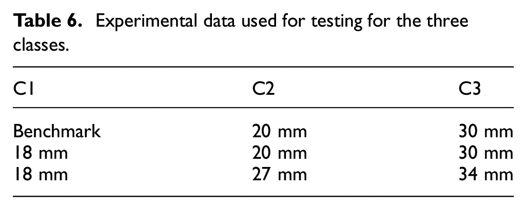
While the aforementioned results are derived from simulated data only, it is important to acknowledge that they hold limited practical significance if the model cannot effectively predict real-world data. Therefore, to improve the practical feasibility of the proposed methodology, experimental data collected from the laboratory specimens were employed as the testing dataset to evaluate the trained network. Table 6 shows the experimental specimens used for this purpose for the three classes respectively.
Experimental data used for testing for the three classes.
The sample scalograms of each class are shown in Figure 10. Similar to the simulated scalograms (Figure 6), the experimental scalograms show clear distinctions between classes, displaying more complex and dispersed patterns as the debonding size increases. However, C3 differs significantly from that of the simulated results. This can be attributed to the inevitable differences between the numerical model and the laboratory specimen, as reflected in the differences between the simulated and experimental scalograms shown in Figures 6 and 10, particularly in the C3 class. In detail, although the material properties were measured and input into the numerical model, actual properties may vary due to manufacturing inconsistencies or measurement errors. Real materials often exhibit anisotropic behaviour, whereas the simulation always assumes homogeneity. Additionally, the actual boundary conditions might be more complicated than those simulated in the numerical model. During the specimen preparation, the sizes and positions of the concrete, mortar layers and tiles may not be as precise as in the simulation. The individual differences of PZT sensors and the effect of background noises during signal collection in experiments are also unavoidable.
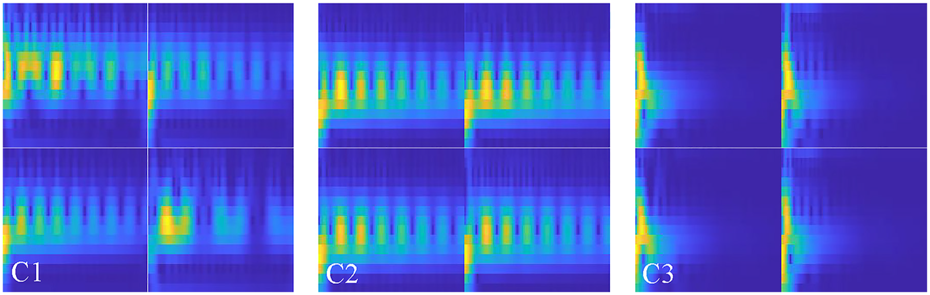
Sample scalograms from experiments of classes C1, C2 and C3.
Another notable difference is that the simulated waveform exhibited a longer duration compared to the experimental one, which may be attributed to differences in damping characteristics between the simulated and real-world conditions. Using the same time window for both simulated and experimental scalograms may cover the genuine signal features occurring at the early stage of vibration responses. Therefore, the time window for the experimental scalograms was specifically set to just include all collected waveforms to ensure comparability with the simulated scalograms, while the frequency bandwidth remains the same as that of the simulated scalograms.
Figure 11 illustrates the prediction results on the experimental data using the network trained solely on simulated data. It is evident that the network exhibits lower accuracy compared to Figure 9, with a majority of cases being classified into C3. The network trained by simulated data only would struggle to adapt to the complexities and variations present in real experimental data, despite that different time windows for the simulated and experimental scalograms have been applied to alleviate these differences. To generalise and improve the model’s ability to real-world scenarios, experimental data was then incorporated into the training and validation process in this study. This provides the model with a broader dataset that enhances its capacity to achieve accurate predictions on real-world data.
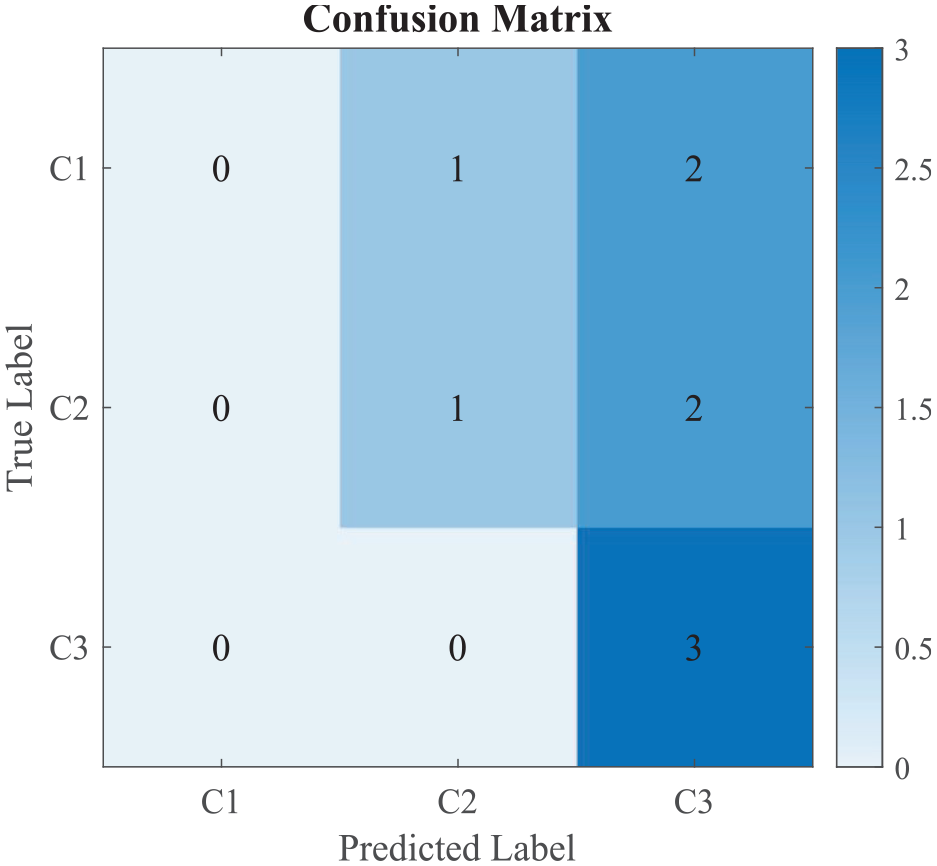
Confusion matrix of predicting experimental testing dataset using network trained by simulated data only.
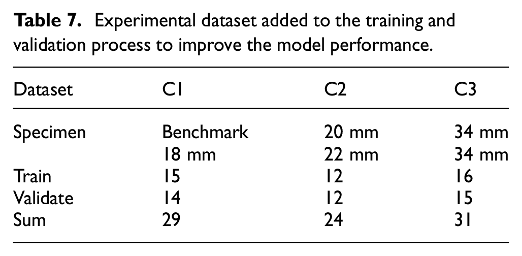
Table 7 shows the specimens prepared and the quantity of experimental data integrated into the training and validation process for the three classes respectively. As a means of data augmentation, vibration responses for each specimen were collected multiple times by varying the hammer hit forces. This method was distinct and independent from that applied to the simulated data. It was designed to introduce variability that reflects real-world conditions, where tap testing inspectors apply varying impact forces to the targets. It is noteworthy that these data originated from other specimens than those where the data were employed for testing (Table 6), ensuring a comprehensive and independent evaluation of the model performance. The trained network would then be used to predict the same experimental testing dataset (Table 6) to guarantee a fair comparison between the simulated-only and simulated-experimented (hybrid) networks.
Experimental dataset added to the training and validation process to improve the model performance.
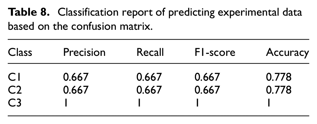
A smaller learning rate of 5 × 10⁻⁴ and 100 epochs were used to allow for gradual and precise parameter adjustments, which is crucial for handling the increased complexity and noise in the experimental data. The training history and the corresponding prediction confusion matrix are presented in Figures 12 and 13 respectively. Compared to the simulated-only network, the hybrid network demonstrates better accuracy in predicting the experimental data, which verifies the beneficial impact of incorporating experimental data into the training process. However, in both C1 and C2 classes, one instance was still misclassified. To be specific, an 18 mm damage case was incorrectly classified as C2, and a 20 mm damage case was misclassified as C1. Given that these two damage sizes are quite comparable, their responses may be quite similar to those of the adjacent classes. This can lead to challenges for the network to accurately distinguish these cases. Consequently, as listed in Table 8, classes C1 and C2 exhibit lower prediction accuracies compared to class C3, similar to the simulated-only scenario.
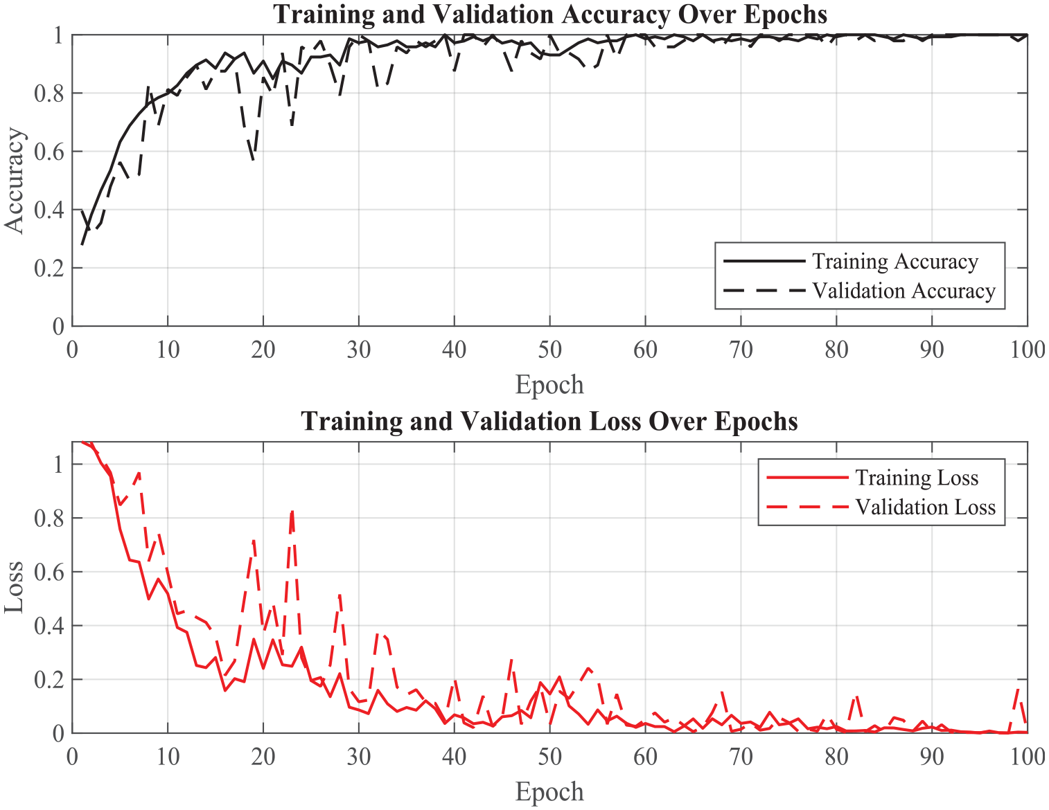
Training and validation accuracy and loss over epochs based on both simulated and experimental data.
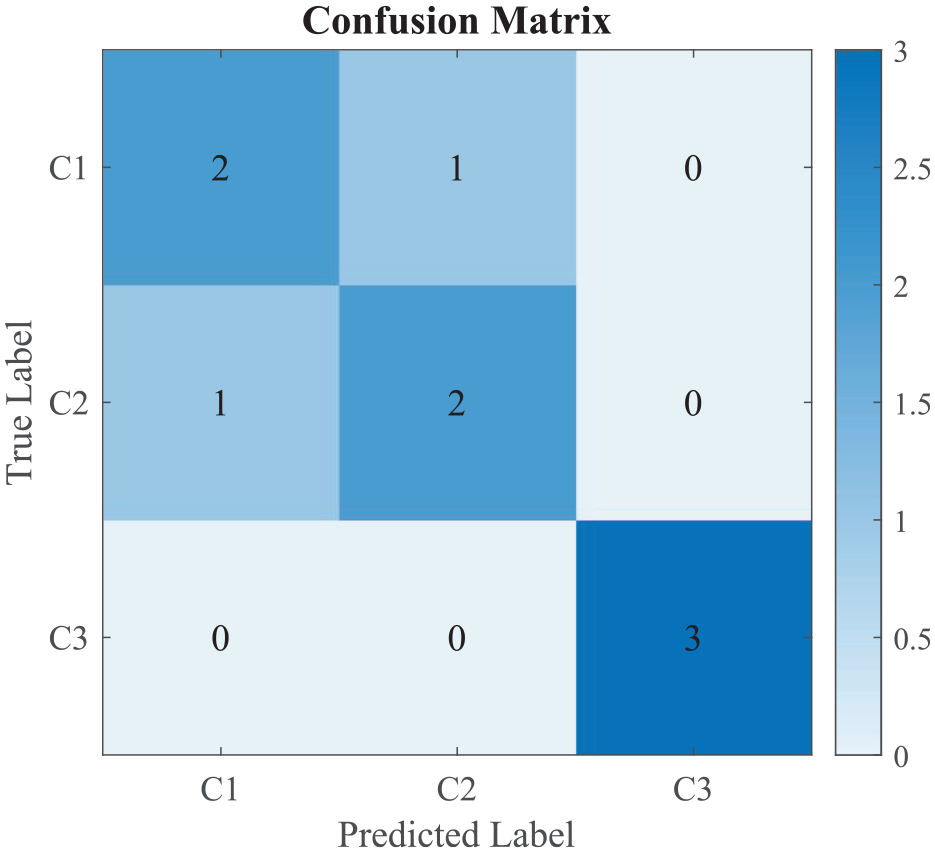
Confusion matrix of predicting experimental testing dataset using the network trained by both simulated and experimental data.
Classification report of predicting experimental data based on the confusion matrix.
Despite the fact that the accuracy in predicting the experimental data did not reach the same level as predicting the simulated data, the hybrid network yielded a higher accuracy when comparing Figures 11 and 13 for potential real-world applications. It is worth noting that the availability of experimental specimens is constrained due to the labour-intensive nature of specimen preparation, resulting in a limited experimental testing dataset that is equivalent to only 4.8% of the simulated testing dataset. This size disparity consequently contributes to a relatively lower accuracy observed in the prediction. In summary, the network has demonstrated good performance in classifying damage cases into their respective size categories but experienced challenges for borderline sizes. To enhance this aspect in the future, further refinement of the class structure may be considered with more experimental data involved.
Conclusion
This study presents a methodology for automated classification of interfacial debonding sizes in ACTs based on vibration responses. Damage scenarios featuring random debonding positions and sizes were generated through numerical simulation and experimental testing. The in-plane displacements at the four quadrants of the tile surface were collected during the hammer impact as the vibration responses. The waveform data from four quadrants of the tile was subsequently transformed into scalograms using CWT, which were then seamlessly combined to form a single scalogram representing a damage case. For training and validation datasets, data augmentation was implemented by repositioning the scalograms of the four quadrants for each damage case.
Initially, the CNN was trained using simulated data only, achieving high accuracy in predicting simulated data that were not involved in training and validation. To broaden its real-world application, experimental data was subsequently integrated into the training and validation processes. While the hybrid-trained network demonstrated good performance in categorising the damage cases, it encountered difficulties in classifying cases with sizes at the boundary of two adjacent classes. The restricted volume of the experimental dataset might have imposed limitations on the performance of the trained network.
The current experimental setup, while effective in a controlled environment, may not fully replicate the complexities of real-world applications. Nonetheless, the feasibility of the proposed technique has been proven as a foundational framework for evaluating the severity of interfacial debonding in ACTs. This study investigates circular debonding as a foundational case, but the proposed method is adaptable for more complex real-world patterns exhibiting equivalent vibration characteristics. Future work will incorporate a larger experimental dataset to further refine the approach and enhance its applicability to real-world scenarios. On the other hand, the class structure will be refined to improve the prediction accuracy on borderline cases.
Footnotes
Declaration of conflicting interests
The author(s) declared no potential conflicts of interest with respect to the research, authorship and/or publication of this article.
Funding
The author(s) disclosed receipt of the following financial support for the research, authorship and/or publication of this article: The authors are grateful for the financial support of the Australian Research Council (DP200102497).