
Abstract
In structural health monitoring using computer vision, deep learning-based damage identification and three-dimensional (3D) reconstruction of the structure are current hot topics. Traditional photogrammetry techniques are cost-inefficient and time-consuming for 3D reconstruction, and there is no such solid 3D pixelwise damage mapping technique. To overcome these limitations, a new deep neural network (DNN)-based 3D reconstruction method, including damage mapping, is proposed in this article. As the DNN-based 3D reconstruction method, Nerfacto—an advanced version of Neural Radiance Fields models—was selected for achieving high-fidelity 3D reconstruction. This Nerfacto model was modified to create a high-definition 3D reconstruction model of the structure of interest (i.e., a 3-span bridge system). To map damages within the reconstructed 3D model using the modified Nerfacto, the state-of-the-art semantic transformer representation network (STRNet) with test time augmentation (TTA) was also developed for precise pixel-wise crack segmentation. Through extensive case studies, including parametric studies, we found that the modified Nerfacto can learn various appearance features of the structure and generate a very high-definition 3D model. Moreover, the segmented damage (i.e., cracks) from the STRNet with TTA could be mapped onto the reconstructed 3D model. This study demonstrates the potential of combining deep learning with 3D reconstruction for proactive and preventative maintenance strategies, ensuring the safety and longevity of vital structural assets.
Keywords
Introduction
Structural health monitoring (SHM) is a critical process for assessing the condition and predicting the lifespan of infrastructural assets. 1 It plays a vital role in ensuring the safety and longevity of structures while aiding in cost-effective maintenance. The importance of SHM worldwide is highlighted by the continuous aging of bridge infrastructure. For example, in Canada, since the 1970s, there has been a noticeable increase in the average age of bridges, indicating a consistent aging process exacerbated by inadequate investment. 2 By 2003, many federal and provincial bridges had surpassed half of their expected 46-year lifespan. Federal bridges, though only 3% of the total, averaged 26.4 years old, while provincial bridges, which make up 57% of the total, saw their average age rise from 15.4 to 24.6 years from 1963 to 2003, largely due to low provincial investment. Municipal bridges, younger on average at 19.0 years, comprised 39% of the infrastructure. 3 This aging trend, especially among provincial bridges, shows the need for regular inspections to maintain safety and prolong their usable life. Regularly conducted SHM not only ensures structural safety but also contributes to reducing maintenance costs, making it an indispensable practice in the field of civil engineering and infrastructure management. 4
While SHM systems have traditionally relied on vibration sensors, 5 these methods face challenges, particularly when applied to large-scale civil infrastructures. Techniques that utilize numerical methods, as explored in various studies, often struggle with the effects of uncertainty and non-uniform environmental influences. 6 A major hurdle in these approaches is the difficulty in distinguishing between actual structural damage, malfunctions in the sensory system, and noisy signals. This complexity necessitates on-site verification of the sensing systems and the structures themselves, which requires qualified technicians to visit the structure, resulting in an unnecessary use of time and financial resources.
Among various indicators of structural deficiencies, cracks are particularly noteworthy. Commonly arising from factors such as cyclical loading, drying shrinkage, thermal contraction and expansion, and overall structural deterioration, cracks are critical markers that demand attention. 7 Addressing these damages promptly is essential for ensuring the long-term durability of structures and preventing the propagation of cracking. Effective monitoring and sealing of cracks are therefore pivotal in maintaining structural integrity and extending the lifespan of infrastructural assets. 8
The evolution of vision-based equipment and image-processing technologies has advanced the field of SHM. Computer vision has emerged as an efficient tool for damage identification, offering a more reliable alternative to the traditional visual evaluations conducted by human experts, which are often labor-intensive and subject to variability.9,10
Traditional image-based techniques for crack segmentation, detection, and classification have been extensively researched. 11 These methods, including thresholding-based, edge-based, and data-driven approaches, have gradually become less favored due to limitations in accuracy and difficulties in crack segmentation in complex backgrounds. 12 In contrast, the advent of deep learning, particularly deep convolutional neural networks (CNNs), has revolutionized damage detection. Deep CNNs excel in extracting multilevel robust features from images and continuously refining internal parameters for automatic recognition.13–15
A notable development in this domain is the U-net architecture, initially proposed for medical image analysis, 16 which has been effectively adapted for both medical and non-medical image segmentation, including crack detection.17,18 Further advancements have been made; Fu et al. 19 also attempted to integrate Deeplabv3+ and Xception for bridge crack segmentation. Despite these developments, challenges remain, particularly in applying U-net to complex scenes with diverse visual elements. Addressing this, an object-specific network targeting structural cracks, namely SDDNet, 20 was developed using various advanced modules (DenSep module and Atrous Spatial Pyramid Pooling (ASPP)) with advanced operations such as depthwise convolution and dilated convolutions. Another object-specific network, semantic transformer representation network (STRNet), 21 was proposed by designing an STR module that has three different configurations that are regularly repeated with different filters and activation functions, including attention modules in the encoder and decoder for crack segmentation. This offers real-time processing of normal video with a large input frame size of 1200 × 800 × 3, achieving state-of-the-art (SOTA) performance with a mean intersection over union (mIoU) of 0.93 in varied and complex scene environments. These advances in computer vision and deep learning emphasize the dynamic nature of SHM and underscore the shift from traditional methods to more sophisticated and automated techniques that increase the accuracy and efficiency of structural damage detection.
A critical challenge in applying CNNs to damage detection in real structures is the requirement for extensive training samples. 22 Capturing a comprehensive range of damage scenarios for in-service structures to train these models is often difficult, if not impossible. This limitation can restrict the practical application of CNNs in real-world SHM. 23 To address this issue, researchers have explored methods like transfer learning and semi-supervised learning. Transfer learning, as discussed by Teng et al., 24 involves adapting a pre-trained model to a new but related problem, while semi-supervised learning, as described by Xiang et al., 25 leverages a combination of labeled and unlabeled data for training. However, both approaches require re-training, which can be time-consuming and resource-intensive. Additionally, they often necessitate larger datasets.
In the context of SHM, where time efficiency is paramount for rapid monitoring and assessment, 26 test time augmentation (TTA) emerges as a valuable method. TTA involves applying various augmentations to the test images and then averaging or combining the predictions to improve the model’s performance. 27 This technique does not require retraining the model; instead, it enhances the prediction accuracy at the time of testing by leveraging diverse variations of the input data. As highlighted by Wang et al., 28 TTA operates similarly to an ensemble approach, combining results from different augmentations to achieve a more robust and accurate outcome. This makes TTA particularly suited for SHM applications where quick and reliable damage assessment is crucial.
The detection of damage in a single image in SHM, while useful, has limitations, especially when dealing with large structures. A single image typically covers only a small portion of an entire structure, making it challenging to contextualize the extent of the damage 29 and to localize the damage even though some articles have used geo-tagging for 2D damage localization.15,30,31 Therefore, accurately mapping detected damages from 2D images to 3D world coordinates is crucial, particularly for large structures like bridges. This process enables a more comprehensive understanding of the damage distribution and severity.
Recently, 3D reconstruction as a digital twin of structures has emerged as a transformative solution for intelligent SHM. It not only enhances the accuracy of damage assessment but also paves the way for more intelligent and predictive maintenance strategies.32,33 The 3D models generated for SHM purposes should contain enriched surface texture with high spatial resolution for damage assessment. 34 This involves creating a 3D representation of an object, where data points can be acquired through photogrammetric methods or laser scanning. In computer vision, various techniques are implemented using multiple images, as opposed to relying solely on stereo images. 35 One such technique is Structure from Motion (SfM), which has been effectively used to create detailed 3D models of objects and landscapes.35,36 For instance, Xue et al. 37 utilized an SfM-based deep learning method to assess defects in tunnels, demonstrating the method’s applicability in monitoring expansive areas.
Photogrammetry has also been utilized to project detected concrete cracks onto reconstructed 3D models, with CNN-based methods like UNet enhancing the accuracy of these projections. 38 However, photogrammetry-based 3D reconstruction presents its challenges. It can be time-consuming and computationally intensive. 39 Moreover, reconstructing planar surfaces solely through photogrammetry poses specific difficulties, so lasers can be used to overcome these, 40 necessitating the exploration of more efficient and effective methods in SHM.
In the realm of recent 3D reconstruction, neural radiance fields (NeRF), introduced by Mildenhall et al., 41 have emerged as a breakthrough approach, attracting researchers' attention as a viable alternative to traditional photogrammetry. This method distinguishes itself from photogrammetry by effectively scanning objects with sparse feature points, thus offering a more flexible solution for 3D reconstruction. Departing from the reliance on manual texture mapping and geometric primitives such as triangles and voxels, characteristic of traditional methods, NeRF employs a neural network to directly model the visual characteristics of a scene. It learns the scenes from images collected from different camera locations. This novel approach facilitates capturing complex lighting effects, including reflections and transparencies, by creating unique representations of points from varying viewing angles. As a result, NeRF achieves a more detailed and accurate rendering of scenes, 42 presenting a potential method for use in SHM.
Recent research has highlighted the potential of utilizing NeRF for advanced applications in structural health monitoring and construction automation. Pal et al. 43 integrated NeRF with building information modeling (BIM) systems to visually monitor the progress of construction activities, demonstrating NeRF’s ability to support project management by providing precise visual documentation of construction stages. Additionally, Yu et al. 44 applied NeRF to 3D damage mapping on underwater bridge piers, showcasing its effectiveness in capturing detailed representations of structural damages. However, these applications typically focus on specific parts or limited areas, showing particular viewpoints or sections of structures.
This limited scope is partly due to NeRF’s inherent limitations in generating 3D reconstructed models: (1) it requires significant computational resources, therefore it only works for very small-sized objects such as chairs or desks; (2) it has limited performance in predicting the actual pixel opacity and RGB values due to poor generalization performance; and (3) it is very sensitive to hyperparameters, making it unreliable for large-scale civil infrastructures.
To address the limitations of the original NeRF, particularly in large-scale environments, Tancik et al. 45 introduced the prototype Nerfacto model, an advanced variant designed to enhance 3D scene reconstruction capabilities. This model tackles computational challenges by employing a smaller neural network architecture in conjunction with multiresolution hash encoding and proposal sampling techniques, thereby reducing computational demands. Additionally, the Nerfacto model enhances the accuracy of RGB value predictions through advanced methods such as proposal sampling, appearance embedding, and spherical harmonics encoding. However, we find that this prototype Nerfacto still faces limitations when applied to civil infrastructure. 46
To overcome these challenges, this article proposes an enhanced approach to Nerfacto-based 3D damage mapping for structures. The proposed method incorporates advanced deep learning-based pixelwise crack segmentation using state-of-the-art (SOTA) models, STRNet and TTA. This article is composed of section “Methodology,” section “Case studies,” section “Conclusions,” and section “References.”
Methodology
In this article, we propose a new 3D damage mapping method by integrating an advanced deep learning-based pixelwise damage segmentation method with a 3D image reconstruction method. The overall process of the proposed method is illustrated in Figure 1. As the initial step, 2D RGB images of a structure of interest are collected. For 3D reconstruction of the structure, SfM is used to extract camera parameters using the Agisoft Metashape software tool. 47 The calculated camera parameters are then forwarded to the Nerfacto model, 45 which is an advanced NeRF-based model. Additionally, the collected 2D RGB images are fed into the newly proposed TTA-STRNet for pixelwise damage segmentation. The 2D images with segmented damage are subsequently input into the Nerfacto model for 3D rendering and 3D damage mapping using the calculated camera parameters. Ultimately, the reconstructed 3D damage map can be displayed using any 3D visualization tool as comprehensive damage information. All the details of each step are described in the following subsections.
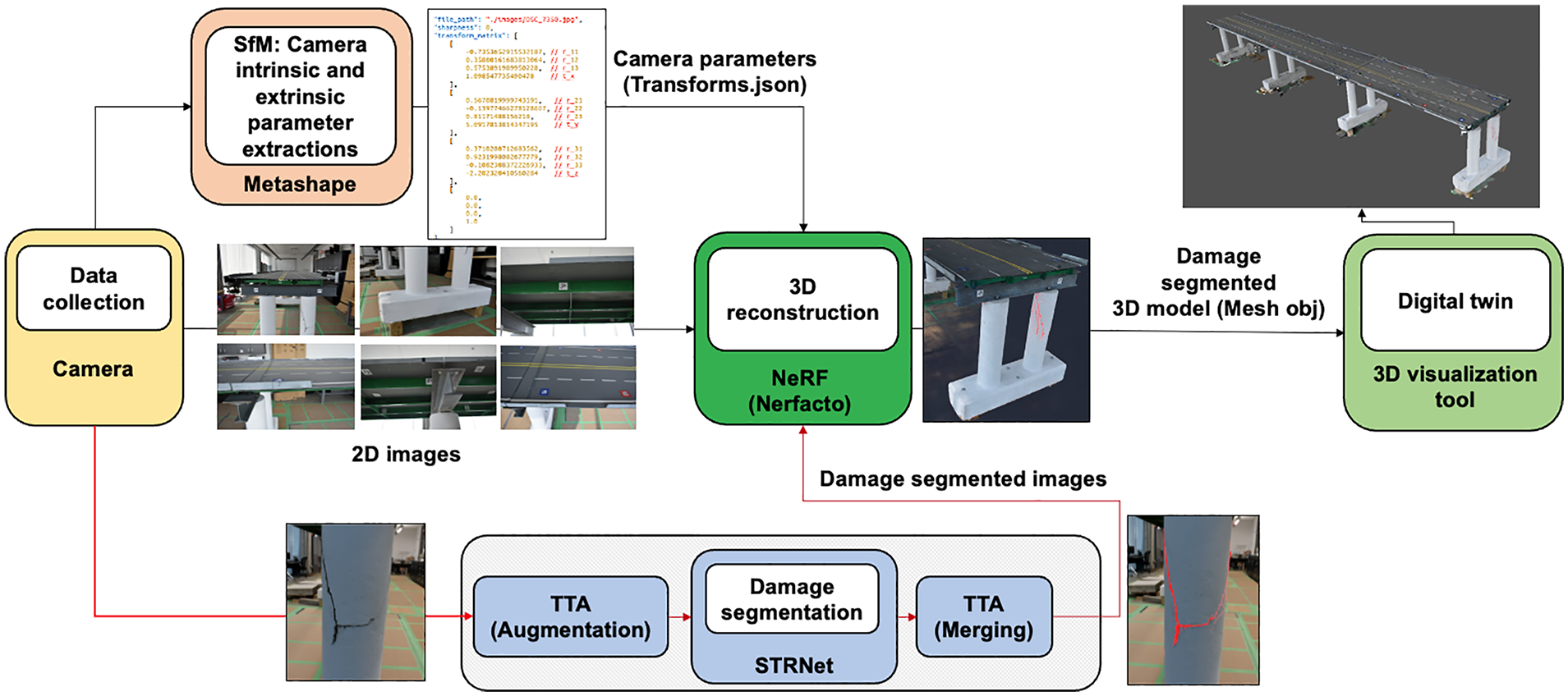
Flowchart of the proposed method framework.
Camera parameter extraction
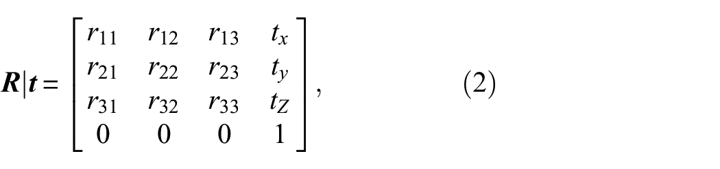
To employ the NeRF-based Nerfacto model in our methodology for 3D reconstruction, with segmented damage or without segmented damage, it is essential to obtain each image’s intrinsic and extrinsic camera parameters, represented by the matrices
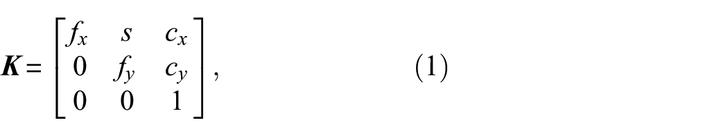
where
where
These parameters (
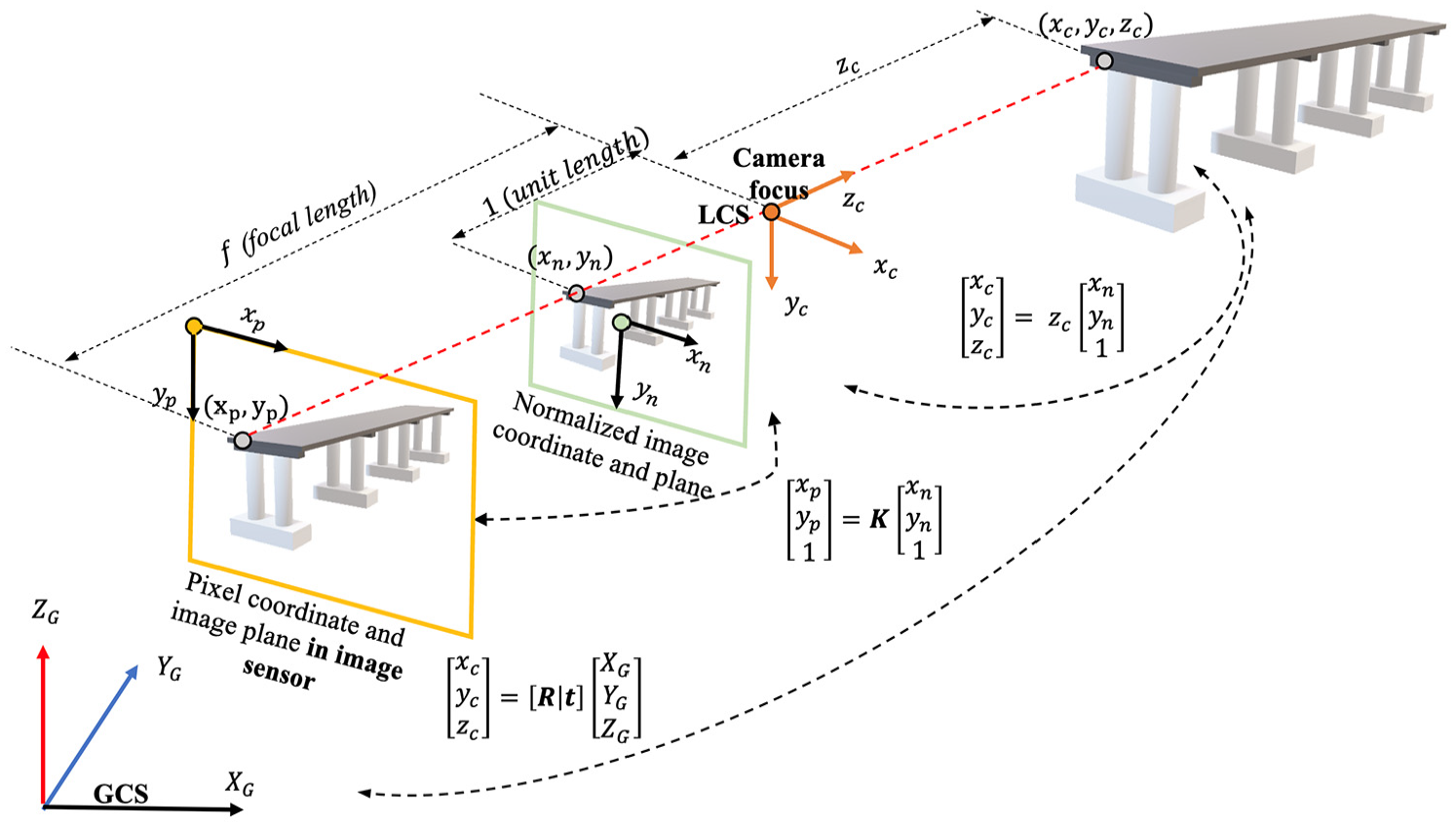
Camera projection model.
As shown in Figure 2, when an arbitrary 3D point
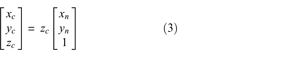
These normalized image coordinates
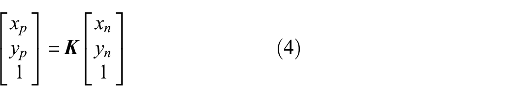
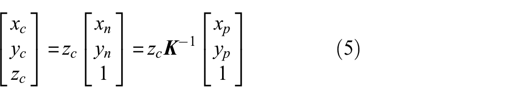
Consequently, Equation (5) explains how the 3D spatial coordinates
When images of an object are captured from varying angles and positions, the LCS for each image differs. By applying the extrinsic matrix
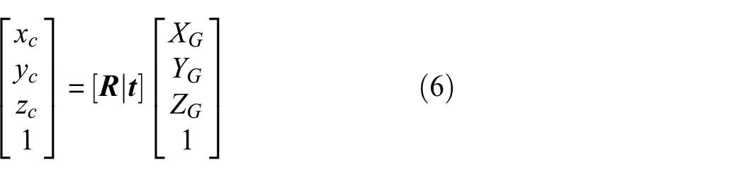
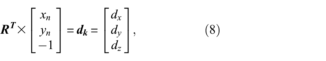
The first 3

where each
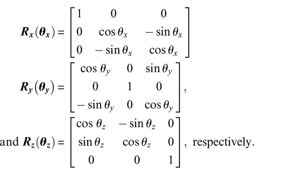
To obtain the extrinsic camera matrix
TTA-STRNet crack segmentation
In this article, the main contribution is the development of 3D damage mapping, therefore, for the crack damage segmentation method, we utilized STRNet 21 for segmenting structural damage within 2D RGB images. STRNet, a sophisticated deep learning network, is tailored for real-time, pixel-level crack segmentation against complex backgrounds with large input image frames (1280 × 720). STRNet achieved a mIoU of 92.6% and a processing speed of 49 frames per second for the same image size, making it a state-of-the-art method in this field.
However, in this article, we use a specific bridge system that is in the lab, therefore, it is quite challenging to have various different testing images for the STRNet. To overcome this challenge, we combined TTA with STRNet as a solution. TTA is an image augmentation technique that can be used in the cases where there is only a limited number of testing images. This method can augment the limited testing images for the STRNet.
Test time augmentation
TTA is a methodology implemented during the testing phase, unlike standard data augmentation, which is applied during the training phase. TTA involves applying a series of image transformations, such as resizing, flipping, and rotating, during inference, and then aggregating the results to form a final prediction.
In our approach, as illustrated in Figure 3, images captured at a resolution of 2992 × 2000 pixels are used for 3D image reconstruction to achieve high-resolution results. However, for damage segmentation, the images are resized to 1280 × 720 and 2048 × 1024 because STRNet was originally developed as a real-time method for processing standard video frames with a size of 1280 × 720. After detecting damage, the images are rescaled back to their original dimensions (2992 × 2000), as shown in Figure 3. To further augment our data and enhance the model’s robustness, we apply horizontal and vertical flips as well as rotations (90°, 180°, and 270°). This augmentation strategy results in 12 distinct test cases, allowing us to evaluate the model's performance across various image sizes and material characteristics.
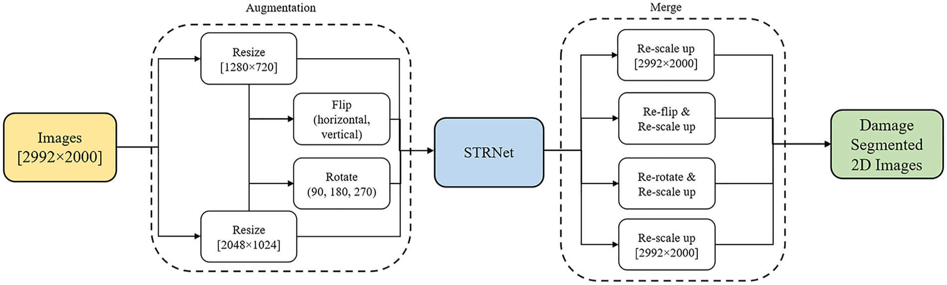
STRNet + TTA structure.
Integrating TTA with STRNet not only enhances the model’s performance without requiring retraining but also minimizes bias by analyzing multiple augmented versions of the same image during inference. This method improves the deep learning model’s accuracy and generalizability. By implementing various augmentations at test time and combining the outcomes, TTA functions in a manner akin to an ensemble method, ensuring prompt and accurate damage assessment essential for effective SHM. 28 The details of STRNet and TTA are elaborated upon in subsequent sections.
The semantic transformer representation network
The architecture of STRNet is specifically designed for crack segmentation, featuring an attention-based encoder and a multi-head attention-based decoder incorporated within the STR module, which is configured in three different ways and repeated irregularly 11 times. The inclusion of coarse up-sampling, a focal-Tversky loss function, and a learnable swish activation function simplifies the network's design without compromising its rapid processing capabilities. Figure 4 depicts the complete STRNet architecture, starting with the input images being processed initially in the first convolution block.
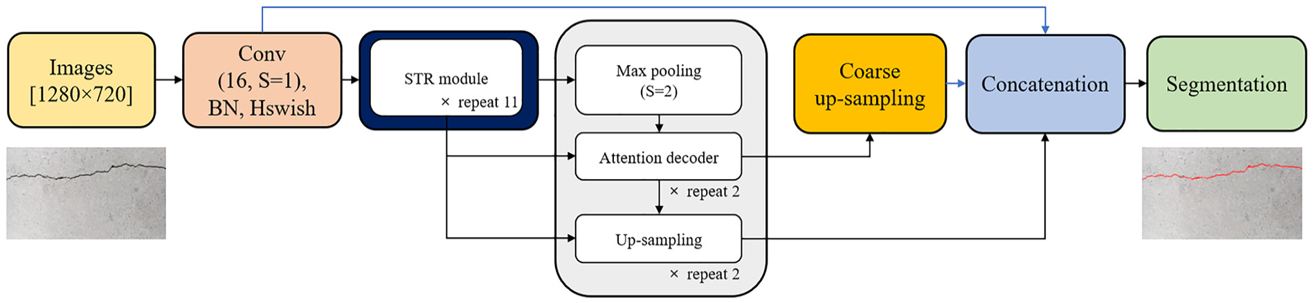
The STRNet architecture. 21
This block integrates convolution with the Hswish activation function 48 and batch normalization (BN). 49 The feature map produced by this convolutional block is then fed into the STR module, a process that repeats 11 times. After passing through the STR module, the output undergoes max pooling and is then input into the attention decoder. Utilizing skipped connections to retain multi-dimensional features, this decoder processes the data in two iterations. It then performs two types of up-sampling, utilizing both standard and coarse up-sampling techniques to return the data to the input image’s original dimensions. The standard up-sampling step is repeated twice, reactivating the skipped connections.
In the final step, the outputs from the up-sampling block, the initial convolution block, and the coarse up-sampling block are combined. This combined output is then subjected to pointwise convolution (PW). This convolution step yields the final output, enabling precise pixel-level segmentation of cracks. More details can be found in Kang and Cha. 21
NeRF for 3D reconstruction
The motivation for employing 3D reconstruction in our research stems from its capability to provide more intuitive visualizations, precise localization, and quantification of damage compared to traditional 2D methods. Additionally, 3D reconstructions can be exported as mesh OBJ files, which are beneficial for various downstream applications within the digital twin framework, such as 3D simulation and finite element analysis (FEA).
The original NeRF model, developed by Mildenhall et al., 41 synthesizes 3D models from 2D images by creating a scene with continuous volumetric functions encoded into a deep neural network. This network is comprised of a deep neural network (DNN) with fully connected layers. In the NeRF model, each point in space is assigned a density value that indicates its level of transparency or opacity and includes a view-dependent color that changes based on the viewing angle and distance. This deep neural network learns the RGB values and opacity of each pixel from the collected 2D image data through the training process. As a result, a well-trained NeRF model can generate highly detailed and photorealistic renderings from new viewpoints.
However, the original NeRF model exhibits certain limitations in terms of computational efficiency, memory usage, training speed, and rendering quality under different lighting conditions. To address these limitations, NeRF technology has evolved to include several specialized models, each designed to tackle specific challenges and enhance aspects of 3D reconstruction. For example, Mip-NeRF 360 50 utilized a proposal sampling method that iteratively refines 3D sample points to focus on areas with higher scene content, improving sampling efficiency. Instant-NGP 51 enhances training speed and computational efficiency through hash multi-resolution encoding. Another model, Ref-NeRF, 52 employs spherical harmonic encoding to efficiently capture directional information and realistically render complex lighting environments. Moreover, NeRF-W 53 introduces appearance embeddings to handle variations in training data conditions, such as different lighting setups. In this paper, we adopt the Nerfacto model, 45 which combines elements of Instant-NGP, Ref-NeRF, and NeRF-W. This integration enables the Nerfacto model to strike a balance between rapid training times and high-quality outputs.
Subsequent subsections will delve into the structure of the original NeRF model and the Nerfacto model in more detail, discussing how the coordinates of 3D points and the directions of rays for each image are determined using the camera intrinsic and extrinsic parameters discussed in section “Camera parameter extraction.”
Neural radiance fields
As mentioned earlier, the original NeRF model has considerable limitations. Therefore, in this paper, we implemented the enhanced Nerfacto model. The overall process of Nerfacto is quite similar to that of NeRF. Therefore, we will first explain the general workflow of the NeRF model in this section, and then we will delve into the detailed workflow of Nerfacto based on NeRF’s approach. In NeRF, initially, RGB images of our bridge model or crack damage segmented RGB images from STRNet, along with a “Transforms.json” file (see section “Camera parameter extraction”), are loaded into the NeRF model. The NeRF model is trained on each pixel of each image consecutively for the entire image, as typical neural networks are, through the concept of backpropagation.
As described in section “Camera parameter extraction,” each image is transformed from the LCS to the GCS using
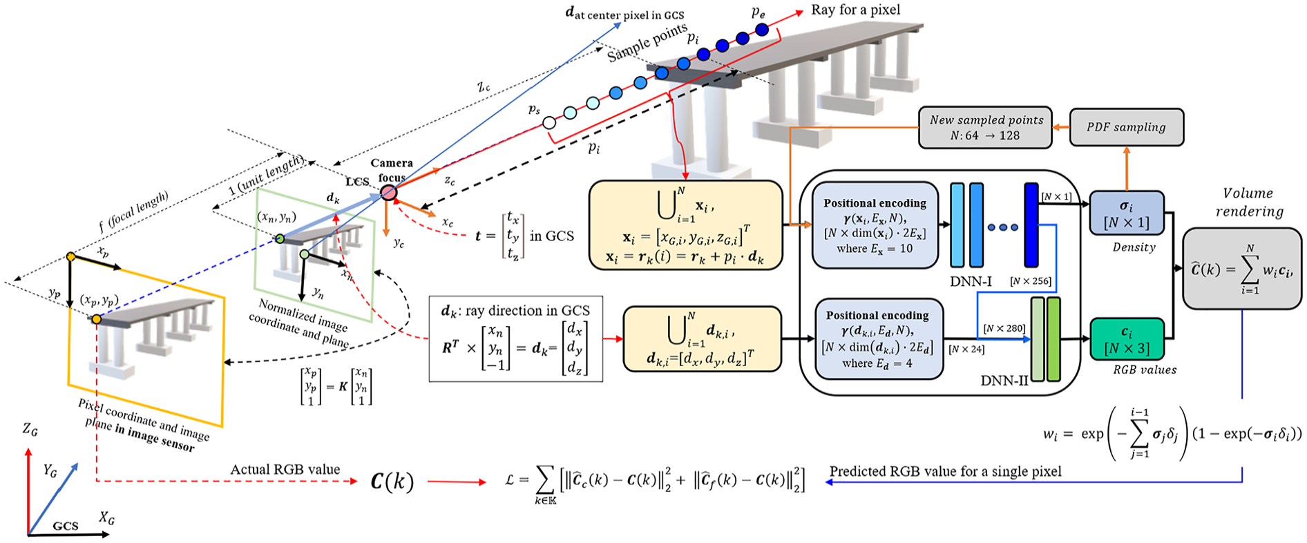
Overview of the NeRF model.
Using these various sample points, which have different distances between the camera and the object and are in the same line of the specific ray for each pixel, the NeRF model, which has DNN-I and -II, can learn the actual color in terms of RGB of the specific pixel through various collected images that have different fields of view, directions, and distances between the camera and the object of interest in GCS. To improve the model’s accuracy, new 3D sample points are created during the DNN-I process by employing density-weighted probabilities via probability density function (PDF) sampling. These newly generated sample points are subsequently utilized to retrain the model, aiming to achieve a more precise RGB value for the specified pixel. The initial and subsequent phases are referred to as a coarse process and a fine process using PDF sampling, respectively.
Therefore, through a simple cost function, the predicted RGB values from the coarse and fine processes of NeRF will be compared with the actual RGB values coming from the collected image. Following that, through backpropagation, the DNNs will be trained to predict RGB values for different distances and directions for a more accurate establishment of the 3D model for the structures of interest. The detailed steps for the NeRF will be explained in the subsequent sections.
Extraction of sample points coordinates and directional vectors in GCS
Within the model, the 2D pixel coordinates
The unit directional vector
The subsequent step involves deriving 3D coordinates for the sample points situated along a particular ray in the GCS. NeRF presets the number of sample points to (
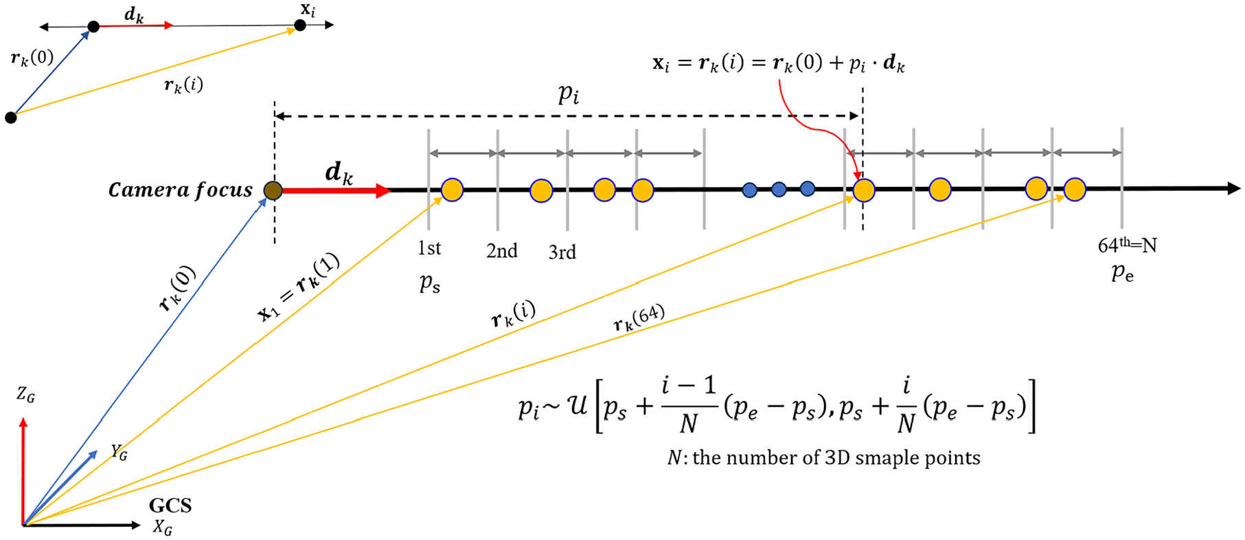
Stratified sampling along the ray.
Thus, within each ray’s path, the sample points are uniformly allocated according to Equation (9):
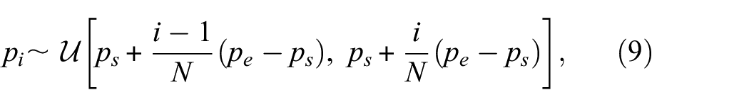
where (
Once each distance (

where
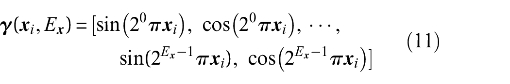
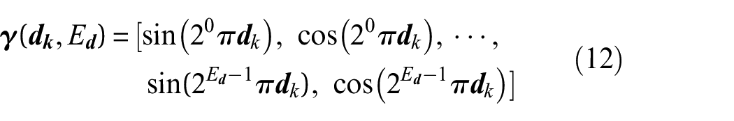
Through this positional encoding, by enhancing the model’s sensitivity to subtle variations in geometry and appearance, NeRF is capable of learning RGB values across a diverse range of distances and angles, enabling the production of photorealistic images.
DNN-I and DNN-II for prediction of RGB color and density
The expanded inputs
Figure 7 illustrates the architectures of DNN-I and DNN-II. These DNNs consist of fully connected layers with 256 and 128 neurons, respectively, followed by rectified linear unit (ReLU). Specifically, after the
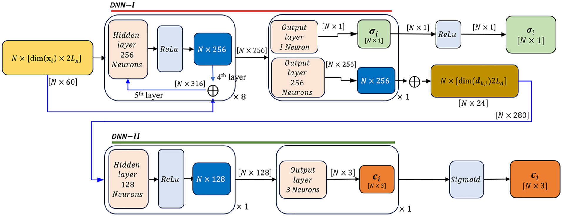
The architectures of DNN-I and -II in the NeRF Model.
Afterward, the expanded input (
Volume rendering and loss function
In the NeRF model, each 3D point’s color and density along a ray contribute to the final image color, processed through a volumetric rendering function as shown in Figure 5. This volume rendering function calculates the RGB color at the
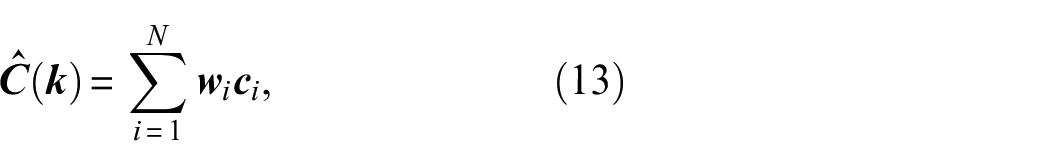
where
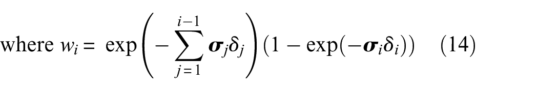
The first term
The second term
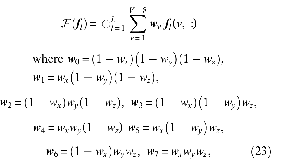
Overall, combining these terms, the weight
PDF sampling and loss function
As shown in Figure 5, for density value prediction, two separate sampling methods, coarse and fine, are implemented. The different density values obtained are then used to calculate separate predicted (
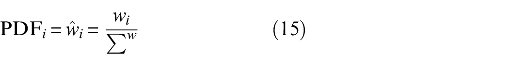
The PDF sampling process incorporates a PDF for normalization, as outlined in Equation (15):
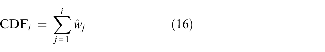
Subsequently, the cumulative distribution function (CDF) is used to calculate cumulative values, as shown in Equation (16):
Following this, 128 random values are generated, (
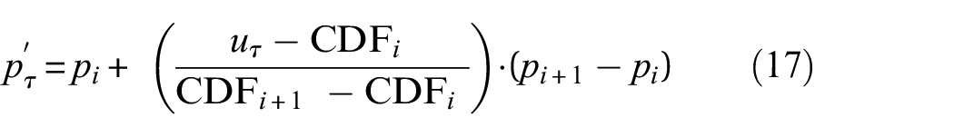
This PDF sampling method generates new distances
Finally, using the two predicted values (
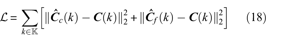
where
From this methodology, it’s understood that having a larger number of similar images of an object increases the likelihood of consistently observing the same color. This consistency in color observation is vital as it leads to a higher weighting in the training process, thereby improving the accuracy of the model’s actual color representation.
Nerfacto model
As we discussed above, the original NeRF model faces several limitations: (1) Computational efficiency: NeRF requires significant computational resources due to the large number of parameters in the DNN and the high number of samples per ray, making it slow to train and render, (2) Memory usage: The large DNNs and the need to store many samples per ray leads to high memory consumption, (3) Training speed: The original NeRF is slow to train due to its large DNN and the high number of samples per ray, and (4) Flexibility and adaptability: NeRF model’s original architecture limits its adaptability to different types of scenes and datasets.
To overcome these limitations, the Nerfacto model adopts proposal sampling from Mip-NeRF 360 to efficiently sample 3D points, multiresolution hash encoding from Instant-NGP to replace the positional encoding of
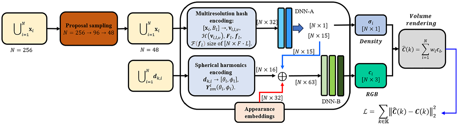
Nerfacto model architecture.
Proposal sampling
The traditional NeRF sampling process involves uniformly sample points along each ray having
Figure 9 provides a detailed view of the proposal sampling module’s architecture. This module comprises two distinct DNNs (namely, DNN-α and DNN-β), each consisting of three layers. Initially, the input (
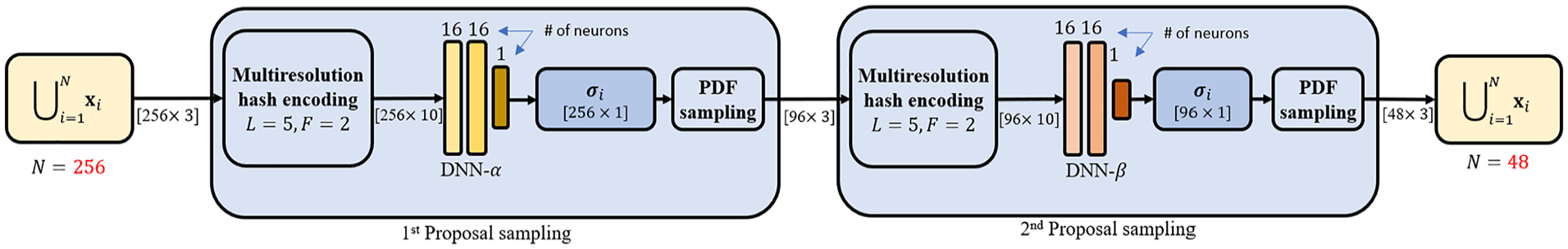
Proposal sampling network structure.
By leveraging this method, the proposal sampling approach aids in identifying high-density samples through DNNs and PDF, thereby effectively decreasing the total number of 3D sample points to
Multiresolution hash encoding
In traditional NeRF, pipelines as described in the previous section, the input dimensions of the positional encoders are determined by
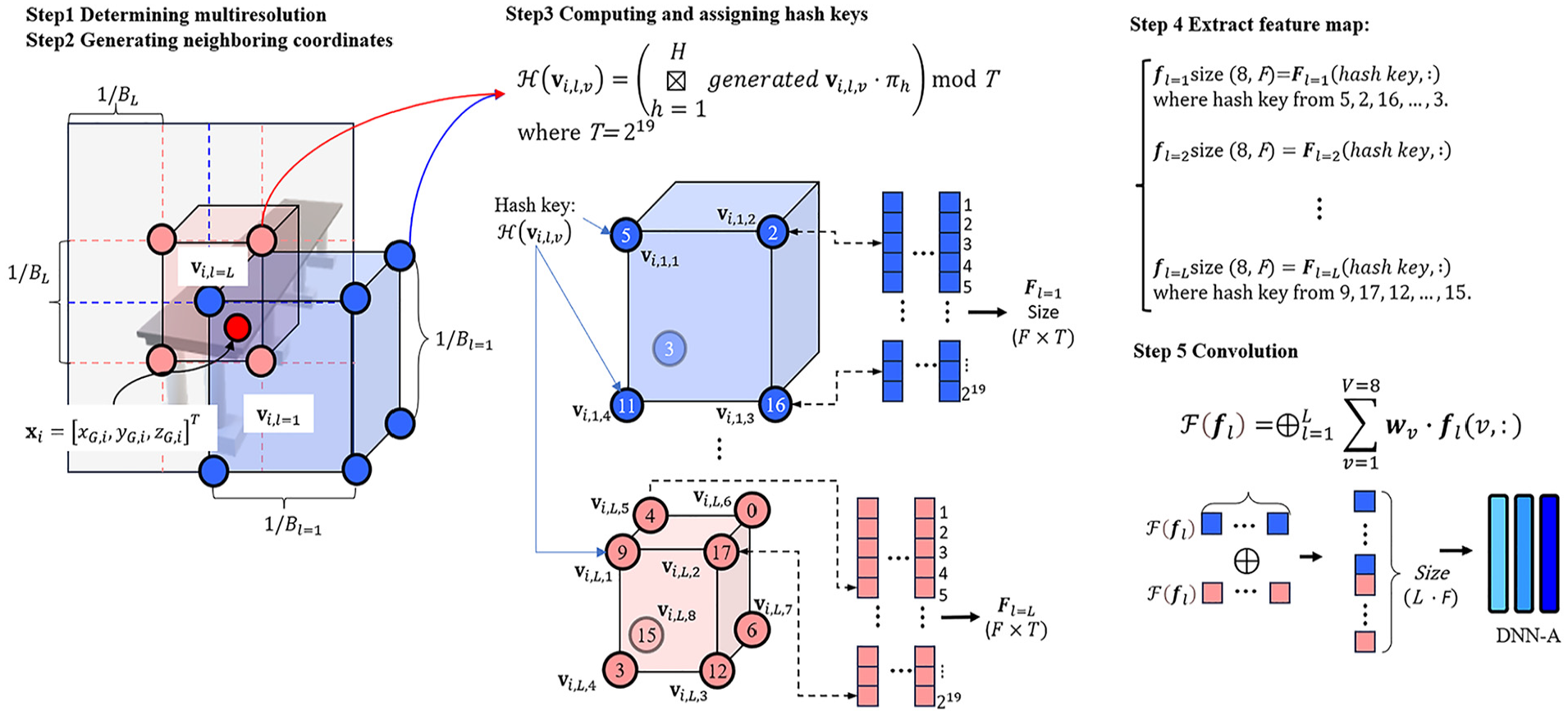
Schematic view of the multiresolution hash encoding process.
As shown in Figure 10, as the first step, in a 3D space of

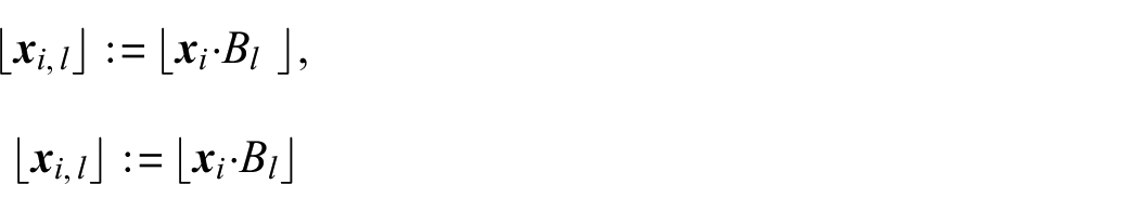
where ⌊·⌋ denotes the floor function, := means that “it defines”,
where
For a given 3D sample point having
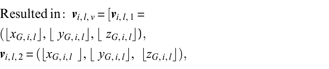
where ⌊·⌋ and ⌊·⌋ denote the floor and ceiling functions, respectively, applied to the scaled coordinates to derive the integer indices of the voxel vertices, and
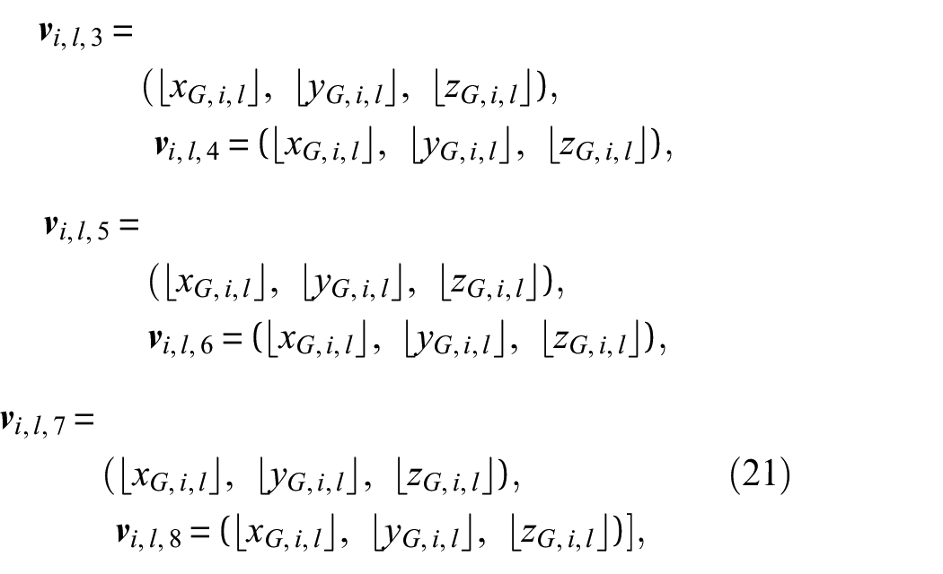
As shown in Figure 10, these eight generated coordinates are then converted into hash key values
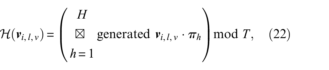
where
To compute the final feature vectors,
where
where
The use of hash encoding in the Nerfacto model significantly enhances computational efficiency by reducing the granularity of data that the DNN processes, without compromising the integrity of spatial information. This method enables the handling of large-scale environments and complex geometries more effectively due to its multiresolution approach and efficient memory usage. However, while hash encoding effectively manages spatial data, it does not inherently account for the complex interactions of light and color in a scene in terms of different viewing directions, which are crucial for achieving photorealistic renderings. This leads the Nerfacto model to incorporate spherical harmonics encoding.
Spherical harmonics encoding
The Nerfacto model uses spherical harmonic functions to generate the input for the DNN-II using the viewing direction
The value,
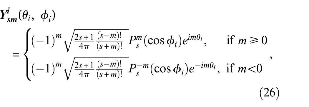
where s is the degree of spherical harmonic function (in Nerfacto, s = 3),
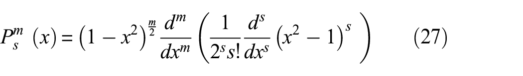
For a given degree
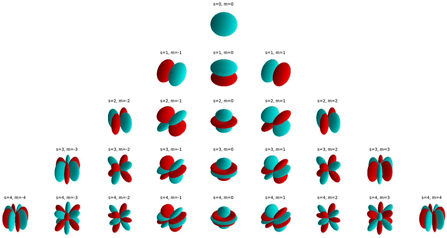
Visualization of spherical harmonic functions.
For example, (s = 0, m=0), (s = 1, m=−1, 0, 1), (s = 2, m = −2, −1, 0, 1, 2), (s = 3, m = −3, −2, −1, 0, 1, 2, 3), which can be expressed as
To sum up, the original NeRF model employs positional encoding to extend the dimensionality of input coordinates. This encoding uses a series of sinusoidal functions to map low-dimensional coordinates into a higher-dimensional space, capturing high-frequency variations and enabling the model to represent complex patterns and details in the scene. For example, for the original NeRF model with
Appearance embedding
The original NeRF model trains its second DNN (DNN-B) using each pixel’s information independently during the backpropagation of the network, without considering the entire image context because it is a pixelwise comparison in the loss function as presented in Equation (15). This approach makes it image-independent, relying solely on the ray direction and position for color prediction. This structure may cause the model to misinterpret features when there are images of the same object taken under different lighting conditions, potentially resulting in artifacts or inconsistencies in the 3D reconstruction.
In contrast, the Nerfacto model incorporates an additional input for the DNN-B that is the appearance embedding. This additional technique enables Nerfacto to handle varying conditions within the training dataset, such as different lighting setups, as shown in Figure 12. The appearance embedding generates a feature vector
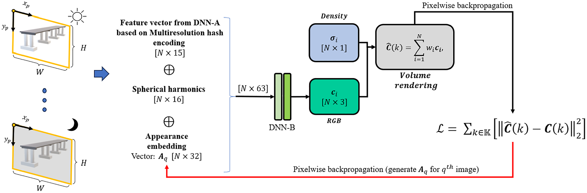
Visualization of the appearance embedding process.
It is concatenated with the outputs from the spherical harmonics of the ray direction
Data
The foundation of any successful structural damage identification and 3D reconstruction project lies in the quality of the data acquired. This section discusses the data used in STRNet with TTA for crack segmentation and the data used in 3D image reconstruction for 3D damage mapping, detailed in sections “Data for crack segmentation” and “3D image reconstruction including damage mapping,” respectively.
Data for crack segmentation
For damage segmentation, the pretrained STRNet was utilized. STRNet was trained using diverse datasets with varying resolutions (1024 × 512 and 1280 × 720), initially acquired by Kang and Cha, 21 the developers of STRNet. Table 1 provides details on the number of images and their sizes for each case.
Datasets for crack segmentation case studies.
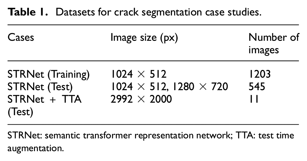
STRNet: semantic transformer representation network; TTA: test time augmentation.
3D image reconstruction including damage mapping
To generate a 3D image reconstructed model, high-quality RGB images of the structure of interest are required. As discussed in section “Camera parameter extraction,” each image has its own local coordinate system (LCS) that must be converted to the global coordinate system (GCS) for the 3D reconstructed model in the Nerfacto model. Intrinsic and extrinsic parameters (

Markers.
These markers, created with Metashape software, were carefully positioned on the top, bottom, and sides of the bridge, as depicted in Figure 14. They serve a dual purpose: providing precise reference points for the coordinate system and scale definition and facilitating effective camera alignment by providing a unique feature of each marker in each image. The markers, which are coded targets, were placed in the scene prior to taking photos. They were then utilized within the photo scan software, not only as reference points but also as crucial elements in the image matching process, particularly through the “Align Selected Cameras” feature. Adhering to best practices, we ensured that each captured image included at least one marker. This method greatly enhanced feature matching and spatial orientation, a critical aspect in photogrammetry. The use of markers proved especially advantageous for the Nerfacto technique, as it provided highly accurate camera pose estimations, crucial for precise 3D reconstruction.
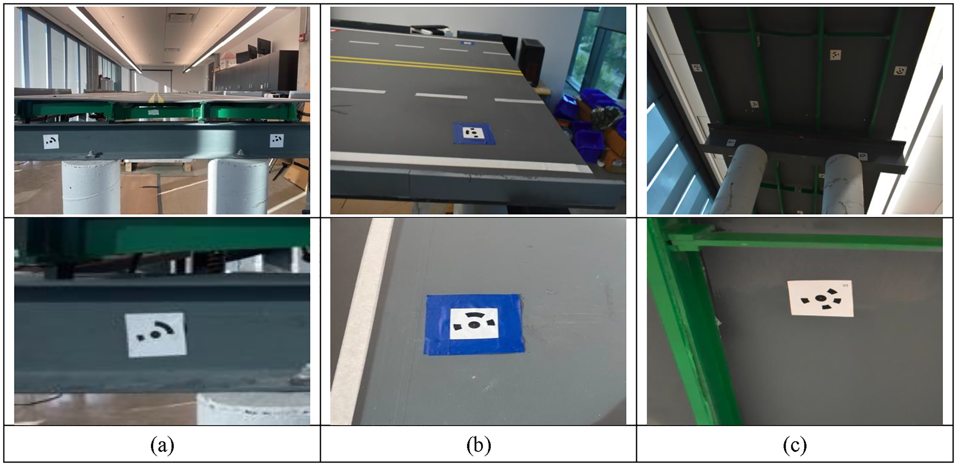
Aligned Markers on the bridge. (a) Front view of the bridge. (b) Top view of the bridge and (c) Bottom view of the bridge.
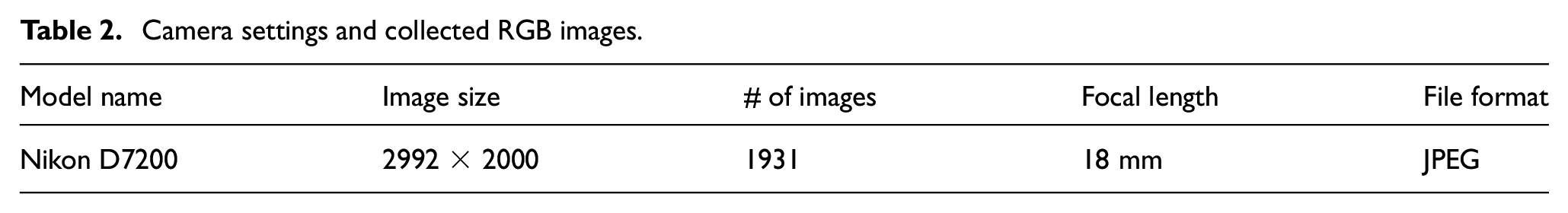
To obtain high-resolution images, we used a Nikon digital camera. Table 2 details the camera settings used for data collection and the total number of images collected as input for Nerfacto for 3D reconstruction. To balance image quality with computational efficiency, we selected a resolution of 2992 × 2000 pixels and a focal length of 18 mm. Additionally, we chose the JPEG fine image format to balance image quality and file size, ensuring manageable data for subsequent processing stages. These settings ensured each image size was less than 5 MB, capturing high-quality images while considering computational constraints.
Camera settings and collected RGB images.
The process of capturing these images for 3D reconstruction involves meticulous attention to detail. Each photo was taken to capture the desired features of the bridge model, with close-ups ensuring that many image pixels represent the bridge. The experiment was conducted in the lab, as shown in Figure 15. To obtain an accurate 3D model, each image contained at least one marker, and significant emphasis was placed on image overlap, ensuring that each image overlapped with its neighboring images by at least 80%.
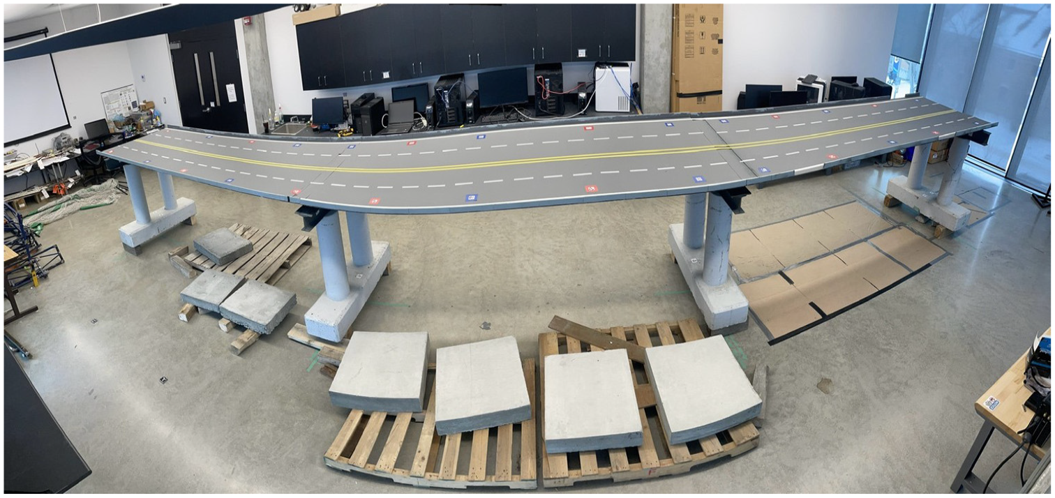
Panoramic view of the structure of interest.
Case studies
In this section, we conduct extensive case studies to evaluate the performance of crack segmentation and subsequent 3D damage mapping on the 3D reconstructed model. These case studies aim to provide a comprehensive understanding of the various factors that affect the quality and accuracy of crack segmentation and 3D reconstruction for damage mapping.
Section “Crack generation and computing power” briefly describes the method used to induce cracks in real concrete bridge piers and outlines the computing power required for STRNet with TTA and Nerfacto simulations. Section “STRNet + TTA evaluation” details the various training and testing modes of STRNet with TTA techniques to achieve state-of-the-art results in crack segmentation, measured in terms of mean Intersection over Union (mIoU). Section “3D reconstruction and damage mapping using Nerfacto” presents various case studies for training the Nerfacto model and their results, including traditional methods of 3D reconstruction. Extensive comparative studies were conducted to demonstrate the effectiveness of our approach.
Through these case studies, we illustrate a real-world application of our integrated SHM approach, which combines advanced deep learning techniques for damage detection and 3D reconstruction for 3D damage mapping to create a digital twin with segmented damage information.
Crack generation and computing power
The bridge system used in this study has the following dimensions: a bridge deck width of 118 cm, a length of 921 cm with three simply supported deck systems, and a height of 124 cm for the bridge piers, including the thickness of the bridge deck. Cracks were induced in the bridge piers using a pressure machine to simulate damage, as illustrated in Figure 16. To conduct damage segmentation and 3D mapping on the 3D reconstructed model, we used a high-performance computer equipped with an AMD Ryzen 3990x CPU and an Nvidia RTX A6000 GPU, running on Ubuntu 20.04.6 LTS OS. For the Nerfacto model, we employed the Nerfstudio framework.
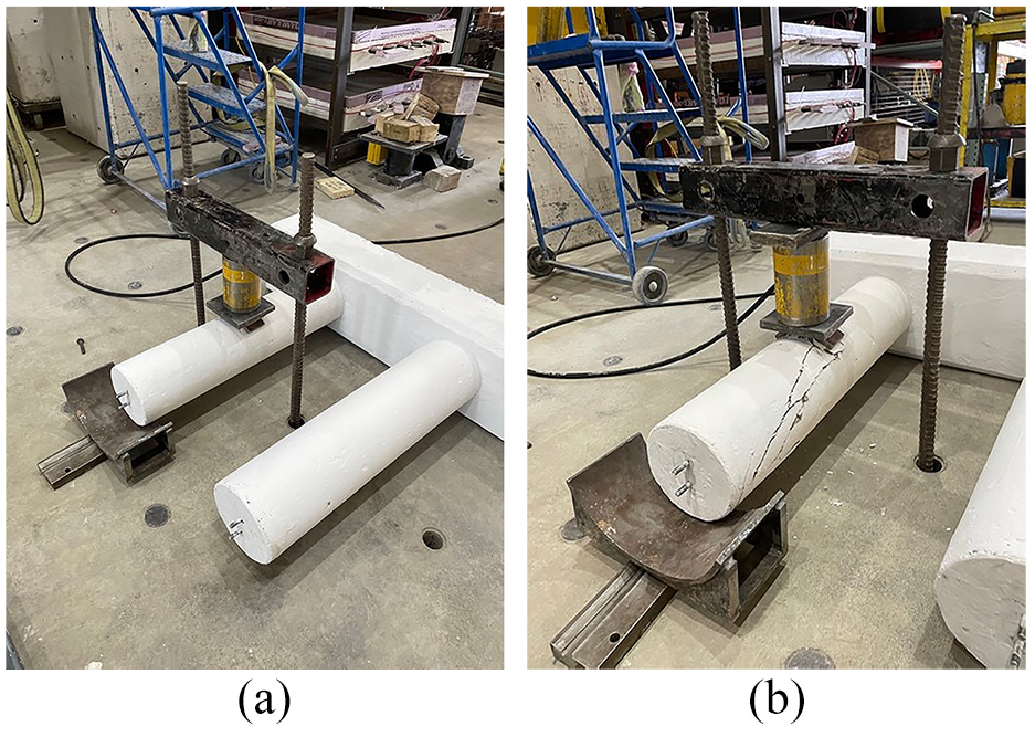
The process of creating cracks on the bridge pier. (a) Before creating cracks and (b) after creating cracks.
STRNet + TTA evaluation
In this article, the main focus is on 3D damage mapping through the 3D reconstruction of the bridge system. Therefore, the state-of-the-art crack segmentation method, STRNet, was employed for crack segmentation. mIoU was used as the evaluation metric to evenly consider false positives and false negatives, as presented in Equation (28).
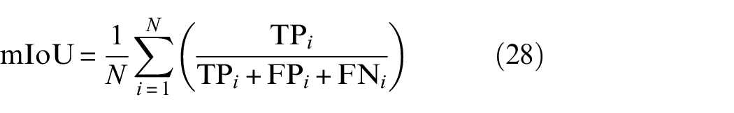
where (N) is the number of images, (TP) represents True Positives, (FP) represents False Positives, and (FN) represents False Negatives.
The STRNet was trained using the existing dataset presented in Table 1 and achieved a 92% mIoU with a dataset of 545 images at resolutions of 1024 × 512 and 1280 × 720. However, as presented in Table 3, the crack segmentation accuracy of STRNet with this new structure is slightly lower than the reported performance in the original article, 21 at 80% mIoU. This reduction in accuracy is due to the significantly different structure and its environment compared to the existing data, which were collected from outdoor structures. Therefore, STRNet was integrated with the TTA approach to improve the results.
Comparative studies: STRNet and STRNet + TTA.
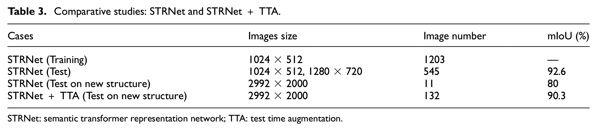
STRNet: semantic transformer representation network; TTA: test time augmentation.
For the TTA, 12 different augmentation methods were conducted, including resizing, vertical and horizontal flipping, and rotations of 90°, 180°, and 270°. Through these augmentations, a total of 132 testing images were generated and tested. STRNet with TTA increased the mIoU to 90.3% with the new testing set of 132 images, excluding the 545 existing testing images from the original paper. 21 Cracks on the pillar were specifically selected to evaluate the mIoU for both STRNet and STRNet with TTA for this structure of interest.
Figure 17 visually demonstrates the performance of STRNet and the effects of TTA on crack segmentation accuracy through real cracks on the structure of interest. The figure shows the results of segmented cracks in the bridge piers and compares the traditional STRNet results with those of STRNet with TTA. As indicated by the blue-lined circles in the STRNet results, there are significant improvements in crack segmentation overall when using STRNet with TTA. These improvements stem from the nature of TTA.
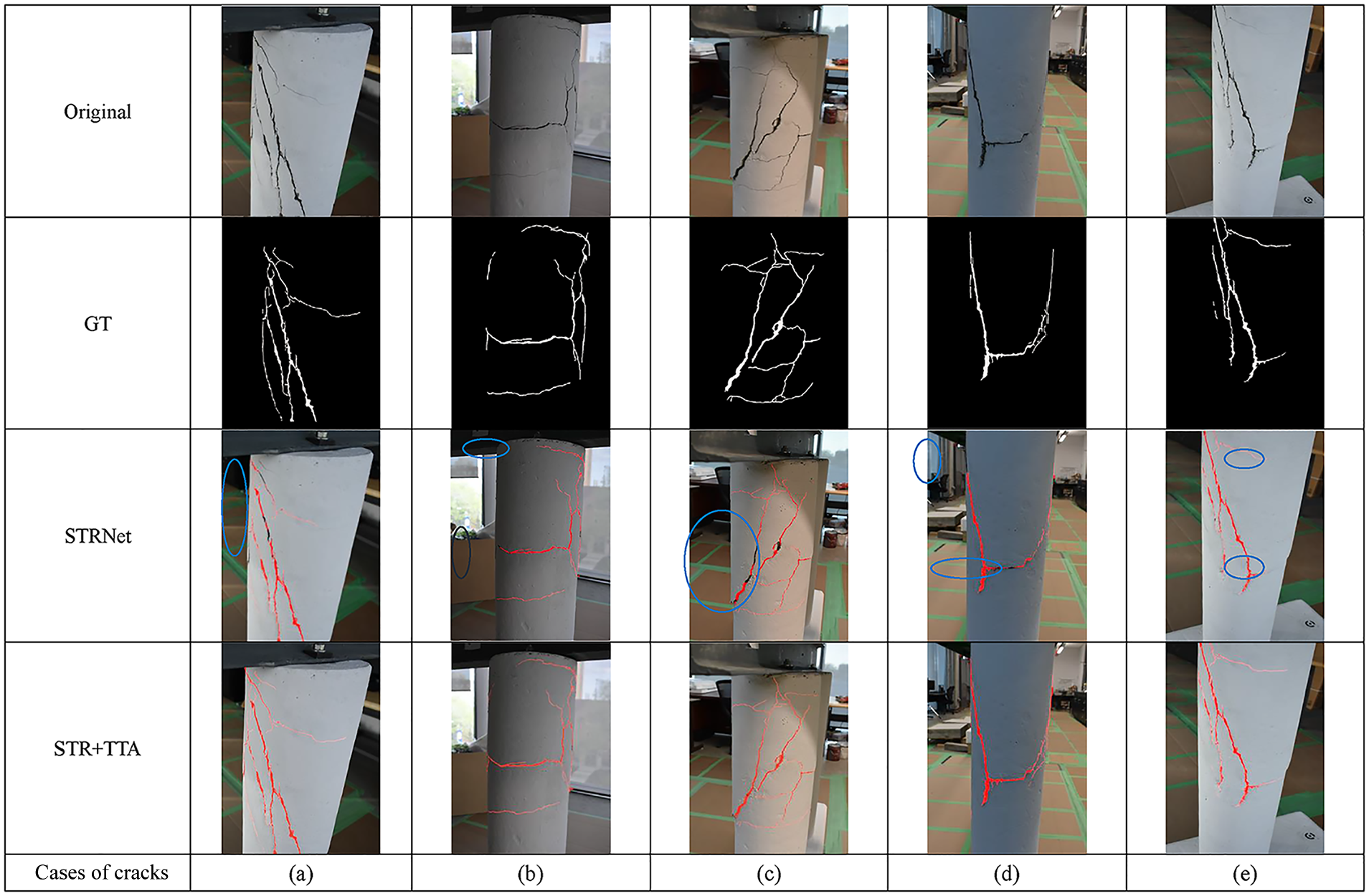
Crack segmentation results using STRNet and STRNet + TTA.
TTA augments the input image in various ways, as described in section “Test time augmentation.” The augmented input images are then fed into the trained STRNet, and all the results from the augmented input images are unified together. The unified results are presented as the final output. In this way, very thin cracks and missed cracks, which might be overlooked for various reasons, have a chance to be detected at least once, contributing to the final results. Consequently, STRNet with TTA achieved a 90.3% mIoU, as presented in Table 3.
Moreover, the minimum detectable crack width per pixel is contingent upon factors such as camera resolution, focal length, sensor type, lens characteristics, including the performance of our segmentation model and the characteristics of the data used for training the STRNet. Our test dataset labels were meticulously annotated down to individual pixels on high-resolution images (2992 × 2000 × 3), facilitating precise crack detection. Nonetheless, determining the minimum detectable crack width at significantly greater distances was beyond the scope of this study, as it would adversely affect the quality of the 3D reconstruction, which is the primary focus of the research. We determined that maintaining a camera distance of 1 to 2 m provides an optimal compromise between detailed crack detection and high-quality 3D reconstructions.
Figure 18 demonstrates the precision of pixel-level crack segmentation through progressively magnified views of the same area on a column. Each image in the sequence captures increasingly detailed aspects of the segmented cracks.
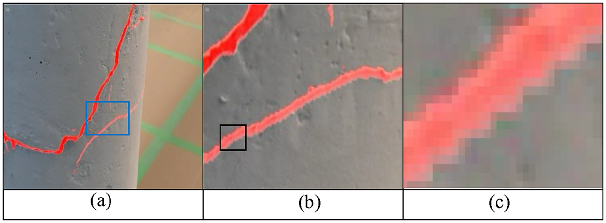
Progressive zoom levels of crack segmentation.
3D reconstruction and damage mapping using Nerfacto
The NeRF and Nerfacto techniques introduced in section “Data” are available within the Nerfstudio framework 45 to facilitate 3D reconstruction. Nerfstudio is a modular PyTorch framework known for its extensibility and versatility in neural radiance field development. It consolidates various NeRF techniques into reusable, modular components, enabling real-time visualization of 3D reconstructed scenes, offering comprehensive controls, and providing a user-friendly, end-to-end workflow for creating diverse NeRF-based models from user-captured data. As an open-source project, Nerfstudio benefits from ongoing enhancements contributed by both academic and industry experts.
Through trials, we found that the original NeRF model was not suitable for our structural case due to its rendering limitations, including excessively high computational costs, which resulted in excessively long training times for the DNNs within NeRF, ultimately causing the training process to be halted. Therefore, in this paper, we extensively investigated Nerfacto through various parametric studies, including modifications to its DNNs and methods of collecting RGB image data, to improve 3D reconstruction and damage mapping.
As an initial step, the collected RGB input images were fed into the Nerfstudio framework. It rendered the global distributions of the entire RGB input images, as presented in Table 2, with their corresponding global locations determined from the intrinsic and extrinsic parameters that were extracted from Metashape, as shown in Figure 19.
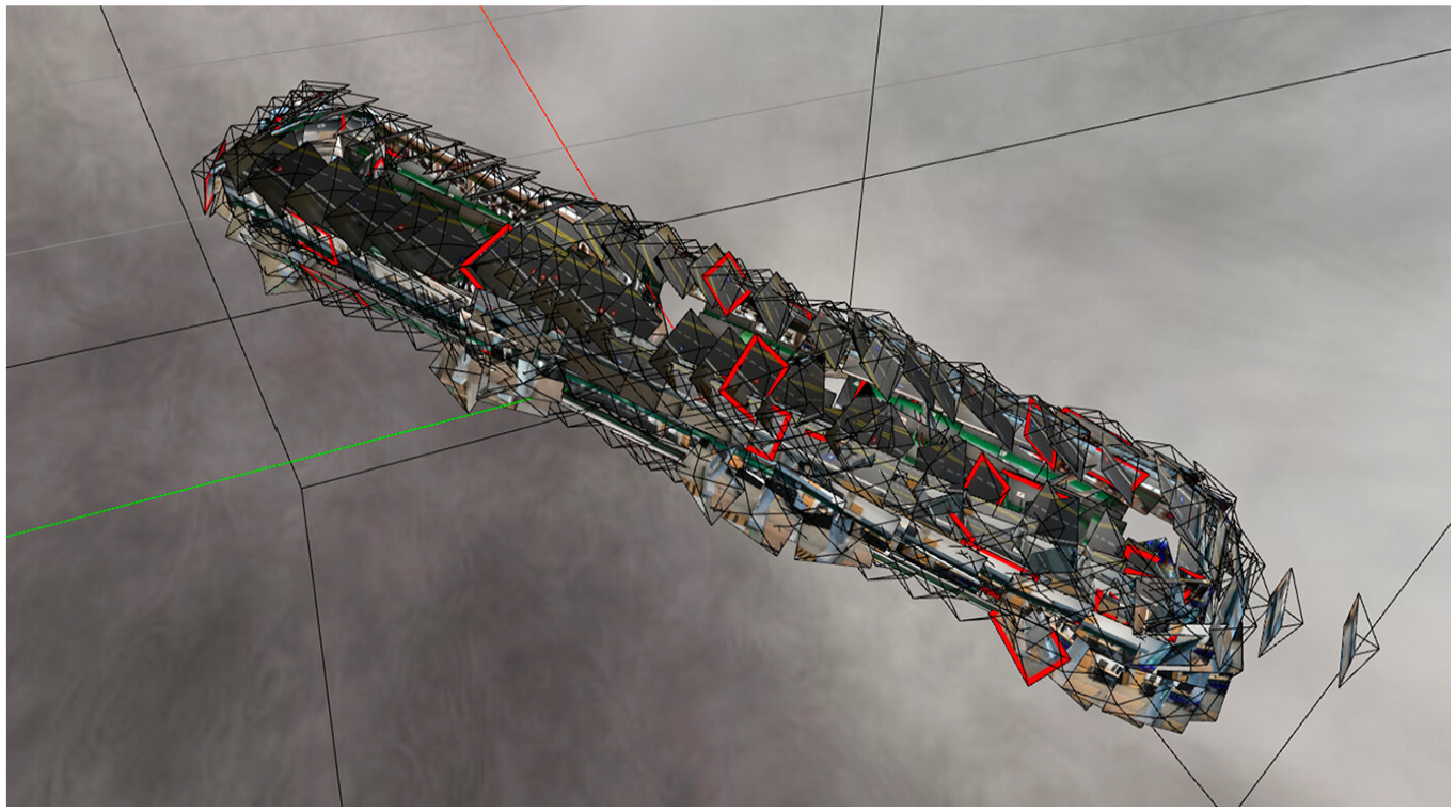
Global distributions of all input images based on the estimated camera poses using intrinsic and extrinsic parameters.
Using the default hyperparameter settings, the web URL provides a real-time rendering of the model’s training progress. Initial renderings appear blurry, as shown in Figure 20(a), but gradually become clearer as the model's color training progresses, as shown in Figure 19.
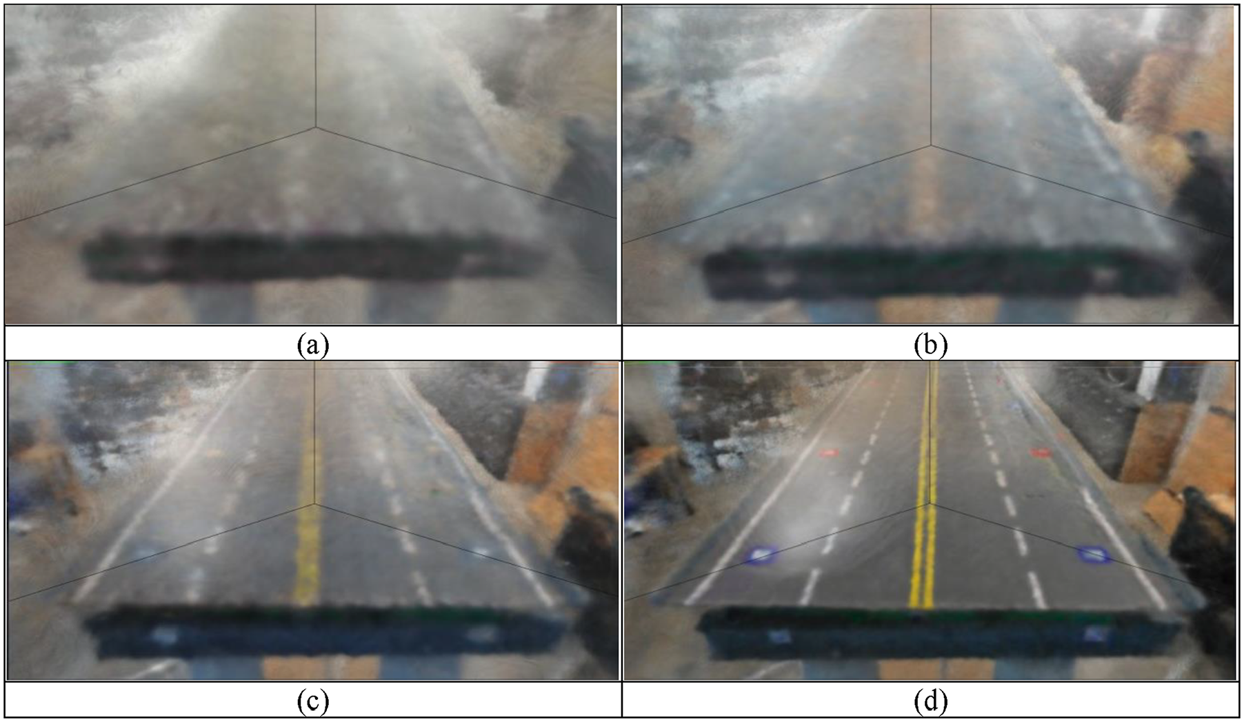
Real-time training progress of Nerfacto is displayed on a web URL. (a) Iteration 300. (b) Iteration 700. (c) Iteration 1000 and (d) Iteration 2000.
Parametric studies of Nerfacto
In this section, core evaluation metrics used for the evaluation of the 3D reconstructed model are introduced, along with various parametric studies, including modifications to its DNNs and methods of collecting RGB input image data, to examine the effects on the quality of the 3D reconstruction.
Evaluation metrics
To evaluate the results of the 3D reconstruction through the extensive parametric studies, several evaluation metrics were adopted. These included the MSE loss function, Peak Signal to Noise Ratio (PSNR), and Structural Similarity Index (SSIM), which are essential for assessing the quality of the rendered images. 45
PSNR measures the ratio between the maximum possible signal value and the distorting noise affecting its representation, providing insights into the fidelity of the reconstruction. It is calculated using Equation (29):

SSIM, on the other hand, is a method for predicting the perceived quality of images, considering factors like luminance, contrast, and structure. SSIM is calculated using Equation (30). Both PSNR and SSIM are popular metrics in the field; however, each metric has its limitations. Therefore, employing all three metrics, including MSE Loss, offers a more comprehensive assessment of our 3D reconstruction quality.
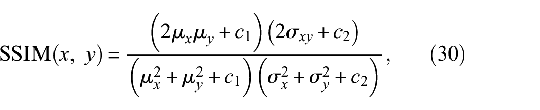
where
PSNR measures the peak error between the reconstructed and original images, providing a quantitative measure of the reconstruction’s precision in terms of pixel intensity errors. This metric is crucial for understanding the technical accuracy of the model’s output relative to the ground truth. Conversely, SSIM evaluates the visual perception of the reconstructed images by analyzing changes in luminance, contrast, and structure compared to the original images. This metric offers insights into the perceptual impact of our reconstruction process, addressing aspects of image quality that PSNR does not capture, such as visual fidelity and textural preservation.
The use of both metrics is standard in NeRF-related research because they together offer a comprehensive overview of both the objective accuracy and subjective quality of the reconstructed images.
However, as Tancik et al. 45 point out, these evaluations are typically based on images that follow the same capture trajectory as the images used for training. This approach can be misleading, especially in real-world applications that capture data from unstructured environments and render new views with significant deviations from the training set. Relying solely on PSNR and SSIM might not fully reflect the model’s performance in diverse and practical scenarios.
It is important to recognize that while metrics such as PSNR offer some insights, they do not encompass a complete understanding of a model’s performance, particularly for views that diverge substantially from the capture trajectory. A more holistic approach involves qualitative evaluation, such as using an interactive viewer, which can provide a deeper and more comprehensive understanding of the model’s capabilities in various conditions. Despite these considerations, quantitative metrics still hold value in certain aspects of our analysis.
Parametric studies including modification of DNNs
In this section, various parametric studies were conducted, and the performance of the Nerfacto was compared to some existing 3D reconstruction methods, including the original NeRF. As an example of a traditional 3D reconstruction method, a dense point cloud and mesh-based method using photogrammetry software was implemented. This method was presented as Case 1 (C1) in the results table (Table 4). For Case 2 (C2), the original NeRF model was implemented. In Case 3 (C3), the effects of relatively lower input image resolution were investigated. For Case 4 (C4), higher resolution with a relatively smaller number of input images was also investigated. In Case 5 (C5), the methods of collecting input images were investigated. In this case, two different methods of collecting the input images were implemented, as shown in Figure 21.
Comparative and parametric studies.
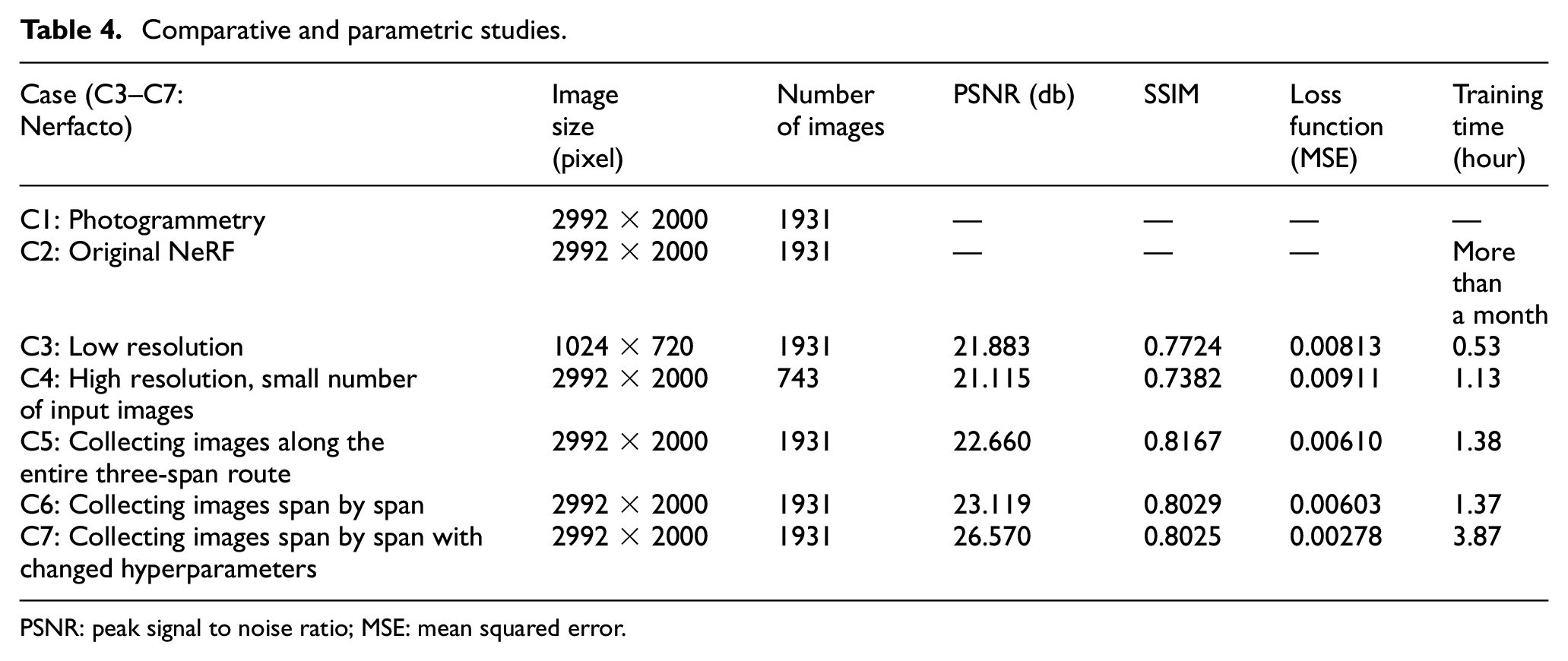
PSNR: peak signal to noise ratio; MSE: mean squared error.
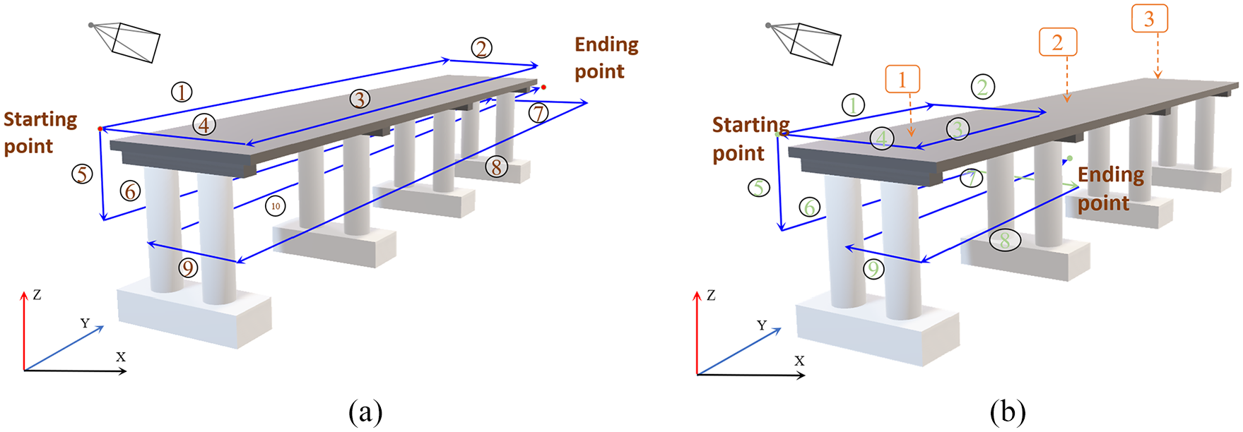
Photography routes. (a) Entire three-span route of photography and (b) each span route of photography.
As illustrated in Figure 21, the three bridge deck spans were scanned along the entire three-span route by moving back and forth, with the images assigned numbered starting and ending points. Another method of collecting input images, Case 6 (C6) in the results table (Table 4), was to scan each span separately. In these two image collection methods, the same total number of 1931 images was used, and efforts were made to capture the images at similar locations and angles to isolate the effects of the collection order. The final case, Case 7 (C7), used the span-by-span image collection method, which was selected based on the results and additional parametric studies of the Nerfacto model. The final results for this case are reported in Table 4.
As presented in Table 4, the traditional photogrammetry-based method has fundamentally different mechanisms for the final 3D reconstruction, so the evaluation metrics used for the Nerfacto model cannot be directly applied. Therefore, the final result of the photogrammetry-based method is presented only in Figure 22. The original NeRF was also implemented using the same input image data, but due to its high computational requirements, the simulation was stopped after 20 days of training. We concluded that the original NeRF cannot be effectively implemented for large-scale civil infrastructure problems.
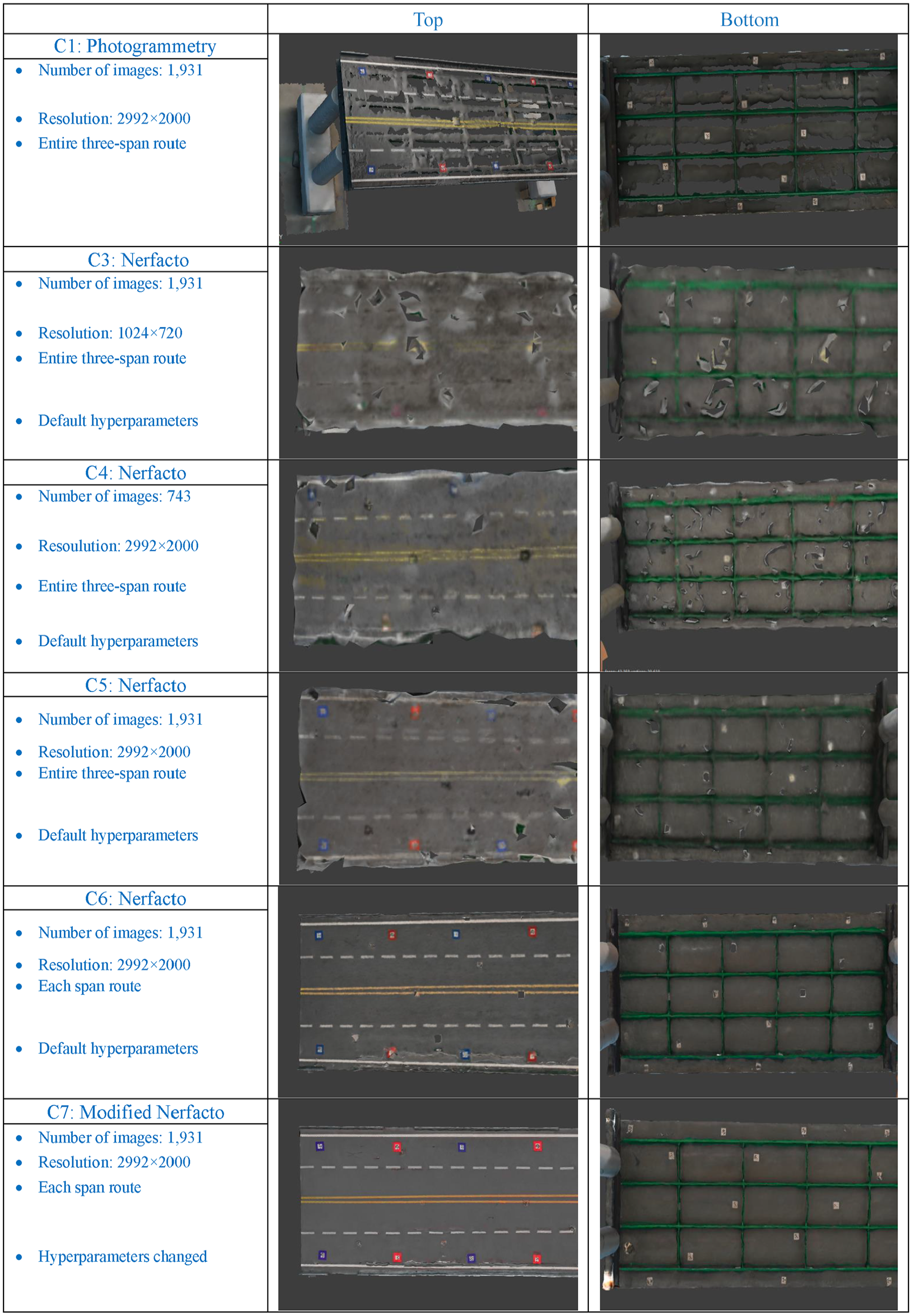
The 3D reconstruction results of each case.
From C3 to C7, the Nerfacto model was investigated extensively. In C3, relatively lower-resolution input images were used, resulting in degraded evaluation metric values compared to C4–C7. This suggests that high-resolution input images are beneficial for creating high-quality 3D reconstructed models. In C4, high-resolution images with a much smaller number of input images were used to train the Nerfacto, and the results were still slightly better than those of C3 with a much greater number of input images. Through C5 and C6, we found that the order of image collection affects the final 3D reconstruction result. The conclusion is that input images should be collected in a grid or segment-based manner to help the embedded DNNs learn the geometry of the 3D spatial structure.
As the final case study (C7), the Nerfacto model was modified with deeper DNN-A and DNN-B networks, more training iterations, a larger training batch size in terms of the number of rays processed, and a greater number of 3D sample points per ray using uniform random sampling, as presented in Figures 8 and 9. Additionally, the number of 3D sample points per ray for the proposal sampling and DNN-A was increased, as shown in Figure 9. Therefore, the modified Nerfacto model demonstrated the best performance in terms of the evaluation metrics presented in Table 4, including PSNR, SSIM, and MSE. All the detailed final hyperparameters of the Nerfacto model for the final result of C7 are presented in Table 5.
Hyperparametric settings for modified Nerfacto of C7.
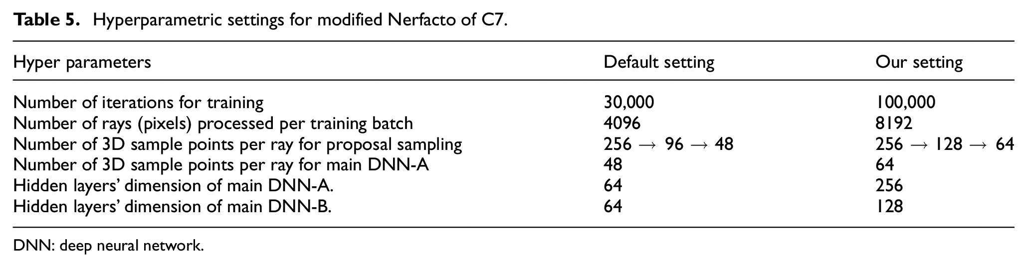
DNN: deep neural network.
The visual results of these comparative and parametric studies are presented in Figure 22. As shown in these figures, the traditional photogrammetry-based approach does not provide meaningful results in terms of resolution. The generated 3D model is too blurry and coarse to discern the structural details. The results of C4 and C5 are also not significantly different from those of C1. In contrast, C6 and C7 provide much better results with higher resolution and clearer definition of the structural members. Among these two, the result of C7 is superior in terms of the evaluation metrics presented in Table 4 and the overall visual quality. Based on these results, both in terms of the evaluation metrics and the subjective visual assessment, C7 was selected as the final Nerfacto model.
The finally selected Nerfacto model, with modified DNN architectures and adjusted hyperparameters, generated a high-definition 3D reconstruction of the entire bridge, as presented in Figure 23. The key benefits of this Nerfacto-based 3D reconstruction are that it provides a high-definition 3D model and can generate 3D views from any angle and location in real-time, optimized through the training of the DNNs. In contrast, the traditional 3D models generated by photogrammetry methods have several disadvantages. They are time-consuming to render and are limited to a single, large 3D model. Additionally, they do not allow for the generation of new 3D models from different angles and locations, which can be inconvenient for users.
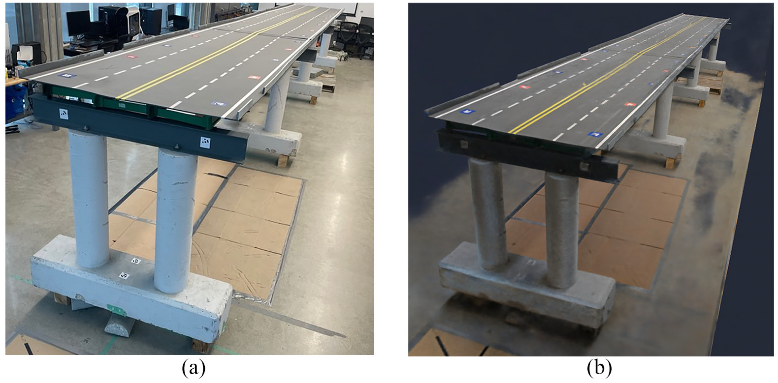
Comparison with an RGB image and Nerfacto-based 3D reconstruction. (a) Image of the bridge model and (b) 3D Reconstructed model of the bridge model.
3D damage mapping
Through the various case studies in the previous section, we found that the Nerfacto approach can generate high-resolution, clear 3D reconstructions of a large-scale bridge system. Another objective of this article is to perform 3D damage mapping of the segmented damage using deep learning models for structural damage detection. As an example, we adopted the STRNet with TTA module from the previous section “STRNet + TTA evaluation.”
To generate a 3D model with the detected damage segmented, there are two different approaches that can be used for extracting the intrinsic and extrinsic parameters for SfM, which are then used for 3D model generation using Nerfacto. Therefore, we conducted two different case studies:
Case A: In this case, we used the raw RGB input images to extract the intrinsic and extrinsic parameters for SfM, and then generated the 3D model using the intrinsic and extrinsic parameters from the raw images, combined with the damage segmented images from the STRNet with TTA.
Case B: In this case, we used the damage-segmented images from the STRNet with TTA to extract the intrinsic and extrinsic parameters for SfM, and then generated the 3D model using the intrinsic and extrinsic parameters from the damaged images. These two cases are well illustrated in Figure 24 for better understanding.
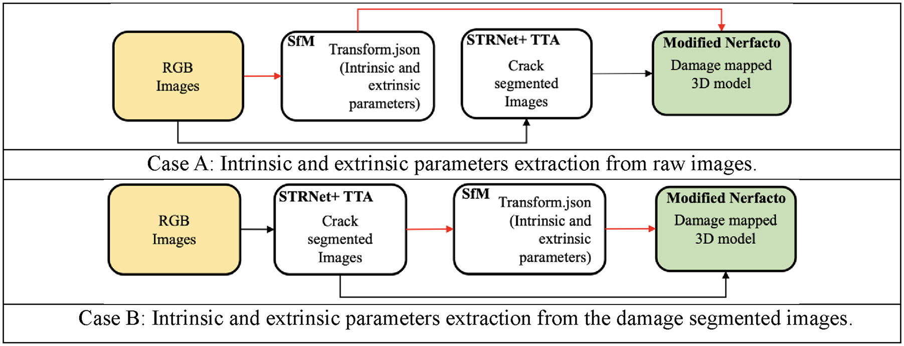
Two different approaches for extracting intrinsic and extrinsic parameters for 3D model generation. Case A: Intrinsic and extrinsic parameters extraction from raw images and Case B: Intrinsic and extrinsic parameters extraction from the damage-segmented images.
These two different approaches were compared using only 85 input images for simplified visualization, and Figure 25 illustrates the results for a specific iteration and batch. In Case A, the input pictures are well-aligned, indicating that the camera pose estimation achieved through extracting intrinsic and extrinsic parameters from the raw input images for 3D reconstruction using Nerfacto was accurate. In contrast, Case B reveals input images that are not as well aligned, suggesting that the camera pose estimation based on the damage-segmented images was less accurate.
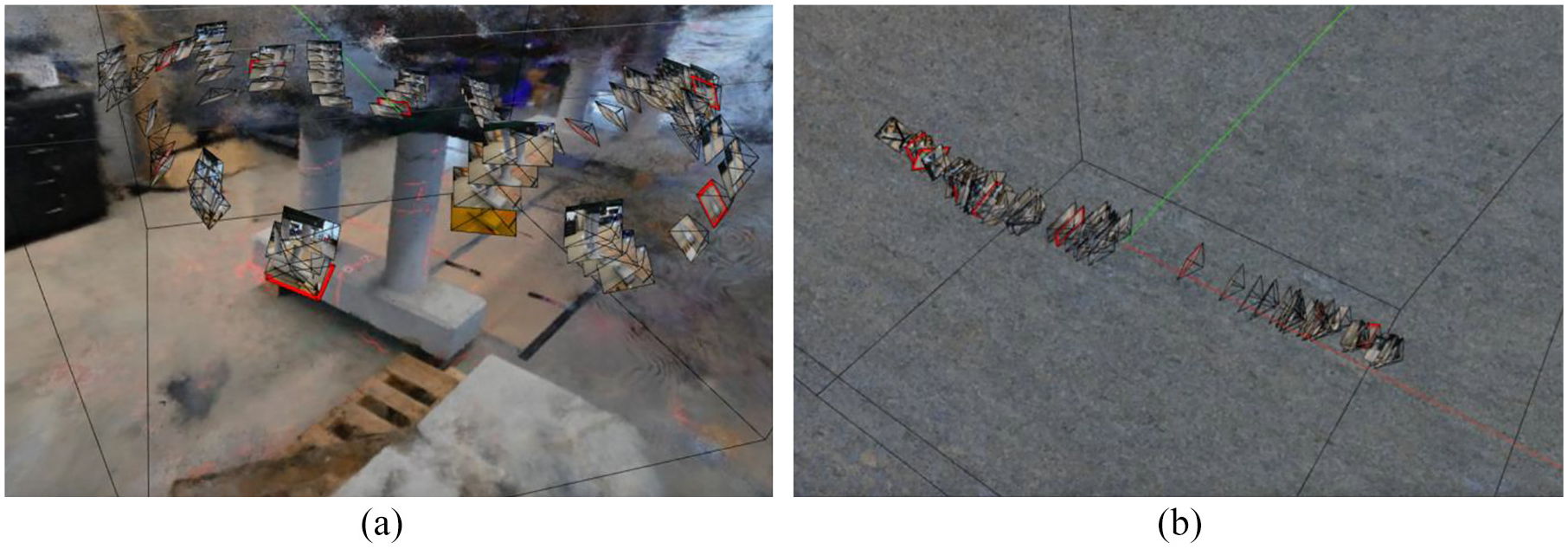
Images aligned for the camera pose estimation case. (a) Result of Case A and (b) Result of Case B.
The reason for the coarse alignment of the input batch images in Case B is that the cracks were not perfectly segmented. Therefore, during the extraction of intrinsic and extrinsic parameters using the crack-segmented images, the same objects in the input images were not accurately indicated at the same locations and angles within the parameters. This misalignment, resulting from inaccurately aligned images, leads to incorrect ray tracing from each image, which reduces the quality of the 3D reconstruction. These outcomes were observed during our tests with a set of 85 images focused on reconstructing a pair of bridge columns.
While slight variations in crack segmentation in the SfM stage can lead to potentially severe misalignment of images, this issue can be neglected during the training phase of the Nerfacto model. Nerfacto, a neural network-based model, is designed to learn from and average these variations in segmentation. The model’s training process involves optimizing network weights based on a broad set of training data, effectively allowing it to discern and emphasize the most common features in the data. Therefore, as long as the majority of the images correctly depict the segmented cracks, the model can accurately map the cracks onto the 3D structure. The example of this capacity to average out errors advantage is illustrated in Figure 26.
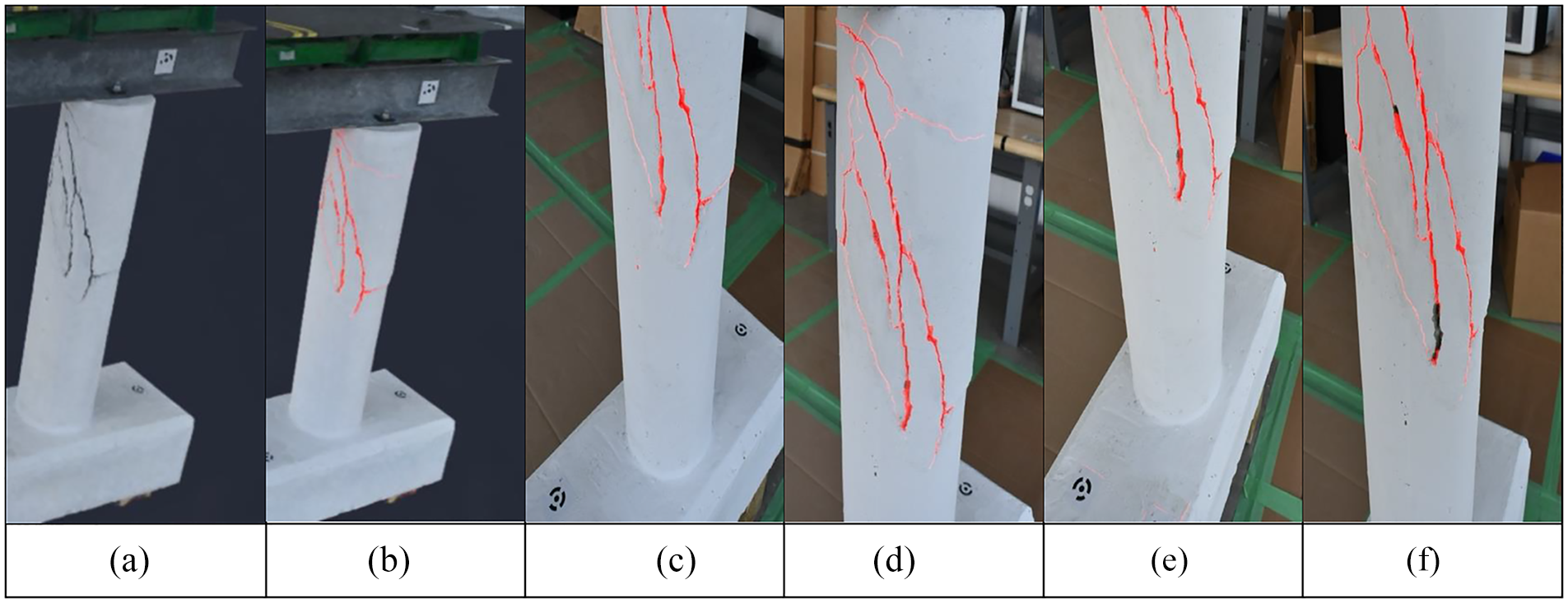
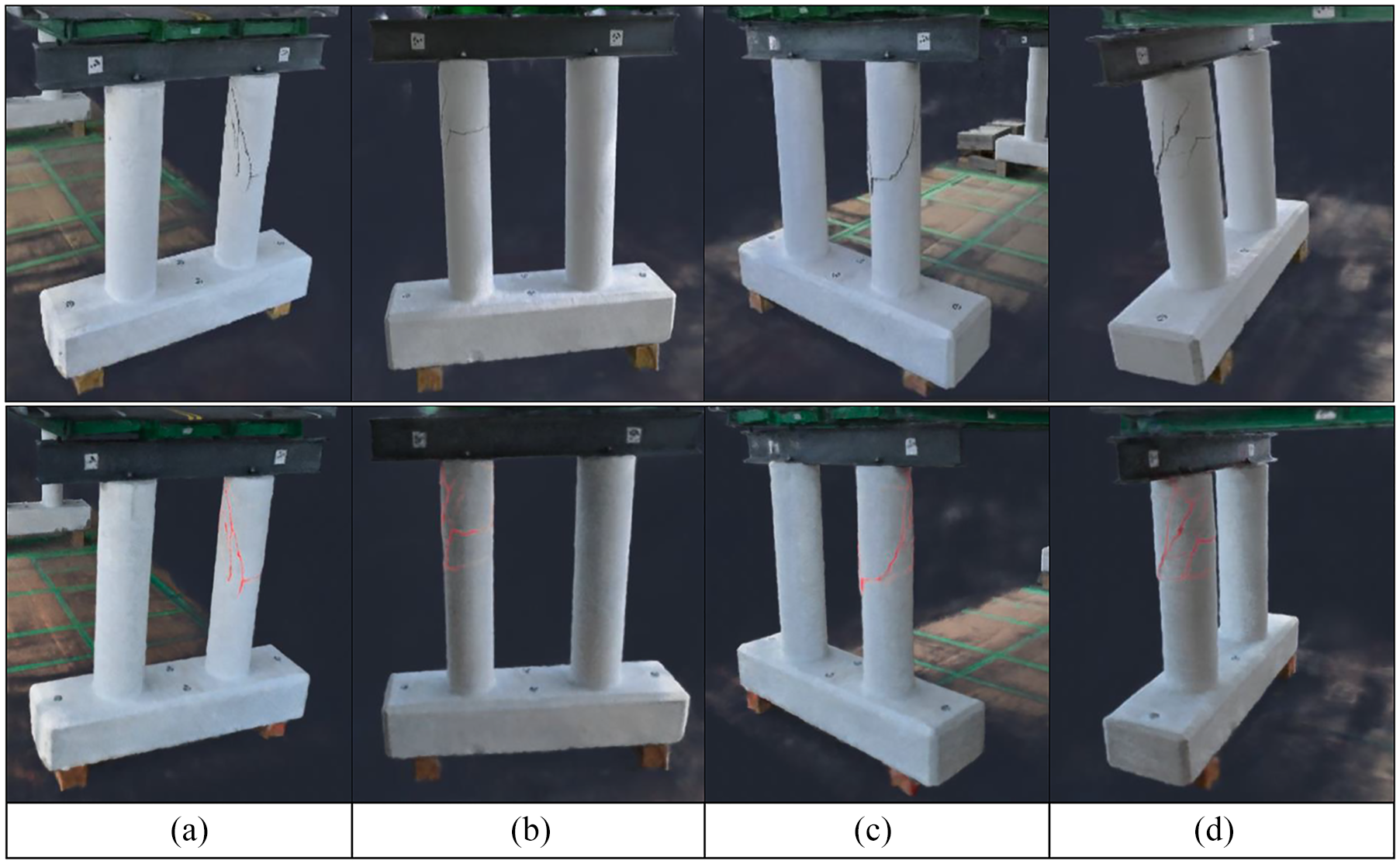
3D damage mapping consistency across varied 2D crack segmentation images. (a) Base 3D reconstruction. (b) Damage mapped 3D reconstruction. (c) Training image 1. (d) Training image 2. (e) Training image 3 and (f) Training image 4.
The 2D training images (1–4) exhibit slight variations in crack segmentation. However, the final result of the damage mapped 3D reconstructed model’s cracks shown in Figure 26(b) represents the overall average of the segmented cracks obtained during the training process. The model learns from all four training images and presents the average (i.e., predominant) values for the same area (e.g., Crack) of the structure. Image (a) displays the 3D reconstruction of a bridge pier without any damage segmentation, serving as a baseline for comparison.
Therefore, in Case A, we generated a 3D damage map using the modified Nerfacto approach with the same hyperparameters and number of hidden layers as the C7 model in Table 4. The generated 3D damage map is presented in Figure 27. This step aims to accomplish size quantification and intuitive localization of the damage on the bridge model. By visually representing the damage in a 3D context, we were able to gain a more comprehensive and realistic understanding of the structural integrity of the bridge.
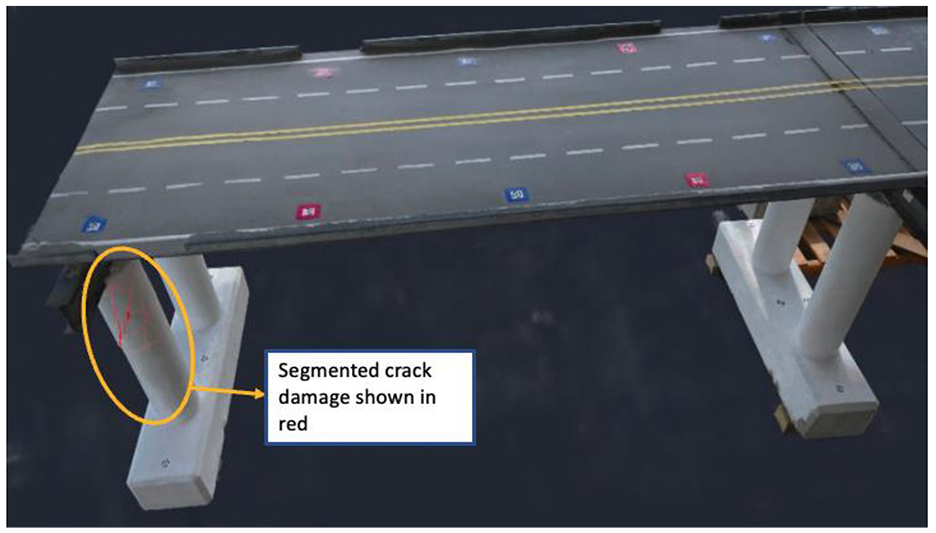
3D mapping of the segmented cracks.
A key highlight of our results is showcased in Figure 27, which presents an image of the segmented cracks mapped onto the 3D bridge model. This visual representation illustrates the accurate localization and depiction of the extent of damage to the bridge structure. The segmented cracks are clearly delineated, providing an intuitive understanding of the damage’s location and severity. Furthermore, Figure 28 offers a comparative visualization between unsegmented and segmented cracks on the 3D model. This comparison vividly demonstrates the increased clarity and detail achieved through our segmentation process. The segmented cracks are distinctly visible, offering a more precise and informative view of the structural damage compared to the unsegmented version.
Visualization of various angle views of the segmented cracks on the 3D model. (a) Front view. (b) Rear view. (c) Front side view and (d) Rear side view.
Conclusion
This article presents an innovative approach to generate high-definition 3D reconstructed models for bridge systems and to map detected (segmented) damage within the reconstructed 3D model using a deep learning-based damage identification approach with computer vision input. The 3D reconstruction method involves an advanced NeRF-based approach, specifically a modified Nerfacto model. For damage segmentation, the state-of-the-art STRNet with TTA was developed. The main finding of this paper is that this DNN-based 3D reconstruction method, including damage mapping, works well for large-scale civil infrastructure. The proposed method (modified Nerfacto) effectively learns various features of the structure’s appearance from different angles and locations using embedded DNNs. These developments enable more holistic damage mapping for actual civil infrastructures, facilitating more systematic and efficient monitoring and management. Detailed findings from extensive case studies include:
(1) Traditional photogrammetry-based 3D reconstruction did not provide any meaningful results.
(2) The original NeRF model did not perform well for the structure of interest due to its excessive computational power and cost requirements.
(3) The Nerfacto model incorporates advanced methods for selecting a possible number of 3D sample points and generating inputs for the DNNs, such as multiresolution hash encoding, spherical harmonics encoding, and appearance embedding. These methods enable high-definition 3D reconstruction of the structure by reducing computational cost and allowing efficient training of the embedded DNNs.
(4) Existing DNNs’ hidden layers, batch size, 3D sample points per ray for uniform random sampling, and 3D sample points per ray for proposal sampling of the Nerfacto need to be significantly increased to learn the various features of the large-scale structure, which led to the modified Nerfacto.
(5) The manner of collecting RGB inputs is critical for generating a high-definition 3D model. In our case, grid-style collection of input images is more beneficial for efficiently establishing 3D structural information.
(6) Raw images should be used to extract intrinsic and extrinsic parameters for camera location and angle information for 3D damage mapping. This is crucial for generating a 3D reconstructed model with segmented damage information.
For future work, the proposed modified Nerfacto model can be applied to real-world infrastructure located outdoors, which involves larger scales and exposure to various lighting conditions. As for image collection methods, both manual and autonomous UAVs can be considered. 31
Footnotes
Declaration of conflicting interests
The author(s) declared no potential conflicts of interest with respect to the research, authorship, and/or publication of this article.
Funding
The author(s) disclosed receipt of the following financial support for the research, authorship, and/or publication of this article: The research was supported by the Mitacs L2M program IT34014, Research Manitoba Proof-of-Concept Grant (4914), NSERC Discovery Grant (RGPIN-2022-04120) and the CFI JELF grant, (37394).