
Abstract
In aircraft composite structures, impact-induced delamination poses a significant threat to their integrity, necessitating meticulous inspections to ensure reliable operation. However, monitoring delamination growth with existing nondestructive methods remains challenging due to the intricate nature of the damage mechanisms involved. This study introduces a novel approach by integrating guided waves (GWs) and electromechanical impedance (EMI) to achieve the prediction of remaining useful life (RUL) in woven-type carbon fiber-reinforced polymer (CFRP) plate-like structures subjected to compression fatigue conditions following a low-velocity impact. The novelty of this work lies in the fusion of GW and EMI techniques for the prediction of RUL, which is integrated into a comprehensive prognostic framework. Damage indicators (DIs) derived from GW and EMI measurements were first analyzed for their correlation with measured delamination growth and then used as inputs for prognostic models developed using deep neural networks. This approach significantly enhances the accuracy and reliability of RUL predictions as the proposed GW–EMI fusion models aim to harness the most effective predictions from each DI. An evaluation of the DIs revealed that GW–DIs achieved better accuracy on average across all cycles compared to EMI–DIs. Both fusion models demonstrated strong accuracy for individual samples, with Fusion Model 1 (RUL-fus-1) showing a 12% improvement and Fusion Model 2 (RUL-fus-2) showing a 24% improvement across all cycles on average. Notably, Fusion Model 2 exhibited the lowest error in the final cycles, with a 48% improvement in accuracy compared to the least successful model, demonstrating its potential for more precise prognosis through the integration of GW-DIs and EMI-DIs.
Keywords
Introduction
During the operation, composite structures may be subjected to various loading conditions, and despite the benefits they offer, in the sense of enabling lighter and more fuel-efficient designs due to their superior stiffness-to-weight ratio, they present complex damage accumulation processes because of their heterogenous nature. Impact events are one of the loading scenarios that may initiate various damage mechanisms in the form of matrix cracks, delamination, fiber fractures, and interface debonding. 1 Impact damage can escalate under fatigue conditions and may cause a significant loss in stiffness. Especially impact-originated delamination may experience accelerated growth under compression-compression (C-C) fatigue and, even further, may result in catastrophic structural failure because of the reduction in stiffness.2,3
Aircraft composite components must undergo lifecycle management based on damage tolerance and safe-life principles, ensuring airworthiness through scheduled inspections with necessary repairs or replacements. These scheduled inspections require a well-understood damage growth behavior to be maintained under efficient maintenance planning decisions. However, quantifying delamination severity presents challenges, as delamination can occur and propagate differently across layers, often accelerating beyond a critical damage severity level. In this regard, the structural geometry, loading conditions, and manufacturing imperfections may create significant deviations in delamination progression behavior.4,5 Moreover, consideration of the interaction of other damage mechanisms with the delamination is needed for a better description of delamination growth and eventually for an enhanced understanding of the contributions to the end-of-life (EoL) span of structures and so their remaining useful life (RUL).
Based on the challenges mentioned, determining the damage growth precisely requires the integration of multiscale effects, yet defining all parameters together requires highly complicated and computationally expensive simulations and/or empirical equations. 6 Structural health monitoring (SHM) is an emerging concept that enables real-time monitoring of the structure with the aim of performing damage diagnosis, that is, identification, localization, quantification of damage, and prognosis, that is, prediction of RUL. Permanently installed sensors on the structure acquire data periodically. Upon feature extraction, comprehensive data-driven and hybrid techniques may enable an in-depth understanding of damage accumulation phenomena in composites. This may result in reliable diagnostics and prognostics of RUL, which may pave the way for the practice of condition-based maintenance (CBM) strategies in the aerospace industry. In such a maintenance strategy, the structure’s health state can be investigated without interruption in the daily operation of the system. As a result, repair and replacement can be applied only when it is needed, which in turn reduces the human involvement, the extra cost of man-hours, and the environmental impact eventually.
For SHM, some techniques can be applied according to the complexity and suitability of the structures. 7 Some primary methods involve ultrasonic guided waves (UGWs/GWs), electromechanical impedance (EMI), vibration-based methods, eddy currents, and acoustic emission.8,9 UGW and EMI methods are classified as active sensing techniques that can be performed through piezoelectric (PZT) transducers with an excitation signal and can be performed in either a pitch-catch or pulse-echo strategy in chosen intervals.10,11
The RUL is regarded as one of the ultimate stages of SHM as it involves capturing the complex and nonlinear degradation mechanisms of structures, while incorporating uncertainties arising from environmental and operational variability . In earlier studies, GWs have been employed intensively for metallic structures in aerospace, and they demonstrated their potential in detecting, localizing, and sizing the structural damages owing to GWs strong capability in interrogation of the whole structure.12–14 As a result of their capability to capture structural variations and convey them in acquired signals, they are considered as promising candidates for the RUL prognostic methodology. Furthermore, Yu et al. 15 studied that the EMI method has shown sensitivity in damage detection and classification in composites using statistical damage indicators from experimental and simulation analysis. Delamination detection via the EMI method by combining experimental and simulated data to show the method’s sensitivity to some parameters, such as the size and position of the delamination and the sensor investigated by Singh et al. 16 and Gresil et al. 17 It is shown in the results that as the delaminated region is closer to the PZT, the deviation in the EMI spectrum is more significant. Considering that EMI may be affected by changes in local conditions, GW technique may provide a broader view of the structure owing to its sensitivity to minor structural variations and capability for high interrogation of the structure. Therefore, processing EMI and GW methods in an integrated methodology might be advantageous for enhancing the information and verifying the system’s reliability. 18 Thus, a fusion approach is proposed in this study to enhance the understanding and reveal an improved demonstration of RUL prognostic in composites. 19
GW and EMI processing exhibit challenges as the anisotropic nature of composite structures induces complicated interactions, which make it challenging to analyze damage effects in the obtained signal. Moreover, in the case of delamination, it occurs and grows in different sizes and shapes through the composite’s layers, making it even more difficult to correlate the GW and EMI signals with the damage. 20 In the literature, correlating the GW signals with damage severity has been studied through statistical techniques, signal processing methods, and machine learning techniques.21–23 Each technique may overcome specific challenges in converting GW signals to meaningful damage indicators. Nevertheless, the main challenge in machine learning techniques is that they require accurate labels to achieve the learning aspect for regression objectives, despite their strong capability to handle large data. In early studies, these methods were predominantly utilized for damage detection and localization purposes.24,25 However, estimating damage severity in composite materials presents additional challenges due to the complex nature of composite damage and the corresponding lack of accurate labels. This limitation significantly impacts the performance of machine learning techniques, particularly in regression tasks. In that regard, signal processing techniques are adopted in this work to extract damage-related information from GWs to obtain DIs correlated with delamination growth, independent of the target information’s assignment. This approach enhances the projection of delamination growth, which poses challenges to be monitored due to the complex degradation behaviors that originate from the anisotropic nature of composite structures.
To analyze GW signals one of the signal processing techniques is Hilbert transform (HT), which estimates the envelope of the signal through its analytical representation. Besides that, as GWs are nonstationery and time-varying signals, it is convenient to represent them through time–frequency analysis. 26 Short-time Fourier transform (STFT) and continuous wavelet transform (CWT) are some of the most widely used methods in the literature.27,28 CWT is employed mainly for GWs as it allows for capturing localized features in the signal, making it suitable for analyzing signals with abrupt changes or transient events. HT and CWT methods are applied in this study, as they offer complementary advantages in extracting critical information from GWs, enabling enhanced resolution in both time and time-frequency domains, and improving the detection of transient features and signal anomalies. Furthermore, GWs have frequency dependency, and their constitutional modes can be induced via frequency tuning. Most research in the literature concentrates on mode analysis and conducts processing techniques based on specific GW modes. The propagation of delamination in cross-ply composites under tensile fatigue loading conditions has been investigated by Saxena et al. 29 via GW signals by implementing A0 mode through STFT analysis. GW-based DIs are obtained to convey their correlation with matrix cracks and delamination growth, which is quantified using X-ray images. Samaitis et al. 30 investigate the fundamental A0 mode of GWs for impact-induced delamination severity and demonstrate their sensitivity to depth and length. In the subject of C-C fatigue, Yue et al. 31 evaluate the correlation of GW signals with the global stiffness degradation of the stiffened structure, which is impacted and subjected to C-C fatigue. A mode conversion analysis has been adapted in the time domain via statistical methods, and the results demonstrate their potential in terms of their prognostic performance metrics scores. The stochastic propagation of delamination in various shapes across composite layers creates varied mechanical parameters at each layer, which may challenge the accurate determination of certain dispersion characteristics of GWs. 32 Additionally, mode separation can be a complex task when the propagation path presents a limited range between the boundaries and the damage. This may induce many reflections and overlapped signals besides, possible higher mode excitation, which may also be sensitive to variations in the damage area. 33 While mode-selective techniques offer valuable insights, the complex nature of delamination in composite materials underscores the need for more generalized, mode-independent approaches to capture damage effects for improved RUL prognostics accurately. Thus, DIs based on GWs, referred to hereinafter as GW–DIs, are derived through signal processing using a mode-independent approach aiming at the delamination-sensitive portion of the GW signal.
GW technique plays a crucial role in SHM applications, and its prognostic performance may be enhanced by integrating the EMI technique. EMI-based SHM has achieved significant interest in detecting local structural changes; even so, in situ monitoring of composites in the sense of delamination propagation has limited application from an EMI-based SHM point of view. In addition to that, delamination propagation and RUL prognostics under C-C fatigue loading have yet to be explored at the sample level from the EMI and GW-based SHM perspectives. Consequently, a prognostic framework capable of handling complex data patterns that evolve over time is required for achieving accurate and reliable outcomes. In the literature, data-driven approaches for RUL prognostics have been successfully implemented using statistical and machine learning methods. 34 Among these techniques, deep neural networks (DNNs) stand out for their ability to effectively capture complex, nonlinear relationships inherent in the data. This capability facilitates the mapping of complex correlations between both GW- and EMI-based DIs and the structure’s degradation. Moreover, their capacity to learn from diverse datasets may enhance their adaptability to various damage scenarios, including sudden growth behaviors observed under compressive fatigue loading conditions. The use of DNNs in combination with EMI- and GW-based DIs may potentially enable accurate and adaptable RUL prognostics, especially in the context of complex damage behaviors like delamination propagation under fatigue loading.
Therefore, this study proposes a novel framework for RUL prognostics for composite structures that undergo C-C fatigue loading following a low-velocity impact. This is achieved by integrating EMI- and GW-based SHM methods into the prognostic methodology. The effectiveness of GWs- and EMI-based RUL prognostics has been investigated by proposing DIs used as input in a DNN model to predict RUL as output. Finally, a comprehensive analysis was conducted to investigate the performance of GW-DIs and EMI-DIs in RUL prognostics. The results demonstrated that while GW-DIs provide higher accuracy than EMI-DIs, proposed fusion methodologies offer significant advantages with promising capability and greater stability in enhancing the reliability of RUL predictions with lower error through the cycles of all samples.
Within this proposed framework, while SHM has been implemented through GWs and EMI, ultrasonic C-scan inspections are performed to label the severity of the damage during the fatigue life of each sample. The extracted DIs are used to evaluate the coherence between SHM data and delamination growth, utilizing prognostic metrics such as monotonicity (Mo) and trend correlation.35,36 Finally, RUL prediction is attained via a DNN model designed to achieve a regression task between the DIs and the RUL target.
The article is organized as follows: the experimental setup and instrumentation are presented in the second section. The third part studies the signal processing techniques for GW and EMI signals. The fourth part introduces the RUL prognostic methodology. Results and discussions are given in fifth section. Finally, the sixth section is devoted to the conclusion and future work.
Design of the CAI experiment
The design steps of the experiment have been presented under this section in two subsections:
- Experimental setup explains the steps of the realization of compression after impact testing with SHM system installation followed by fatigue test parameters and mechanical test results.
- Delamination state quantification describes the use of the ultrasonic C-scan technique to quantify and label the different delamination stages of each sample during their fatigue life.
Experimental setup
A large woven-type CFRP plate with a thickness of 5.5 mm has been sampled according to ASTM D7136 37 for CAI testing. The total number of identical samples cut out from the large plate is 15, with each sample having dimensions of 100 mm in width and 150 mm in length. Figure 1 shows the experimental setup, presenting the impact testing, fatigue testing, and the anti-buckling fixture to prevent global buckling. The acquisition step of the experiment is achieved through multiple data acquisition systems: GW, EMI, and pulse-echo ultrasonic C-scan. The equipment list in the GW and EMI unit consists of a signal generator, EMI analyzer, multiplexor, oscilloscope, and computer.
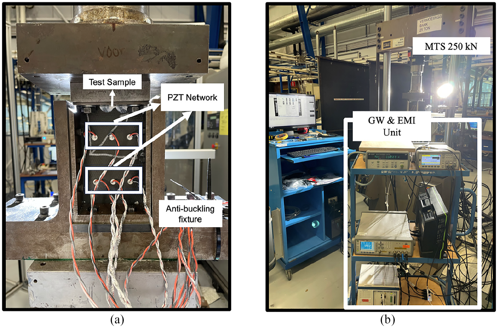
(a) PZT network attached test sample with antibuckling fixture and (b) fatigue test setup.
The sensor network used for GW and EMI applications has six PZT transducers that are linearly distributed at the top and bottom sections of the sample. PIC255 type PZT disk transducers have been used in this experiment with a diameter of 8 mm, thickness 0.5 mm, with diameter and thickness frequency constants Np and Nt; 2000 and 1420, respectively, where further information can be found in Ref. 38.
Before initiating the fatigue testing, three impacted samples were tested under quasi-static (QS) compression to determine the fatigue loading parameters. The fatigue force has been aimed at 75% of the maximum QS stress. However, the variations in impact damages, in terms of their severity, affect the maximum load level for each sample. Eventually, this fact causes a variation in maximum load values, and thus, the applied load levels have been adjusted according to the impact damage severity. Data collection steps during the fatigue testing are implemented after each QS and cyclic loading by holding the
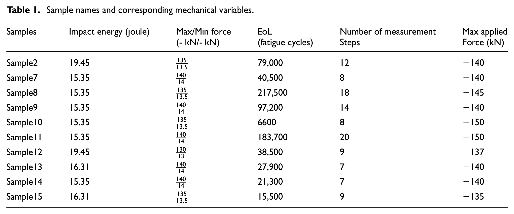
In the dataset, constant load has been applied to five samples: Samples 2, 7, 9, 13, 14, and 15. Sample 8 and Sample 11 have also been fatigued under constant amplitude load, and then the applied force is increased incrementally at the later cycles to investigate the gradually growing delamination. With a similar approach, Sample 2 is also subjected to constant loading except for its first loading cycle, in which the applied maximum load was higher than the defined fatigue force. That being the case, constant and nonconstant fatigue conditions were able to be tested. The complete data related to mechanical testing are presented in Table 1. The impact energy is considered as initial potential energy of the system, and it is calculated using Equation (1) while mg represents the total weight of the tip and attached masses, and h is the distance from the sample’s surface to the impact tip. Figure 2 illustrates the impact testing setup used to induce initial impact damage in each sample.

Sample names and corresponding mechanical variables.
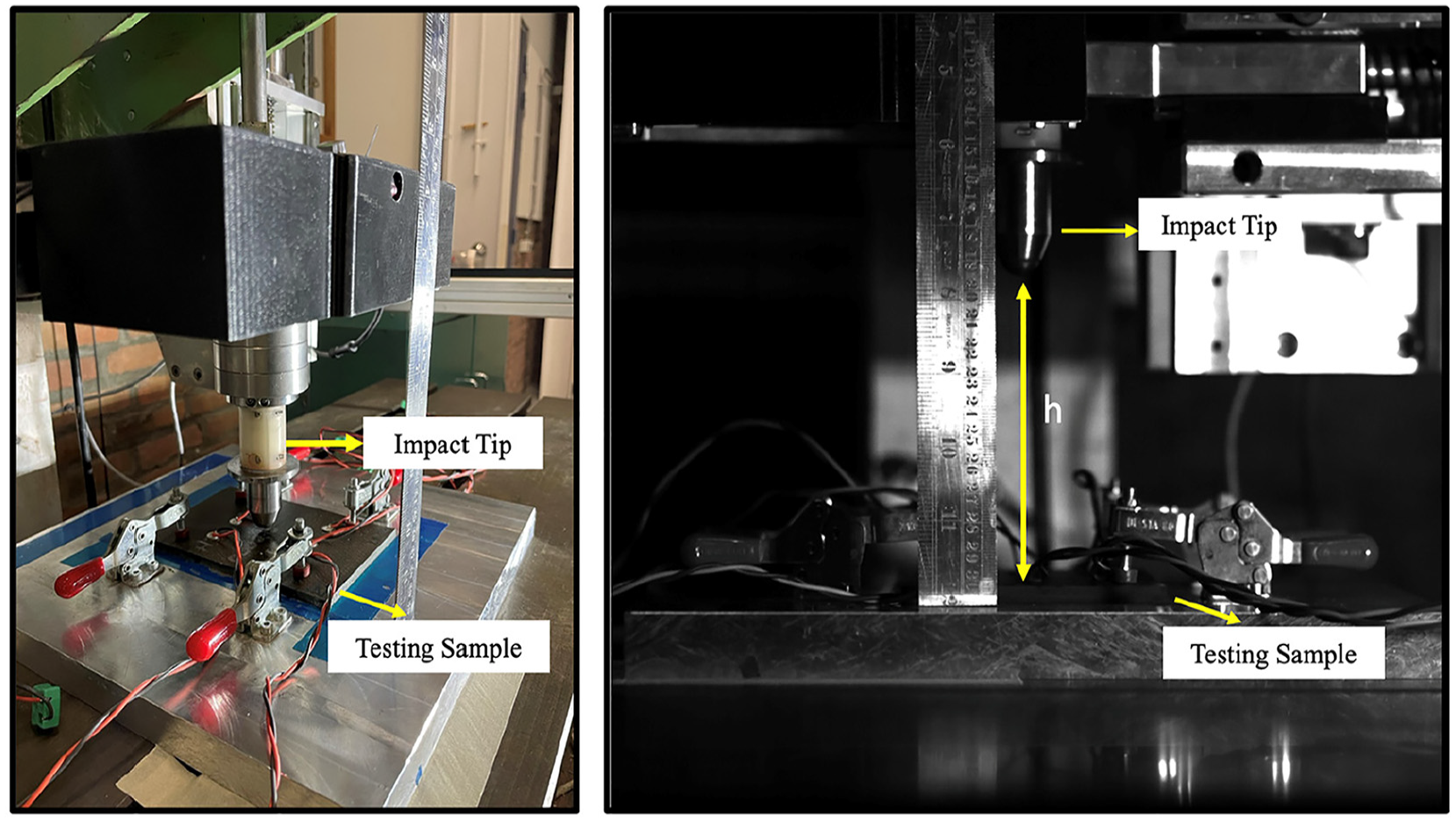
Impact testing setup (left) and impact energy calculation parameters (right).
Delamination state quantification
During the tests, ultrasonic C-scans are performed utilizing a Dolphicam 2, which operates with the pulse-echo principle at a center frequency of excitation of 8 MHz, allowing the delamination image reconstruction with postprocessing in two ways; one is with amplitude variation, and the other with time-of-flight information that enables obtaining the delamination image through the thickness. A low-pass filter is applied to the C-scan images as a postprocessing step. The obtained images are presented in Figure 3 for samples 2, 7, 9, 10, 14, and 15, as the delamination growth was present and could be captured via C-scan measurement. The initial damage states of Samples 8 and 11 demonstrated no measurable variation, which may be considered as they remained under the critical fatigue load limit or could be considered as an accumulation phase. Samples 12 and 13 are other two samples not listed in the c-scan results because of the high-noise effect in the images; thus, a linear growth regime is considered for samples 12–13. In C-scan images, the darkest blue color represents the last layer through the thickness. Delamination’s shape varied in each sample, and its propagation acceleration differed at each layer. It should be noted that the first ∼1 mm thickness of each sample is neglected to reduce the noise originated due to the reflection between the probe and the rough surface of woven samples. Despite this, it is evident in C-scan images that at the final state of delamination, called the threshold level, the deepest layer presents a noticeably higher growth rate in all the samples except Sample 10. In this study, the quantification method is chosen to be one-dimensional: the length in the direction of delamination growth manifests perpendicular to the direction of the applied load.
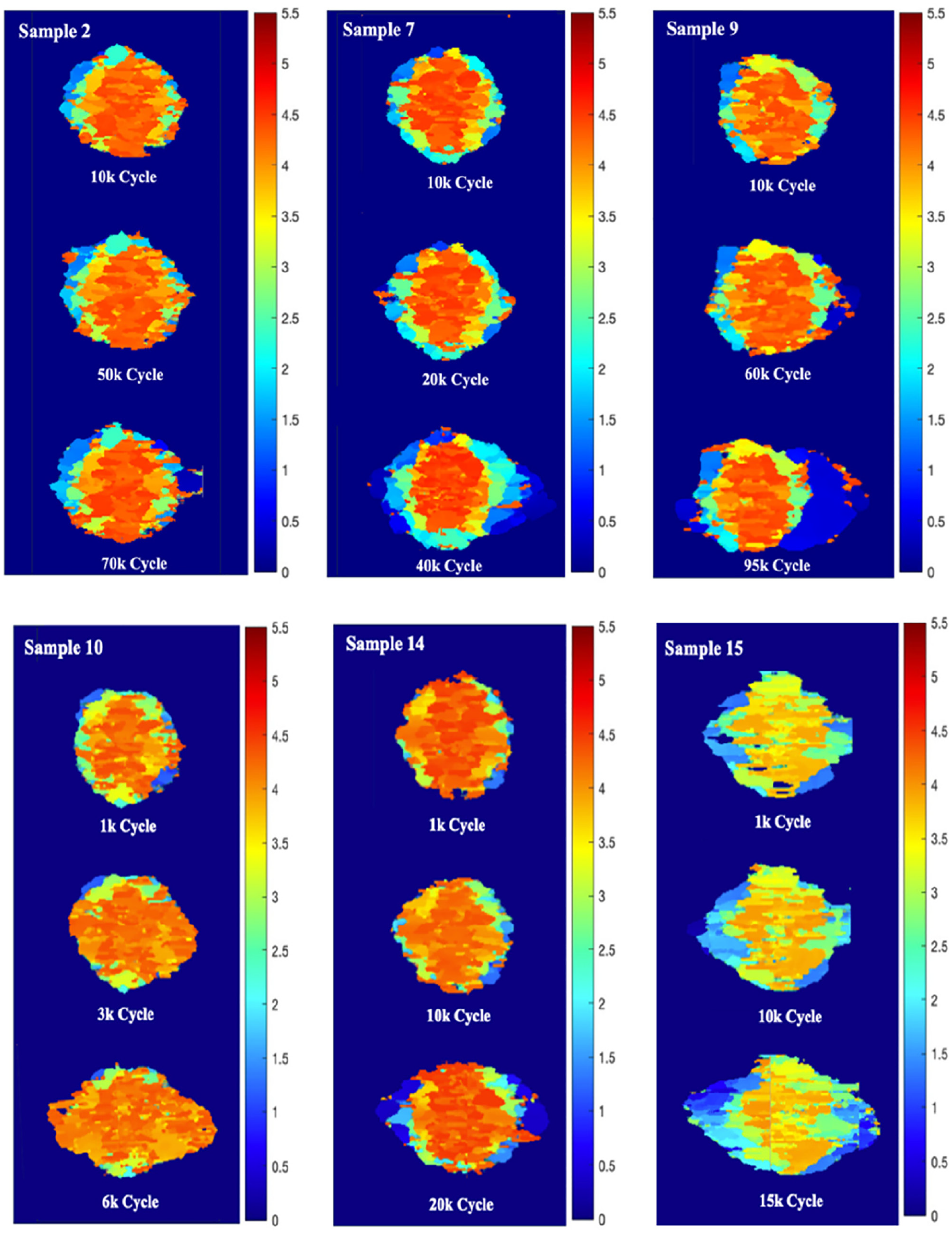
Ultrasonic C-scan images of delamination from three-fatigue life state: initial, middle, and final/threshold.
This quantification cannot involve the variations in delamination that co-occur at each layer or other types of damage, such as matrix cracks. However, maximum measured length information may help determine the evolution of the delamination during the fatigue loading. The measured delamination lengths (MDL) are indicated in Figure 4 for ten samples, where the threshold level shows the last step that allows for data collection before the failure. The maximum final delamination length is identical for all samples because it is constrained by the fixture, which is 100 mm in width. Although the EoL may occur at 100 mm, broken sensors following catastrophic failure prevent further data collection. The threshold level, which is the final state of each sample in that final measurement is taken, varies for each sample.
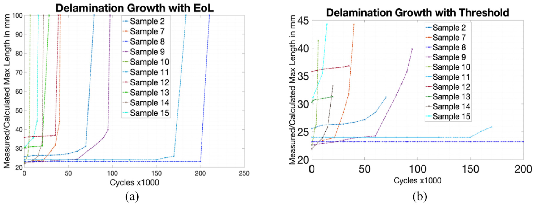
Measured delamination lengths per sample considering (a) EoL and (b) threshold.
RUL refers to the number of remaining operational times (cycles) during which the structure can perform safely. The estimation of RUL accounts for the degradation rate and the structure’s capacity to endure additional loading under operational conditions before reaching a critical threshold. This study determines RUL based on the observed delamination length, a key indicator of structural failure. This approach is depicted in Figure 5, emphasizing the connection between delamination growth and the RUL determination strategy. The increase in delamination length defines the degradation process; parameter c denotes the time interval between the threshold point and final failure, which is 2700 cycles for Sample 9.
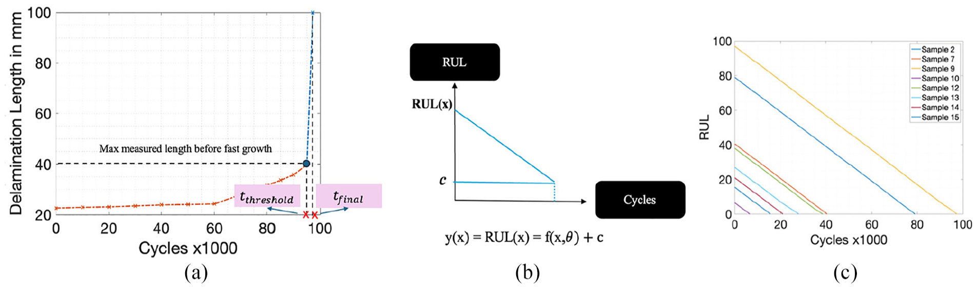
(a) Measured delamination length for Sample 9, (b) RUL definition, and (c) RUL for all samples.
SHM techniques
Methodological steps to achieve RUL prognostic based on GW-DIs and EMI-DIs, explained in this section. In the first subsection, the EMI technique will be introduced. In the second subsection, the GW method, which contains the signal processing steps for GW signals will be presented. Figure 6 illustrates the steps of the methodology contains the experimental campaign to SHM data collection that followed by signal processing, DI extraction and RUL prediction steps.
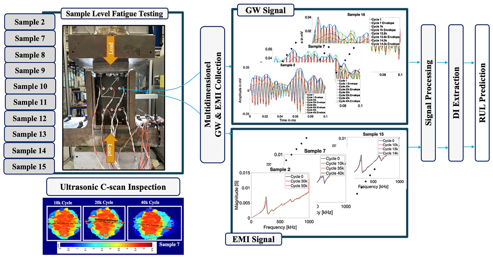
Methodological framework.
Electromechanical impedance-based damage indicator
PZT transducers are piezoelectric materials employed with the principle of transforming electrical energy into mechanical energy and vice versa, owing to the piezoelectric effect. The characteristic vibrational behavior of the structure alters as damages appear, and these vibrational variations can be measured in complex electrical admittance owing to the coupling between the PZT and the host structure. The complex electrical admittance expression is given in Equations (2) and (3) for the electromechanical admittance and the mechanical impedance of the PZT patch:
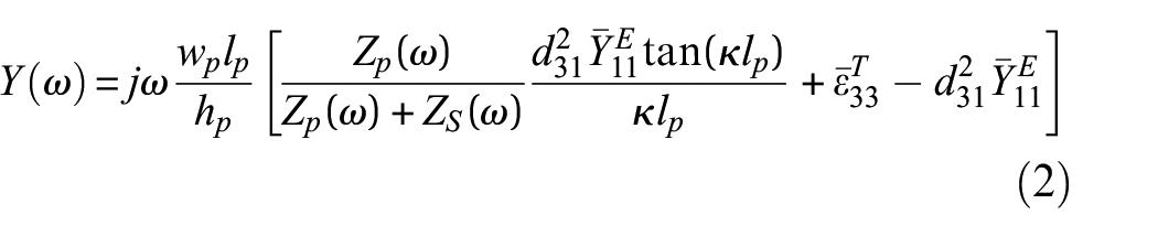
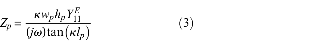
where
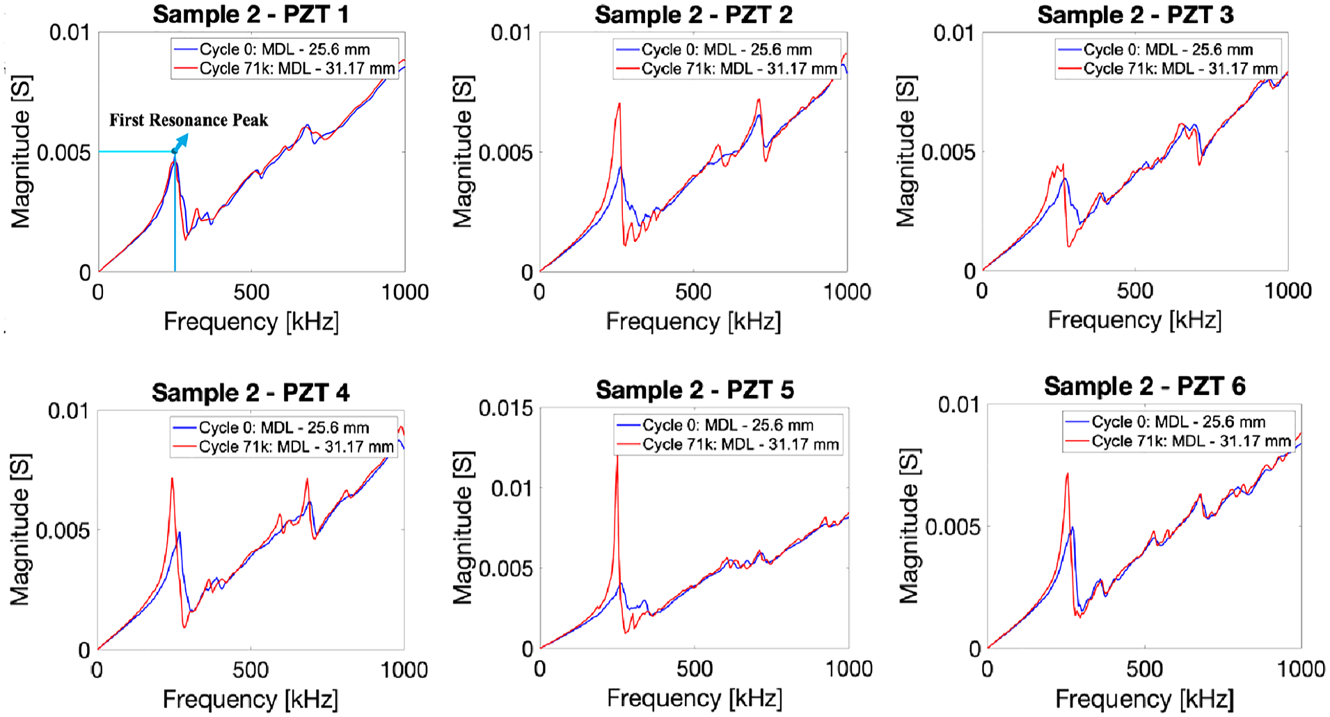
Initial and final state EMI magnitude comparison for six PZTs of Sample 2.
Guided wave-based damage indicator
GWs are a type of elastic wave that propagates in plate-like structures consisting of longitudinal and shear modes. At the same time, their characteristics are determined by the structural geometry, ply fiber direction, initial wave entry angle, and selected excitation signal and frequency. In the experiment, GW excitation signals are performed as 2-cycle tone-burst signals at the center frequency of 100, 120, 140, 160, and 180 kHz. The GW signals are acquired in the pitch-catch mode, which describes each PZT acting as an actuator and receiver step by step. While the top array PZTs are in actuator mode, only the bottom array acts as a receiver and vice versa. As a result, each PZT has three paths, and 18 paths are collected. After the preprocessing step, signal processing and DI extraction process is conducted in three main ways:
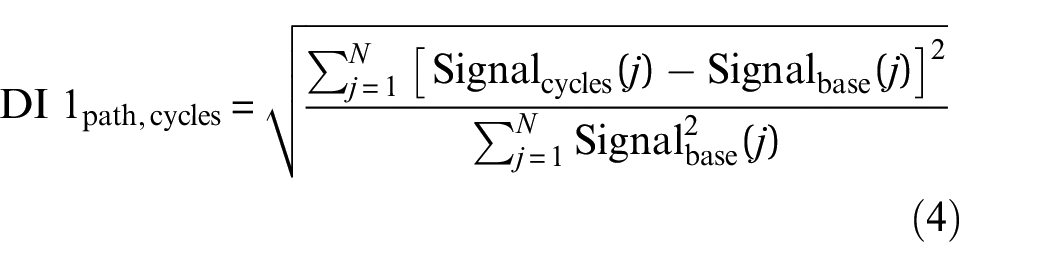
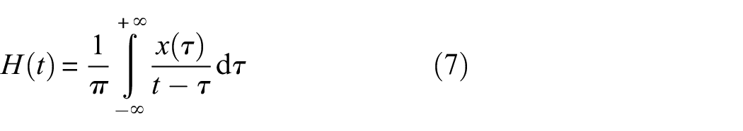
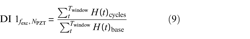
1. HT is used to obtain signal envelopes from residual GW signal that allows for the calculation of the signal energy in desired time interval given in Equation (7) to (9). A time-window is assigned with different length for each excitation signal resulting in a longer time window for a lower frequency of 100 kHz and a shorter one for 180 kHz. These intervals are 0–5; 0–4.5; 0–4; 0–3.5; 0–3.0 μs. Figure 8 shows the original and processed GW signals with envelope presentations:

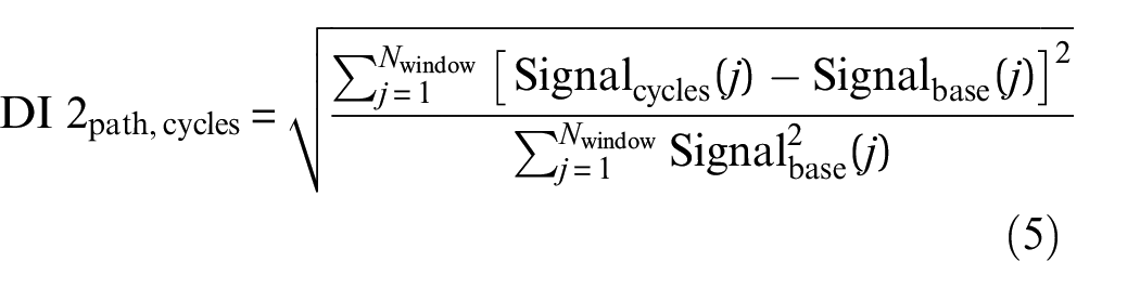
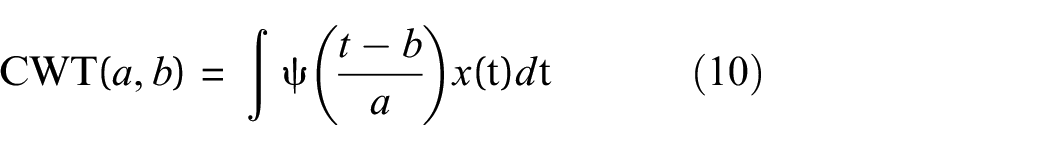
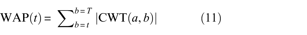
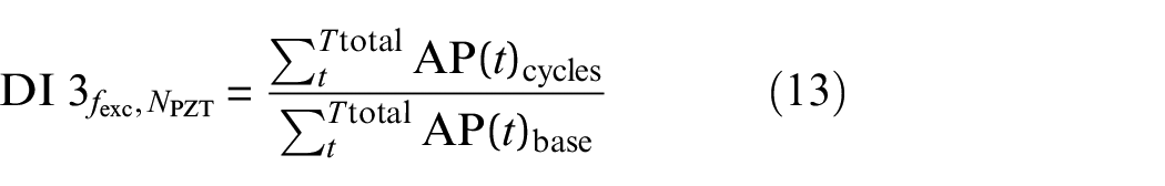
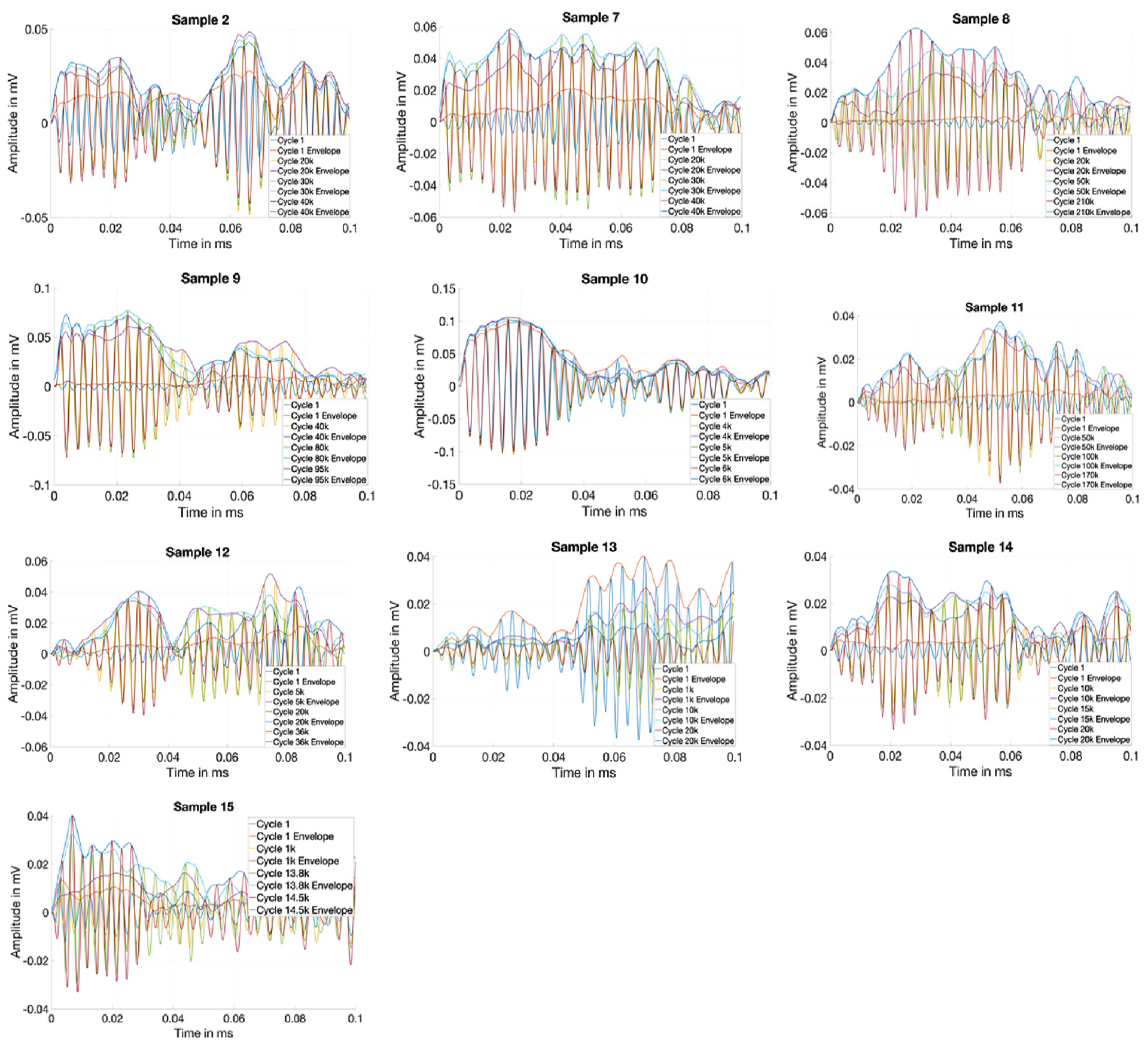
2. CWT has been applied to represent the signal in the time–frequency domain, which allows to measure energy in segments of the signal which has been achieved via windowed average power calculation where the related equations are given in Equations (10) to (13).
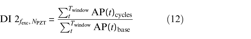
Envelope representation of GW signals between Actuator: PZT 1; Receiver: PZT 6 from 180 kHz center frequency excitation signal.
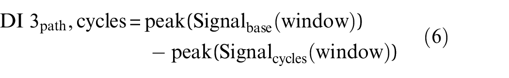
Ψ(t) is the wavelet function, and CWT(a,b) are the continuous CWT coefficients. Generally, when the signal segment shares the same form or pattern as the wavelet, the resulting wavelet coefficients achieve their maximum value. In order to detect the delamination-sensitive indicators, DI 2 and DI 3 are extracted from the average power analysis, which is derived from the time–frequency domain estimated by CWT. The time window is selected based on the final residue signal, demonstrating the higher deviation in the damage-related energy package. After determining the time scale, the total energy change is estimated in this interval to obtain DI 2. DI 3 calculates the total power change in average power analysis that accounts for all spectrums
3. The coherence of the signal all through the growing cycles is evaluated with the cross-correlation between the signals in the time domain with the following equations:
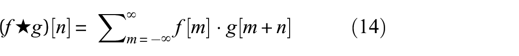
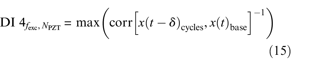
the term corr denotes the correlation coefficient function, and −δ indicates the shift of the current signal.
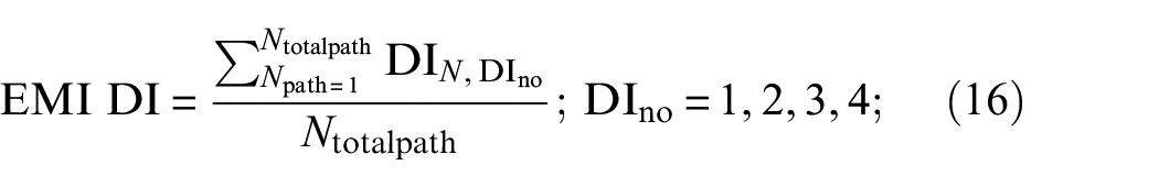
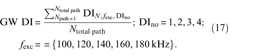
Finally, the signals from all the PZTs in the sensor network are fused with the same weight to obtain one global DI for one specific time step. Equations (16) and (17) are presents the sensor-based fusion step. In the later step, normalization with 0 to 1 range is applied for global DIs for a better representation with their corresponding MDL. On the other hand, in the prognostic stage, a sample-based standardization step is performed for fused-DIs to involve sample-based variations in the model:
Methodology
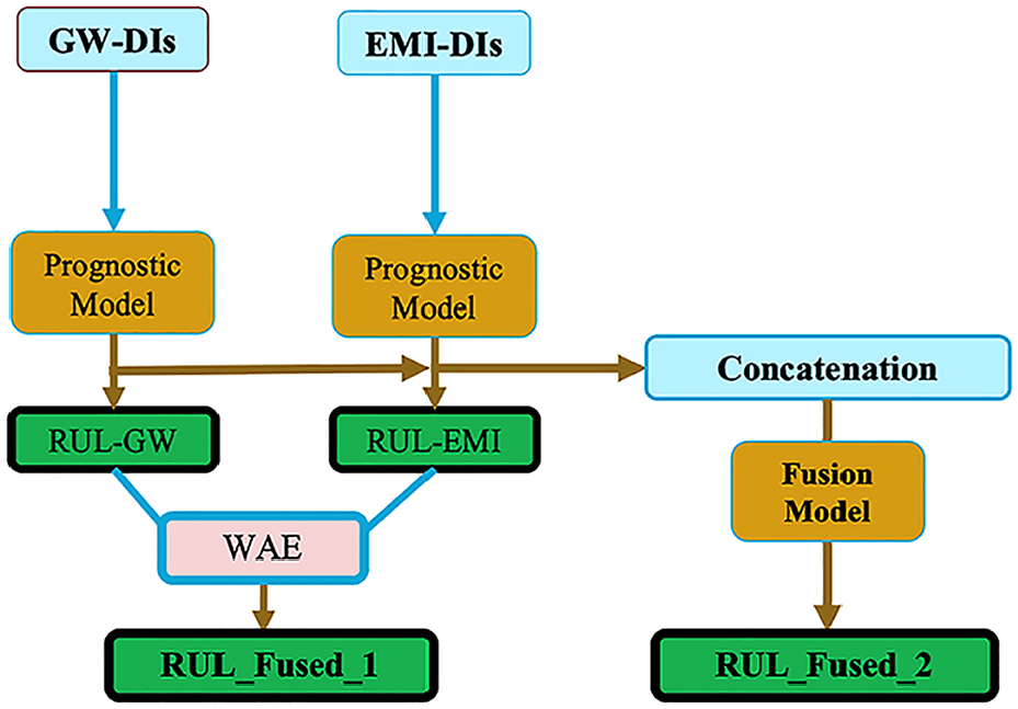
For the prognostic model, a deep neural network (DNN) model is designed as they are well-suited for tasks with high-dimensional inputs and nonlinear relationships. To explore the performance of EMI-DIs and GW-DIs, models are trained for each DI, which results in two different hyperparameter tunings for each RUL prognostic model. Two fusion methodologies are proposed for further improvement to achieve a more robust prognostic. The weighted average ensemble (WAE) considers two RUL predictions obtained each prognostic model trained via GW-DIs and EMI-DIs. The second fusion methodology concatenates the outputs of each prognostic model and then inputs them into the fusion model, which is designed as another DNN architecture with independent hyperparameter tuning and learning steps. The schematic of the proposed RUL prognostic is represented in Figure 9. The dataset was created with samples 7, 9, 12, 13, 14, and 15 by excluding samples 8 and 11 as their degradation has not been captured in terms of delamination propagation. Sample 10 is excluded because of its short EoL, which negatively affect the prognostic criteria that consider the distribution of samples’ end-of-life merit.
Schematic of the proposed fusion frameworks for RUL prognostics.
Prognostic models
DNNs have become highly effective tools for regression tasks due to their ability to model intricate relationships between input and output variables. DNNs can automatically learn hierarchical representations from data, making them particularly suitable for tasks with high-dimensional inputs and nonlinear relationships. The fundamental components of a DNN are neurons, which are arranged in layers. In a standard DNN architecture for regression, multiple hidden layers are placed between the input and output layers. Well-adapted activation functions include the rectified linear unit (ReLU), sigmoid, and hyperbolic tangent (tanh). 40 After testing various activation functions to map DI sets, ReLU was primarily utilized in the proposed model for their effectiveness in achieving higher accuracy.
Training a DNN for regression involves adjusting neuron weights and biases to minimize a loss function, which measures the difference between predicted outputs and actual labels. This is achieved using optimization algorithms such as stochastic gradient descent (SGD) or its variants, like adaptive moment estimation (Adam). 41 Adam is an adaptive optimization algorithm that maintains two moving averages of the gradients and adapts learning rates for different parameters based on their historical gradients, often leading to faster convergence and greater robustness to noisy gradients compared to traditional SGD methods. Mean squared error (MSE) is used as the loss function and accuracy metric during training and testing. The equations for Adam’s optimization strategy are provided in following:


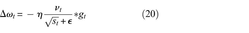

In the given equations,
Without explicit time dependence in its structure, the model is trained using input data formatted time-series. During the training phase, each iteration involves mapping an individual input value within the dataset to its corresponding RUL target. Training is conducted by sequentially feeding the model with the DI history of each sample within the training set. For testing, the model predicts RUL for each time step based on unseen data, effectively estimating RUL iteratively across the time horizon. Figure 10 presents the complete framework for RUL prognostic with the proposed learning model. Two architectures are trained for EMI-DIs and GW-DIs inputs named M-EMI and M-GW. Input sets have
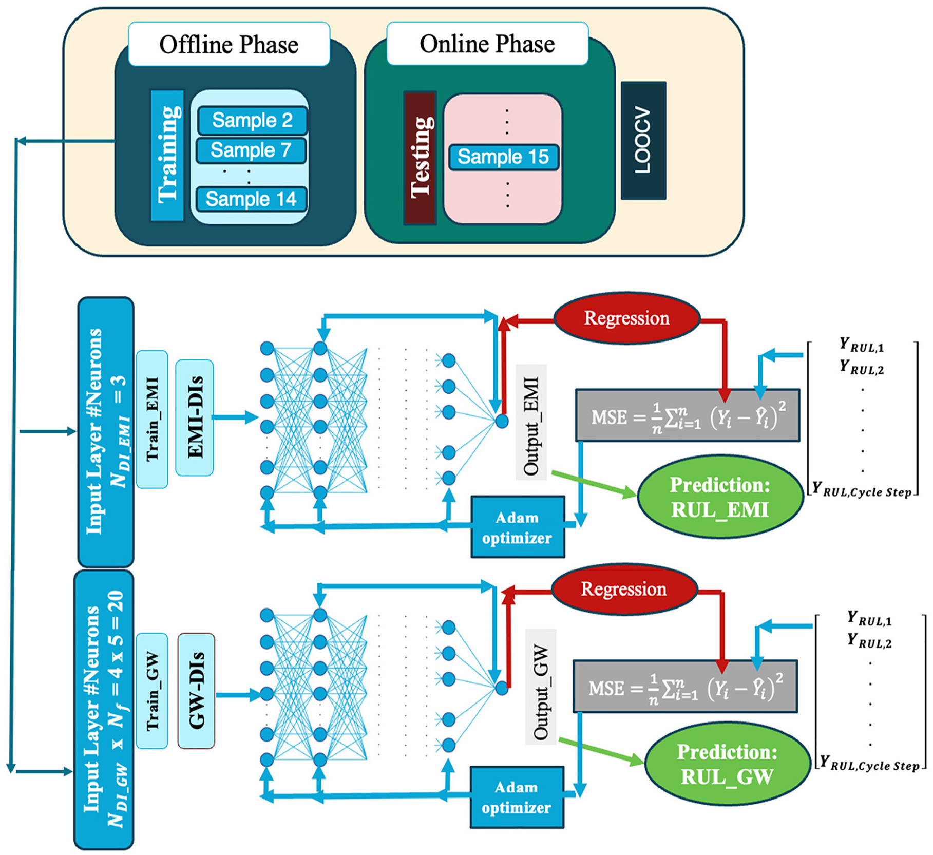
DNN scheme for RUL prognostic framework.
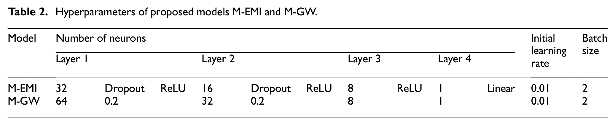
As a result, each sample was held out as a testing sample and was not included in the training phase. Finally, RUL predictions of seven samples are obtained. To account for potential missing data steps and maintain consistency, interpolation is applied to keep intervals constant. The inputs are standardized using z-score normalization applied on each DI set separately and then fed into the M-EMI model through a 3-neuron input layer. In contrast, the M-GW model utilizes a 20-neuron input layer. Hyperparameters are optimized experimentally by monitoring the training loss, which is measured as the MSE value, using validation data. The validation data are randomly selected from the training set, with 20% of the training dataset aside for validation. The solution space for the given architecture is considered to be sufficiently converged, meaning that minor adjustments in the number of neurons do not significantly impact the model’s accuracy. This suggests that the architecture is robust to small network configuration changes, indicating that the model’s performance has reached an optimal or near-optimal state within the specified design parameters. The model utilizes a batch size of 2, meaning that the parameters are updated based on the loss function after processing each pair of consecutive time steps. Final hyperparameters are given in Table 2. Dropout regularization layers 42 are applied after the first and second layers. To generate confidence bounds for the predictions, the model was re-initialized and re-trained ten times with random initial weights and biases, resulting in varied predictions each time. This approach demonstrated the stability of the proposed model by showing that predictions consistently fell within a specific range, confirming the model’s robustness across different random initializations.
Hyperparameters of proposed models M-EMI and M-GW.
Fusion methodology
As can be seen in Figure 11, two fusion approaches are proposed: WAE and DNN-fusion. WAE, shown as Fusion 1, is defined as follows:
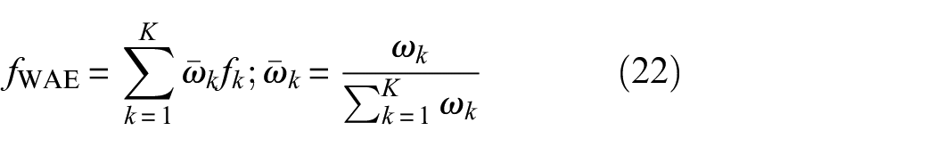
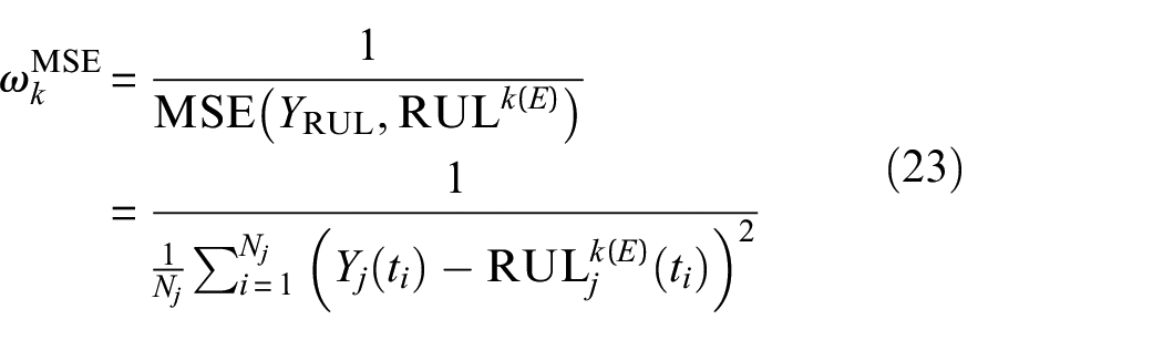
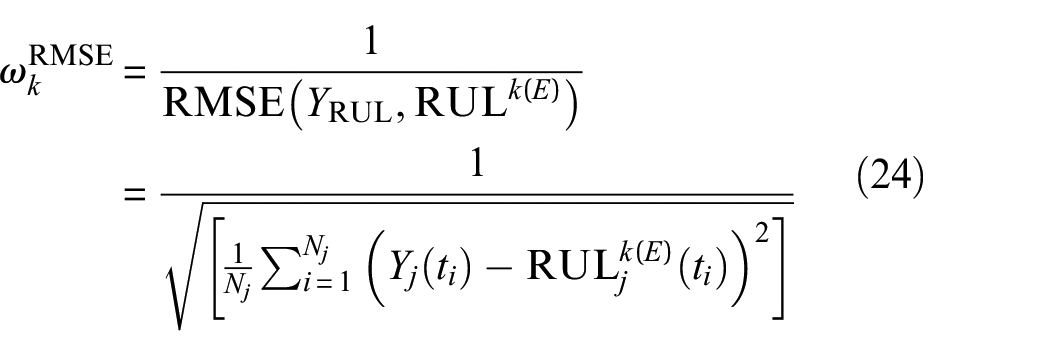
where
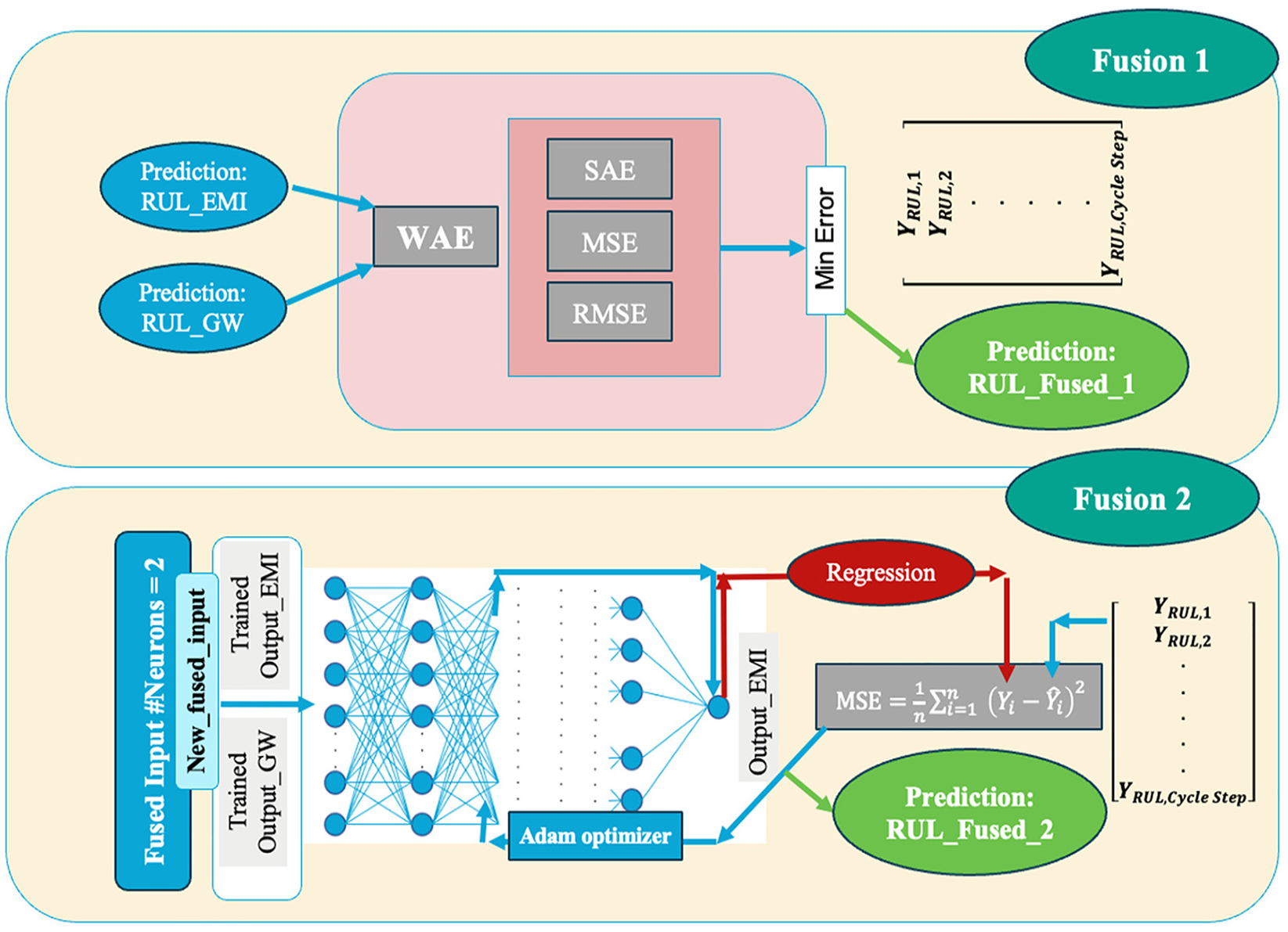
Proposed fusion methodologies to integrate RUL predictions obtained from both EMI-based and GW-based prognostic models. Fusion 1 represents the weighted average ensemble (WAE), and Fusion 2 has a deep learning basis.
RUL-fused-2 is obtained in the methodology shown in Figure 11 as Fusion 2. A DNN model is constructed to take the outputs of the GW-based and EMI-based prognostic models as inputs, and it is trained to predict the target values,
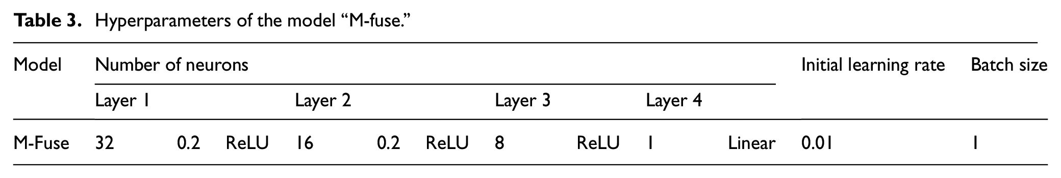
Hyperparameters of the model “M-fuse.”
Results and discussion
Damage indicators
EMI-DIs are presented in Figure 12, and their accuracy to capture delamination growth behavior is shown. In the figures, each normalized-DI is represented with its corresponding normalized-MDL. It can be seen from the results that proposed DIs are not indicating the same behavior, yet in cases of Samples 7, 9, 10, 13, and 15, there is a continuous degradation. Sample 11 and Sample 8 show a constant state of delamination even some fluctuations exist it seems like a steady-state behavior confirms their MDL. Samples 8 and 11 MDL have a limited representation after the normalization, as the earlier stages are shown at zero level. Note that no quantifiable change occurred during this period, yet impact damage exists as all the samples in the dataset. In addition to that, the load increased incrementally for Sample 11 after the 120k cycle. Even though the change in MDL seems drastic in the normalized form, the actual case can be seen more realistically in Figure 4. As so, Samples 8 and 11 are unique cases, as there was no captured variation via c-scan until a specific cycle for these two samples; EMI-based DIs also show an accumulation, and no increasing trend is shown in their DIs.
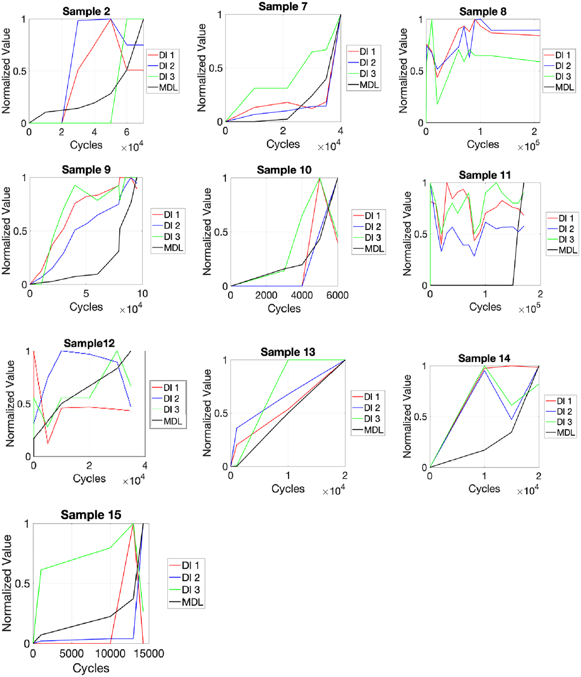
EMI-DIs and delamination growth for all samples in set.
GW-DIs are shown with the normalized MDL values for each sample in Figure 13, presenting the results for all samples from one-selected frequency that presents the highest prognostic score. As each frequency contains 4-DIs, it makes 20-DIs to investigate at the end. Therefore, most accurate results are selected and presented.
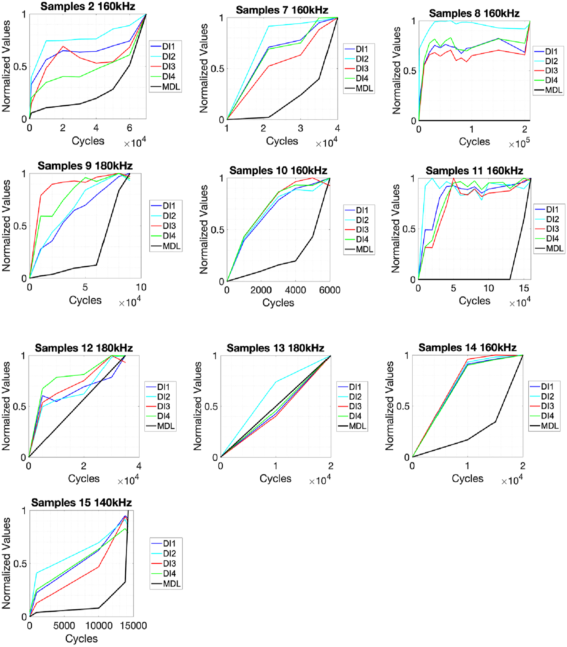
GW-DIs and delamination growth for all samples in set.
Based on the results, Samples 8 and 11 present a steady-state behavior that confirms with their EMI-DIs. Sample 8 failed in the first 7000 cycles after the 210k cycles once the load was increased with 5 kN, which did not allow for c-scan measurement before its failure. Therefore, that may prove that the increase in the severity that is observed in GW-DIs for Sample 8 may indicate the variation in the delamination even though it is not visible in MDL.
From a prognostic perspective, any DI is expected to exhibit behavior reflecting continuous structural degradation over time, given that no maintenance activities or self-healing processes take place. Thus, as damage accumulates within the structure, the associated DIs derived from GW and EMI methods should show a progressive increase. This behavior is critical for accurate RUL predictions, providing a measurable and interpretable signal of the structure’s ongoing deterioration. A monotonicity (Mo) metric is often employed to quantify this expected trend. 43 Additionally, the correlation metric can assess the similarity between DIs and observed damage degradation trends. This criterion can measure the degree to which the DIs reflect the underlying damage mechanisms as they evolve by measuring the DI correlation with measured delamination length. High correlation signifies that a DI tracks damage degradation and may enable better predictive modeling and facilitate more reliable RUL estimation. Ratings for the two metrics, Mo and Corr, range from 0 to 1, with a score of 1 denoting ideal DI performance. Considering these criteria, the following formulations for the Mo and Corr metrics are used:
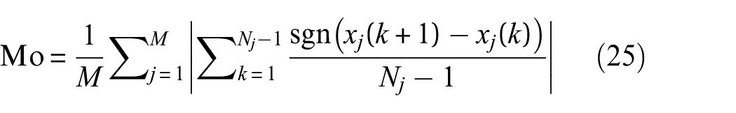
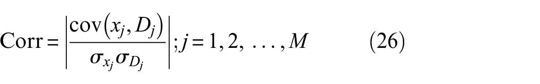
In Equation (25),
In Figure 14, the Mo performance of EMI-DIs and GW-DIs is presented for each sample. In Figure 14(a) and (b), a similar trend is observed for GW-DIs and EMI-DIs, where both monotonic and correlation metrics do not show a consistent increase or decrease across different DIs and samples. Therefore, different DI types are treated as independent features in the learning model. This strategy ensures that the learning model fully utilizes the available data, enhancing the accuracy and robustness of the prognostic methodology. In addition, GW-DIs across frequencies are treated as a single independent feature in the learning model, as their corresponding DIs do not consistently indicate the best result for a specific excitation frequency.
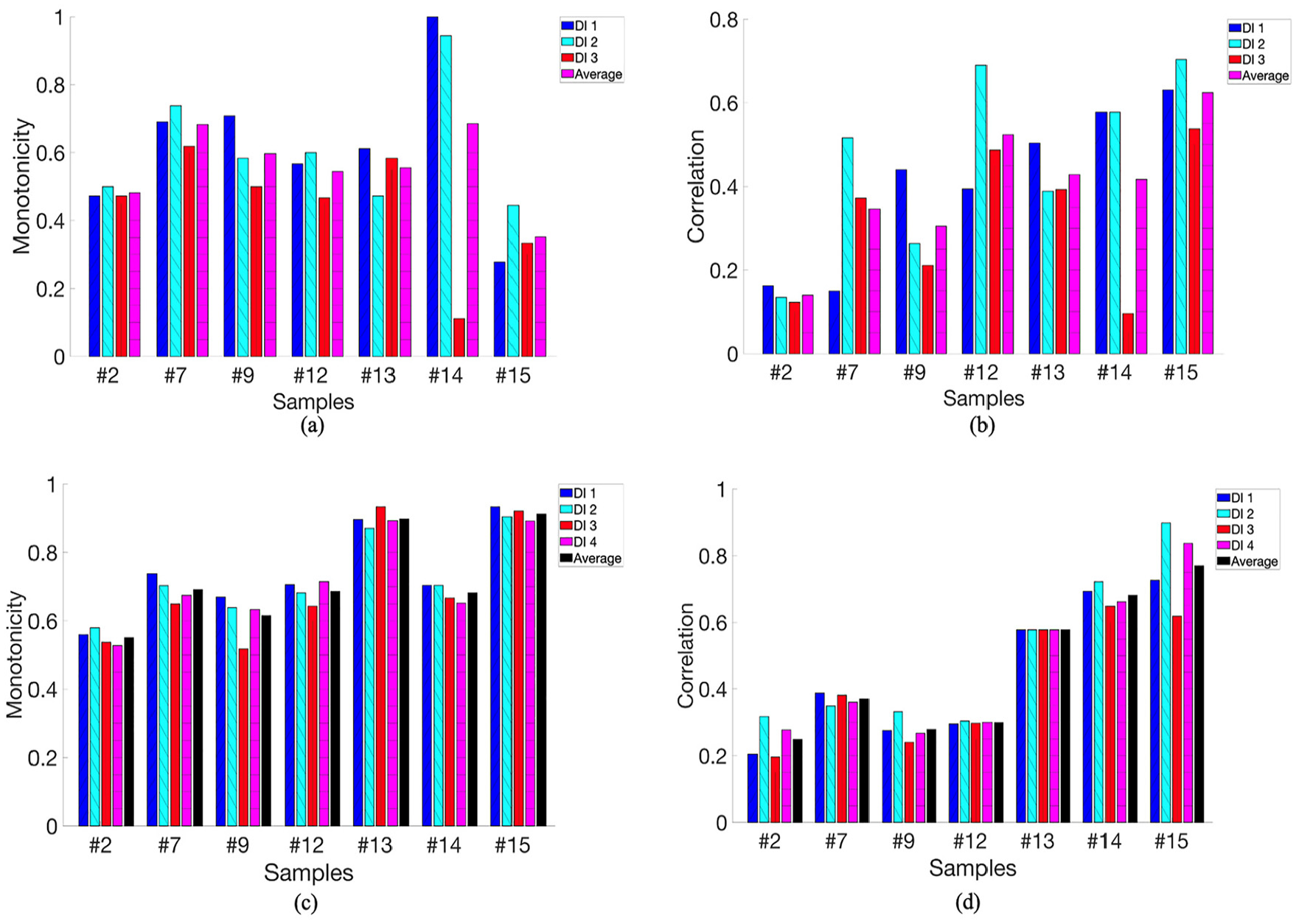
Monotonicity metric for (a) EMI-DIs and (c) GW-DIs; correlation metric for (b) EMI-DIs and (d) GW-DIs.
Prediction results
RUL prediction results are obtained as RUL-GW, RUL-EMI, RUL-fused-1 WAE-based Fusion 1, and RUL-fused-2; DNN-based Fusion 2. Errors of predictions are given by the metric of mean absolute percentage error (MAPE), given in Equation (27):
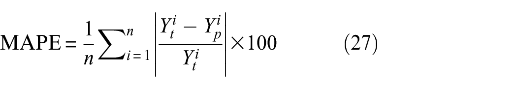
where
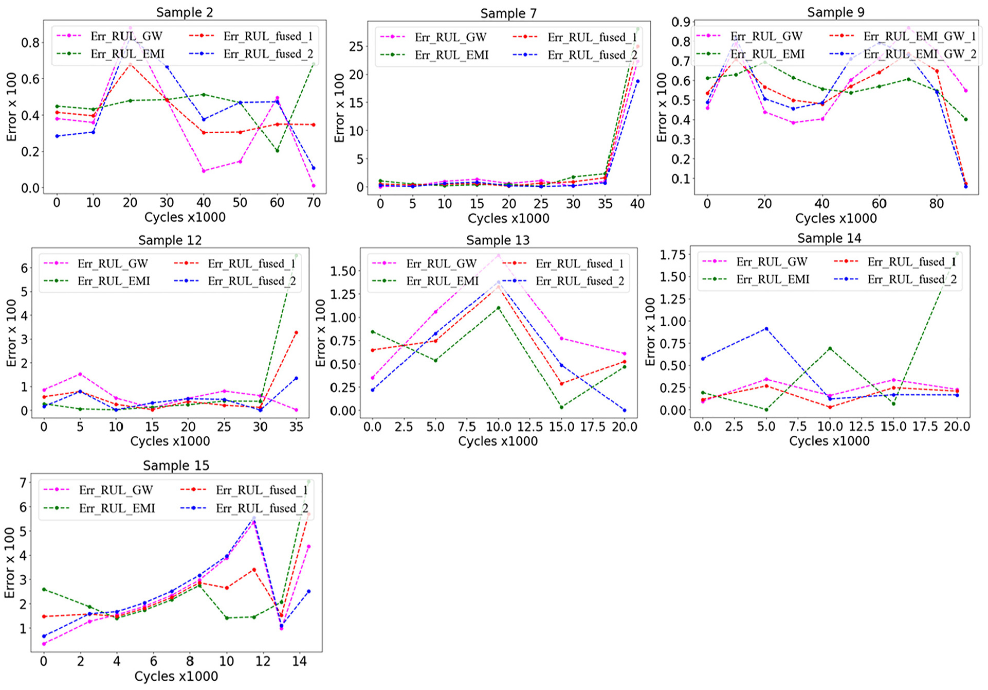
RUL results are presented in Figure 15 for seven tested samples that compare the accuracy of each input type. Among all tested samples, samples 7, 12, and 14 have the highest accuracy. The results show that the RUL accuracy differs for each input type in terms of accuracy. In Figure 16, error values regarding MAPE are given, showing the error in RUL prediction for each cycle. It can be seen in the RUL prediction results that the model performed well in terms of convergence throughout the cycle steps. For sample 12, RUL-EMI dominates the other three inputs with higher accuracy through all cycles, yet the error in the last cycle step shadows the overall performance. It should be noted that sample 12 has the highest impact energy, so the initial delamination was more severe compared to the rest of the samples, which could be captured accurately via EMI. Except for sample 12, lower accuracy for RUL_EMI holds for the rest of the samples while converging with lower error in later cycles in all cases.
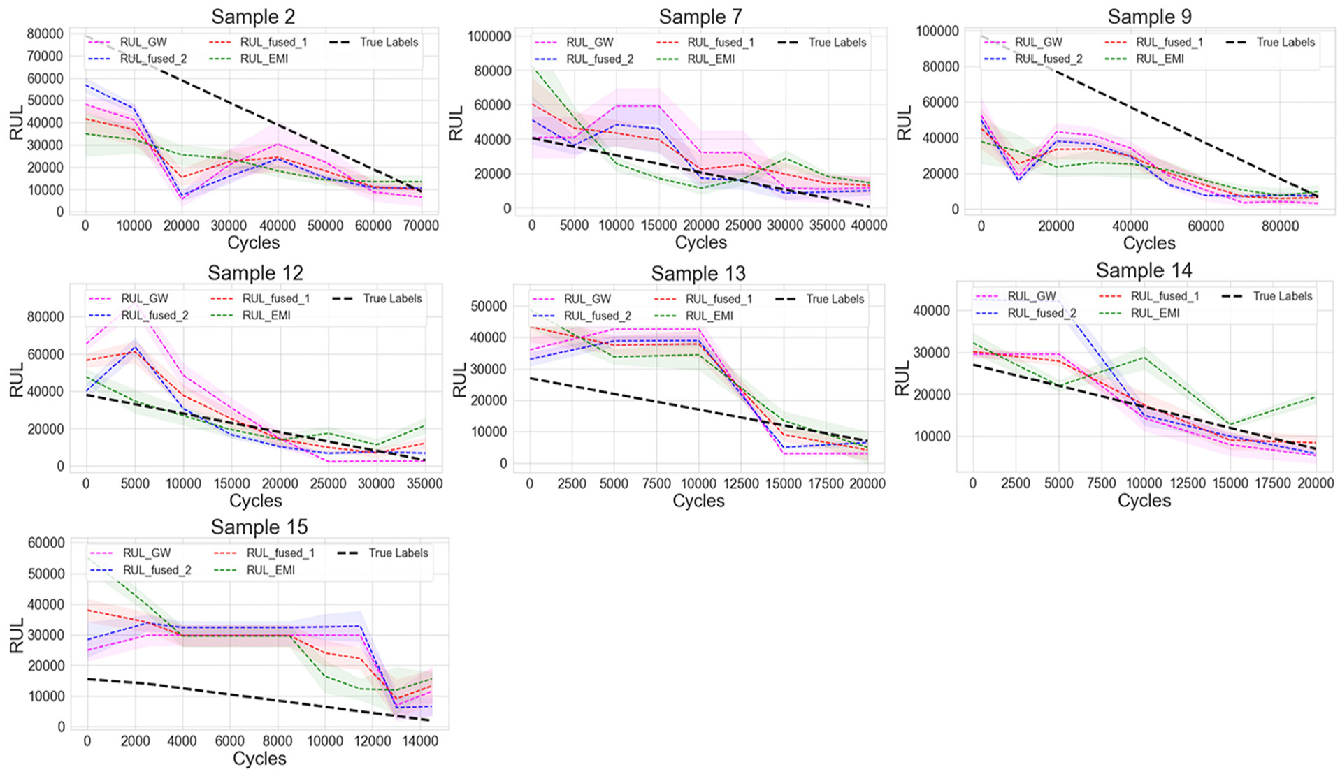
RUL predictions obtained for each model.
RUL prediction accuracy scores for each sample.
RUL-fused-1 and RUL-fused-2 demonstrate a consistent and stable performance for all tested samples. In sample 9, delamination was propagated significantly faster in one layer than in others. It is seen in its prediction that all input types perform closely, and it demonstrates an early prediction with a convergence in its final cycle. In Figure 17, the average error values for each sample are presented, and EMI_RUL has the maximum error in most of the cases. The results show that in Figure 18, while the RUL-GW operates with lower error than RUL-EMI, RUL-fused-1, and RUL-fused-2 have higher accuracy on average through the cycles in addition to the better convergence of RUL-fused-2 in the final cycle step.
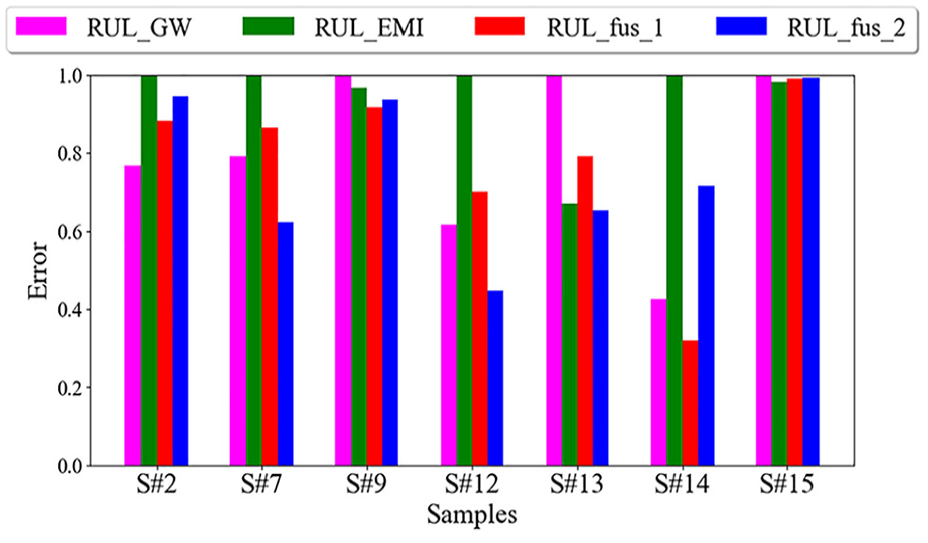
Average normalized error for each sample.
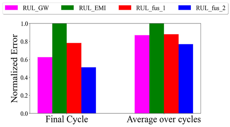
Average normalized error for each RUL model.
Discussion
To better understand the results of the obtained RUL prediction, some critical parameters need attention. Considering the load scenarios discussed earlier in this study, fast and slow growth trends in the delamination may affect the performance of GW and EMI results and the RUL prognostic. In the case of Sample 2, it is seen in the C-scan measurements that delamination presented a slow growth behavior in the earlier cycles, and it was poorly captured in EMI-DIs. It is also seen in its RUL predictions that RUL-EMI has the lowest accuracy, while RUL-GW presents significantly higher performance. That can be correlated with the fact that GW is sensitive waveforms to the slight variations in the damage and the structure. Another point regarding the performance of RUL-GW can be explained by the damage mechanisms that occur during the fatigue life of the structure and cannot be quantified through C-scan measurements. Since the GW signal conveys information from all structures and considers other damage mechanisms involved in structural degradation, GW-DIs may be more capable of predicting the RUL than EMI-DIs. However, as the delamination propagates and approaches the sensor locations, EMI performance is expected to improve, and this improvement manifests itself in RUL predictions as well.
Two different approaches were developed to integrate and leverage both techniques, with RUL_fused_2 proving to be the most robust approach, achieving higher performance in terms of final cycle convergence and throughout the fatigue life of the samples. The improvement of RUL_fused_2 is calculated considering less effective prediction of EMI and a 48% improvement in final cycle and 24% in overall cycles are achieved.
Additionally, there are some limitations regarding the proposed framework. First, the DNN model is trained via DIs obtained through signal processing. This poses a significant challenge considering the complex relation between the damage and GW signals and the limited capability of EMI measurements. Any noise or variations in the signal acquisition and processing may manifest itself in obtained DIs and can be the source of error in the predictions. Furthermore, the prognostic framework has limited degradation scenarios regarding loads and impact. Besides, proposed DNN models can be adapted to capture DIs separately from each path instead of globally represented DIs by converting them to a more complex model in terms of architecture. Finally, although the proposed prognostic methodology utilizes a DNN, there is potential to develop further and explore various regression models to more effectively leverage their respective advantages.
Conclusion and future work
This study proposed a novel framework that integrates GW and EMI signals for RUL prognostic of woven CFRP samples subject to compressive fatigue loading with impact-induced delamination. Unique characteristics of both techniques improve the reliability of the results, as the integrated methodology allows for detailed understanding by capturing the variations in DIs for different loading cases, such as fast growth and slow growth delamination effects.
A series of experiments have been carried out, including low-velocity impact, quasistatic, and fatigue testing combined with EMI and GW-based SHM applications. Surface-attached PZT networks provide the EMI and GW data, while the delamination progression is labeled with periodic ultrasonic C-scan measurements. EMI-DIs are defined based on three DIs, while four GW-DIs are obtained via signal processing. In the case of delamination presenting stable behavior during the fatigue life, EMI-DIs and GW-DIs indicate a stationary response, which can be considered an indicator of their performance in terms of their capability of projecting progressive delamination. The prognostic performance of each DI is investigated in terms of their Mo and Tr, and DIs are varied in terms of their predictive performance for each sample. Therefore, to capture this variation and convey it with RUL prognostic, a DNN model was developed to fuse EMI-DIs and GW-DIs. Finally, it demonstrated that while RUL obtained via GW-DIs performs with better accuracy than EMI-DIs on average, the proposed DNN-based fusion model presents less variation throughout the fatigue cycles and holds a higher accuracy in an average of the samples compared to sole EMI or GW-based prognostic.
As the limitations are mentioned, to mitigate the potential effects that may occur in the DI extraction step, two steps can be taken: first, the paths can be assigned as independent features into the DNN model, enhancing its ability to capture a broader representation for the degradation of the structure. Second, incorporating the total signal of GW or the measurement of EMI into the DNN model may provide more comprehensive information for improved RUL estimation. Consequently, future efforts will focus on advancing the RUL methodology by integrating these insights.
Footnotes
Appendix
Declaration of conflicting interests
The author(s) declared no potential conflicts of interest with respect to the research, authorship, and/or publication of this article.
Funding
The author(s) disclosed receipt of the following financial support for the research, authorship, and/or publication of this article: This project has received funding from the European Union’s Horizon 2020 research and innovation programme under the Marie Sklodowska-Curie grant number 860104 “Guided Waves for Structural Health Monitoring.”