Sage Journals: Discover world-class research

Abstract

In this study, extensive double-blind laboratory experiments were conducted to evaluate a novel, noninvasive method for diagnosing casing integrity using electromagnetic time-domain reflectometry (EM-TDR). This method transmits a high-frequency electromagnetic pulse into the casing and records reflected signals from integrity-related impedance changes at the wellhead. The experiments included three casing sizes—7, 5.5, and 4.5 inches in diameter—with various machined features and natural corrosion to simulate casing degradation. Over 60% of the features were less than 50% of the casing thickness, and more than 65% were narrower than a 45° azimuthal angle on the casing’s outer surface. All features larger than 1 cubic inch were successfully detected using EM-TDR. For machined features smaller than 0.1 cubic inch, identification rates were 94%, 90%, and 93% for the 7-, 5.5-, and 4.5-inches casings, respectively. For features between 0.1 and 1 cubic inch, detection rates were 90%, 89%, and 83%, respectively. In the cemented segment of the 4.5-inch casing, 50% of features between 0.1 and 1 cubic inch were identified, and reflections from the cement–air interface were also observed. Among natural corrosion features, 63.5% were detected. These results indicate that the EM-TDR method can serve as a rapid screening tool to complement existing high-resolution imaging or logging methods for monitoring casing integrity.

Keywords

Double-blind laboratory experiments casing integrity diagnose electromagnetic time domain reflectometry empirical mode decomposition degradation features identification

Introduction

Subsurface wellbore is a critical component of the energy infrastructure, enabling the extraction of essential subsurface resources, including natural gas, petroleum, and geothermal energy. According to the U.S. Energy Information Administration, as of 2022, natural gas and petroleum accounted for over 40% of the U.S. total power mix, with California’s energy portfolio comprising 36.38% natural gas and 4.67% geothermal sources. Wellbore casing plays a crucial role in maintaining the operational integrity of these systems by acting as a protective barrier that isolates the wellbore from the surrounding geological strata. Ensuring the integrity of the casing is vital, as failures can lead to the uncontrolled release of hazardous fluids or gases, such as toxic brine, methane, hydrogen sulfide, and volatile organic compounds, into shallow aquifers or the atmosphere. This isolation is essential to prevent the ingress and egress of undesirable substances, thereby avoiding potential disruptions to extraction processes. Additionally, wellbores are important for subsurface energy storage, CO₂ disposal, and other applications requiring subsurface access.

Postinstallation, the casing and cement are subject to mechanical stresses from pressure variations near the well and corrosive degradation induced by fluids.^1,2 Corrosion, mechanical damage, or cement integrity issues can compromise casing integrity, reducing the operational lifespan of the well and potentially triggering expensive remediation efforts or abandonment. A comprehensive casing integrity monitoring program is vital for maximizing asset lifespan, enhancing return on investment, and ensuring the sustainable and safe operation of wellbores.

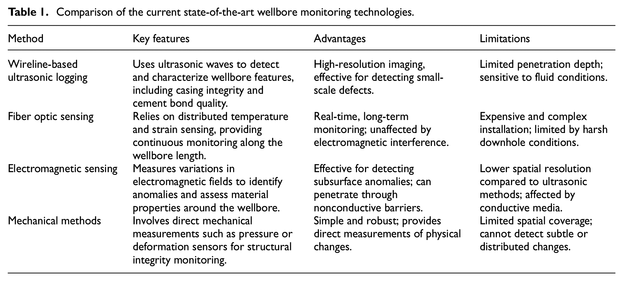
Current wellbore monitoring technologies predominantly involve downhole logging methods such as wireline-based ultrasonic logging^3,4 fiber optic sensing,^5–7 electromagnetic sensing,⁸ and mechanical methods.^1,9 A comparison of the advantages and the limitations of these methods is listed in Table 1. While these tools provide detailed insights into borehole conditions, they are inherently intrusive, disruptive to wellbore operations, or incurring significant operational costs. The extensive network of borehole facilities necessitates the development of rapid, noninvasive diagnostic techniques to supplement traditional well-logging methods, thereby reducing monitoring and maintenance expense. Presently, wellbore integrity characterization or monitoring is infrequent and often deferred until well issues become evident. Furthermore, the deployment of some of the current technologies in horizontal and high-temperature geothermal wells presents additional challenges, limiting the effectiveness of downhole tools in providing adequate data for accurate borehole degradation projections and early failure detection.²

Table 1.

Comparison of the current state-of-the-art wellbore monitoring technologies.

Method	Key features	Advantages	Limitations
Wireline-basedultrasonic logging	Uses ultrasonic waves to detect and characterize wellbore features, including casing integrity and cement bond quality.	High-resolution imaging, effective for detecting small-scale defects.	Limited penetration depth; sensitive to fluid conditions.
Fiber optic sensing	Relies on distributed temperature and strain sensing, providing continuous monitoring along the wellbore length.	Real-time, long-term monitoring; unaffected by electromagnetic interference.	Expensive and complex installation; limited by harsh downhole conditions.
Electromagnetic sensing	Measures variations in electromagnetic fields to identify anomalies and assess material properties around the wellbore.	Effective for detecting subsurface anomalies; can penetrate through nonconductive barriers.	Lower spatial resolution compared to ultrasonic methods; affected by conductive media.
Mechanical methods	Involves direct mechanical measurements such as pressure or deformation sensors for structural integrity monitoring.	Simple and robust; provides direct measurements of physical changes.	Limited spatial coverage; cannot detect subtle or distributed changes.

Nonintrusive inspection techniques, such as ultrasonic guided-wave methods, have been utilized to address these challenges.^10,11 The ultrasonic techniques leverage elastic waves generated by acoustic transducers that propagate along the pipe wall, reflecting upon encountering defects, welds, supports, or geometric changes.¹² However, this method is limited to detecting internal pipe defects and has constraints in detecting external corrosion.¹³ The resolution is limited by the low frequencies, often below 100 kHz. Additionally, casing joints impede wave transmission, further reducing the method’s effectiveness.

To address these limitations, this research explores EM-TDR as a novel approach for wellbore integrity assessment. This method, implemented at the wellhead without requiring downhole sensors, offers a nonintrusive alternative that minimizes operational disruptions and costs. Wang and Wu¹⁴ provided a proof-of-concept evaluation for the EM-TDR method’s application in wellbore characterization with preliminary field tests conducted in the Central Valley oil field. Continuing research is needed to assess the effectiveness and accuracy of EM-TDR in detecting realistic casing defects in varying degrees of corrosion and complex patterns before they reach critical failure thresholds. This study summarizes our recent progresses in evaluating the diagnostic accuracy of the EM-TDR method for a wide range of metallic casing degradation features under controlled laboratory conditions, and the development of the numerical analytical methods for signal isolation and noise reduction of the EM-TDR datasets. This study focuses on discussing the potential of EM-TDR for detecting realistically shaped casing degradation features. For this purpose, we aimed to minimize the complexity of the setup to reduce uncertainty in the analysis. While the surrounding geometrical and groundwater are important factors that affect EM-TDR signals in real-world scenarios, they are not the focus of this study.

Methods

Theoretical background

Time-domain reflectometry has been applied in locating faults on conductive cables^15,16 and in measuring soil water content and bulk soil electrical conductivity.^17–19 This technique involves sending high-frequency electromagnetic pulses into the medium under investigation and analyzing the reflected signals. Similar to the behaviors of seismic guided waves,²⁰ EM-TDR signals mainly propagate within the conductive medium being examined and reflect at interfaces with impedance changes, such as faults, damages, and terminations. In the casing integrity diagnosing scenario, the propagation of electromagnetic waves in the steel casing involves interactions between the electric and magnetic fields of the wave and the material properties of the casing. At high frequencies, the skin effect confines the current to a thin layer near the surface of the conductor, allowing the steel casing to function as a waveguide. The travel time and waveforms of the reflections (e.g., shape, polarity, and magnitude) are affected by the distances and dielectric characteristics of the impedance change (e.g., the size of the damage), respectively. Similar to the reflection seismic method, the magnitude of the reflection is mainly decided by the contrast of the impedance across the interface.

In the EM-TDR method, the voltage reflection coefficient (R) is defined as^14,21:

R = \frac{V_{r}}{V_{i}} = \frac{Z_{L} - Z_{0}}{Z_{L} + Z_{0}},

(1)

where V_r is the amplitude of the reflected voltage, V_i is the amplitude of the incident voltage, Z₀ is the characteristic impedance of the casing before the damage, Z_L is the characteristic impedance of the damaged section on the casing. As such, when the casing is either completely broken or at its end, Z_L = ∞, resulting in the reflection coefficient being 1. Conversely, when there is no contrast, such as two intact casing sections joined together, then Z_L = Z₀, and the resulting reflection coefficient equals 0. If the casing section under examination is almost perfect conductor, similar to shorted connection, then Z_L = 0. As a result, the reflection has the negative polarity, that is, R = −1. For the majority of characteristic impedance changes on the casing, the voltage reflection coefficient falls within the range of −1 to 1.

Equation (1) indicates that the reflected EM-TDR signal is determined by the characteristic impedance change along the casing. Increased metallic loss on the casing results in a larger characteristic impedance change, leading to larger reflections. Conversely, if there are no metallic losses on the casing, there will be no characteristic impedance changes and, thus, no reflections. The goal is to use the EM-TDR response to identify these changes on the casing and detect integrity issues before the pipe undergoes critical stress and reaches bursting pressure.

Data acquisition setup

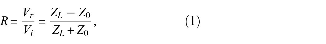
A schematic diagram of the acquisition setup is depicted in Figure 1. For EM-TDR data acquisition, source electromagnetic waves, generated from an arbitrary waveform generator, are injected into the wellbore casing through the inner conductor of a coaxial cable. The reflected signals are captured by an oscilloscope via the inner conductor of another coaxial cable. In order to minimize interference and maximize the signal clarity, the outer shield of both coaxial cables are connected to a separate coated cable suspended from top of the well and connected to the ground on the bottom of the testing facility. The coated cable provides a stable reference and ensures that the return current path is isolated. This configuration is a quasi-coaxial cable setting. A detailed theoretical analysis of the wellbore integrity application was done by Wang and Wu.¹⁴ Synchronization of the acquisition start time and the recording of the source wavelet for subsequent cross-correlation is achieved through a separate channel on the waveform generator, which sends signals directly to the oscilloscope. This direct propagation path is represented by the yellow path in Figure 1.

Figure 1.

Schematic diagram of the EM-TDR measurement setup. The coaxial cables near the casing are enlarged for clearer visualization. The yellow and blue circles indicate the two channels on both the waveform generator and oscilloscope. The red line indicates the signal-inputting route. The blue line indicates the signal-receiving route. The yellow line indicates the direction connection between the waveform generator and the oscilloscope. The green lines indicate the outer shield connected to the coated ground cable hand inside the casing.

Similar to reflection seismology, we used single pulses or short bursts as the source waveform, rather than continuous waves. Due to the limitations of our waveform generator, the highest frequency we could use was 2 GHz. Our waveform generator can only generate sinusoidal waves at frequencies higher than 770 MHz and square waves at frequencies higher than 150 MHz. In this study, when using frequencies higher than 770 MHz, the raw source waveform was a short burst of sinusoidal waves containing five cycles. When using frequencies equal to or lower than 770 MHz, the raw source waveform was a single pulse square wave. Due to this limitation, we cross-correlated the source wavelet with the raw data to ensure consistency in the acquired data. After cross-correlation, regardless of the raw source waveform, the reflected waveform appears as an impulse waveform. To mitigate reflections from the entry point of the pipe, caused by sharp impedance contrasts, a variable resistor may be incorporated into the input cable for impedance matching. While this resistor can reduce interference from impedance jumps between the input cable and the pipe, it also attenuates the input energy, particularly the high-frequency components of the signal. The decision to use the resistor depends on the specific applications. For very short pipes, where entry reflections might partially overlap with reflections from integrity-related impedance changes, incorporating a resistor can be beneficial.

Signal processing approach

A significant challenge in interpreting EM-TDR datasets is distinguishing integrity feature generated reflections from ambient noises. Employing the stacking method effectively reduces the impact of both ambient and electronic noise, thereby enhancing the signal-to-noise ratio. However, stacking cannot eliminate all random noises. In addition, if the integrity-related feature is small, it may have similar characteristics with the noise, such as wavelengths and amplitudes, making feature identification challenging. Consequently, frequency-based filters may inadvertently remove useful signals. Reflections from the beginning of the casing have higher-frequency components than those from deeper parts, even when the reflectors are of similar size, due to attenuation. Given the random nature of defect locations and sizes, predetermined or estimated parameters are needed for frequency-based filtering or wavelet analysis. This makes it challenging to remove noise without filtering out potentially useful signals. Additionally, during EM-TDR measurements, low-frequency coherent background noises are often recorded, rendering the EM-TDR signal nonlinear and nonstationary.

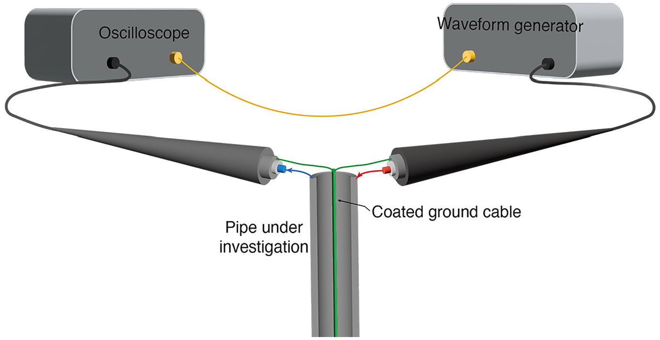
Figure 2 illustrates a synthetic EM-TDR signal to demonstrate these challenges. The synthetic casing model, 50 m in length, has three impedance features at 10, 25, and 40 m, with widths of 5, 8, and 10 cm, respectively. The impedance profile is shown in Figure 2(a). A Gaussian pulse wavelet is used as the source signal with a central frequency of 1 GHz, and the medium has an attenuation factor of 0.0002 neper/m. Figure 2(b) shows the synthetic EM-TDR signal without noise and multiple echoing reflections. Figure 2(b) shows that besides the reflections at the impedance change locations, reflections are also observed at the beginning and end of the medium. Without noise and minor attenuation, all impedance changes can be easily identified via EM-TDR reflections. To emulate a realistic scenario, we add random background noise and coherent noise at three different frequencies: 0.5, 1, and 5 kHz, to reduce the signal-to-noise ratio and introduce nonstationary elements. The synthetic noisy EM-TDR signal is shown in Figure 2(c), where true reflections are almost completely obscured by noises. Without prior knowledge about reflector sizes, locations, attenuation factors, and added noises, using frequency-based filtering methods becomes challenging.

Figure 2.

Synthetic EM-TDR data: (a) impedance model, (b) clean simulated EM-TDR signal with only attenuation effect, and (c) Simulated EM-TDR signal with both random and coherent noise. The horizontal axis is converted from travel time to distance in meter.

To address these challenges, empirical mode decomposition (EMD) was employed for signal processing to improve feature identification from noisy data. EMD, introduced by Huang et al.,²² is an adaptive decomposition technique specifically designed for nonlinear and nonstationary signals. EMD employs a sifting algorithm to adaptively decompose a given signal into a finite set of modulated components known as intrinsic mode functions (IMFs), representing the oscillation modes embedded in the data. The EMD algorithm involves the following steps²³:

In the time domain of signal x(t), find all the local extrema between two successive zero crossings.

Interpolate between all maxima and minima to generate the upper and lower envelope E_u and E_l of x(t).

Calculate the mean of the upper and lower envelopes: m = (E_u + E_l)/2.

Subtract the mean from the data: h(t) = x(t) –m, and check if the resulting data meet the IMF criteria.

If the IMF criteria is met, then subtract IMF₁(t) from original signal x(t): r₁(t) = x(t) − IMF₁(t), and repeat steps 1–4 on r₁. If not, apply steps 1–3 on h(t) iteratively until the IMF criteria is met.

IMFs should satisfy the following criteria: the number of extrema and zero crossing should be the same, and their envelope should be symmetric with respect to zero. By iteratively applying the sifting process until the residual signal, r_n(t), is monotonic, the EMD algorithm decomposes signal x(t) into IMFs and a residual:

x (t) = \sum_{i}^{n} IM F_{i} (t) + r_{n} (t)

(2)

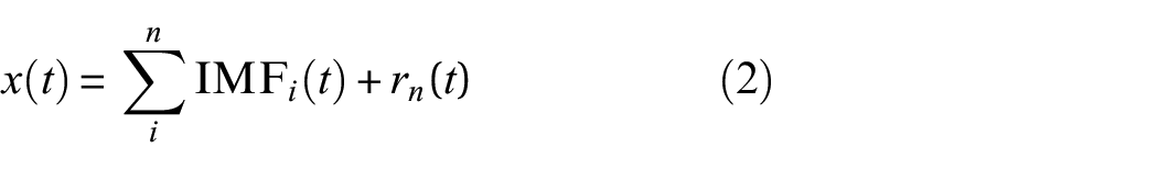
Figure 3 demonstrates an example of the sifting process applied to the synthetic data shown in Figure 2(c). For a detailed illustration, only the zoomed-in view between 10 and 12 m of the original data (Figure 2(c)) is displayed. The sifting process effectively identifies the fastest oscillation in the data (Figure 3(b)) and extracts them during each iteration (Figure 3(d)).

Figure 3.

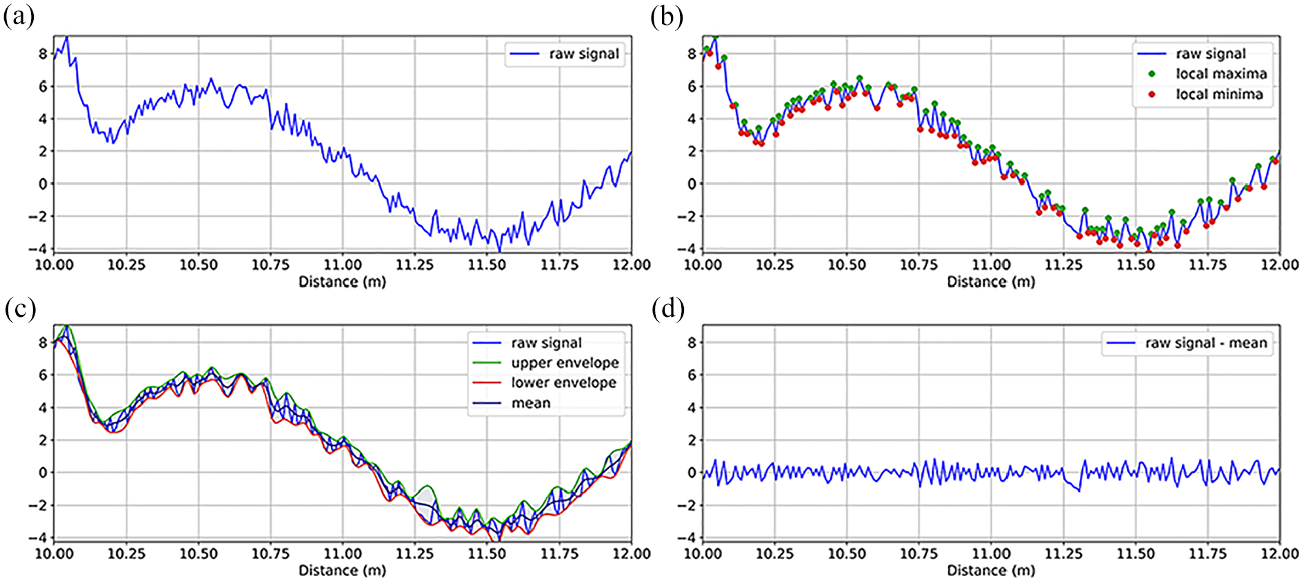
Example of sifting process during EMD: (a) zoomed in view (10–12 m) of the raw signal from Figure 2(c), (b) extracted local maxima and minima, (c) interpolated upper and lower envelopes and the mean between them, and (d) result of first iteration of sifting.

The resulting IMFs represent the inherent oscillatory modes within the original signal, providing valuable insights into its temporal dynamics and frequency characteristics. Figure 4 shows the resulting IMFs from the synthetic signal in Figure 2(c). As seen, the random and coherent noise is well separated from the signal. Comparing IMF3 (Figure 4(c)) with the clean synthetic signal (Figure 2(b)), the reflections from all impedance changes are correctly extracted.

Figure 4.

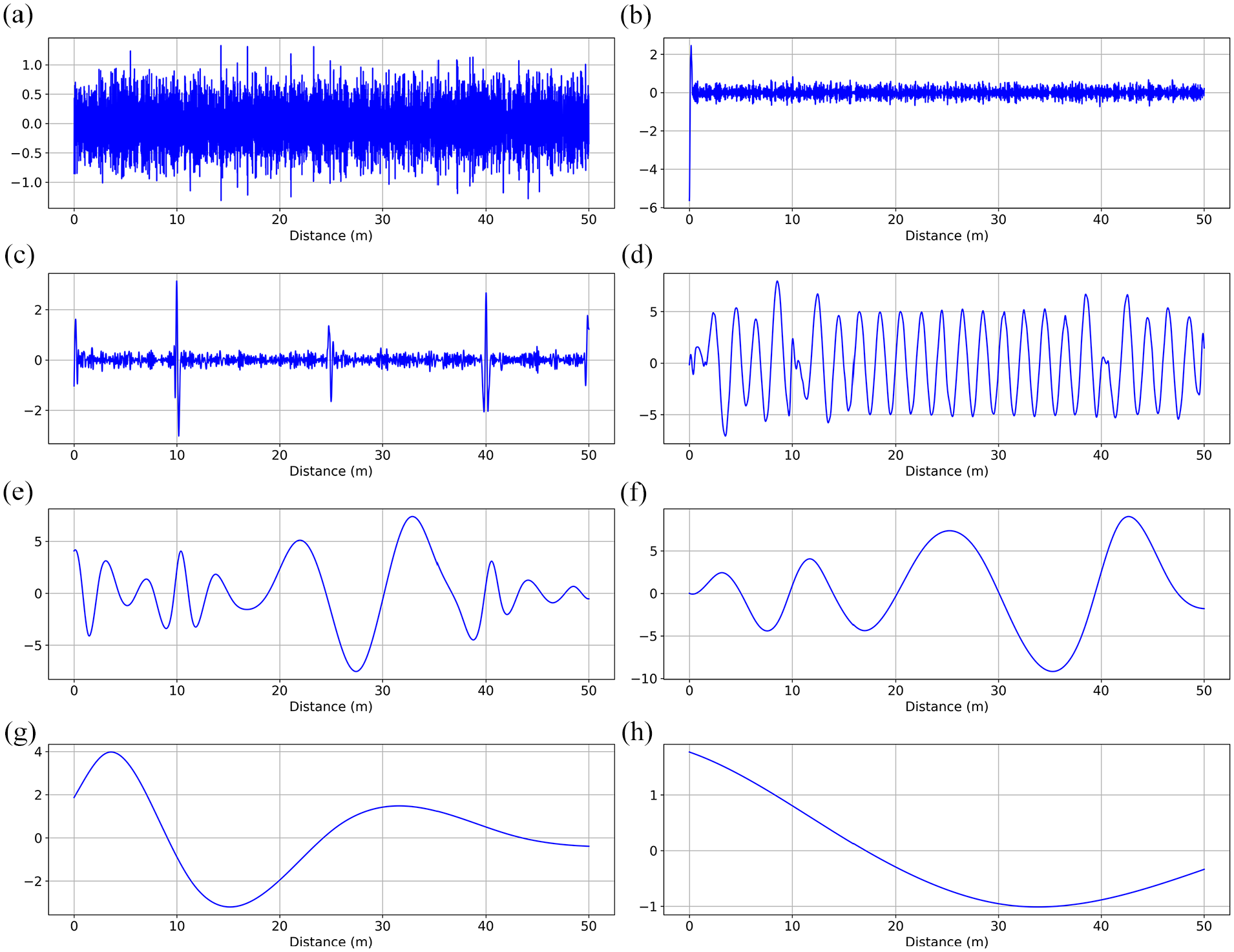
The resulting IMFs after applying EMD on the synthetic data shown in Figure 2(c): (a)–(h) represent IMF1–IMF8, where IMF3 (c) contains the feature signals.

EMD presents an alternative approach to time–frequency analysis, operating entirely within the time domain. Unlike traditional frequency-based filtering methods, which rely on predefined basis functions or filters, EMD is a data-driven process with minimal assumptions about the underlying signal, other than it being composed of different oscillatory modes. This flexibility allows EMD to be applied to a wide range of signals without extensive preprocessing or parameter tuning, which is often required for frequency domain filtering techniques. By iteratively isolating the fastest oscillations, EMD can effectively distinguish between noise and meaningful signals, particularly valuable when noise obscures important features.

After obtaining the IMFs from the EMD process, we can select IMFs of interest, exhibiting relatively low noise levels, to reconstruct the EM-TDR signal. This reconstruction aims to highlight the nonlinear and nonmonotonic components in the original signal, likely indicative of true reflections. By emphasizing these features, the reconstructed signal provides a clearer representation of the EM-TDR measurement. Due to the adaptive nature of the EMD method, which is not strictly mode-bounding, the criteria for IMF selection are determined on a case-by-case basis. In this numerical example, IMF2 and IMF3 clearly contain useful information and were therefore retained. In other cases, the IMFs selected for retention may vary.

It is worth mentioning that other signal decomposition methods can also be utilized for data analysis. A variation of EMD is variational mode decomposition (VMD).²⁴ Unlike the iterative sifting approach used in EMD, VMD is an optimization-based method that iteratively updates the modes and their center frequencies until convergence. Figure 5 presents an example of applying VMD to the same synthetic data shown in Figure 2(c). As shown, the results of VMD in Figure 5 are comparable to those obtained using EMD. However, achieving desirable results with VMD requires some degree of prior knowledge about the data for parameter tuning. In our case, the size of the features varies significantly, and attenuation alters the frequency components of reflections from these features. For our purposes, we prefer an adaptive method that does not rigidly require prior knowledge of the data for parameter tuning. Additionally, during the exploratory phase of EM-TDR development, simplicity and ease of implementation are critical. Therefore, we consider EMD to be better suited for separating noise from potentially useful signals compared to VMD.

Figure 5.

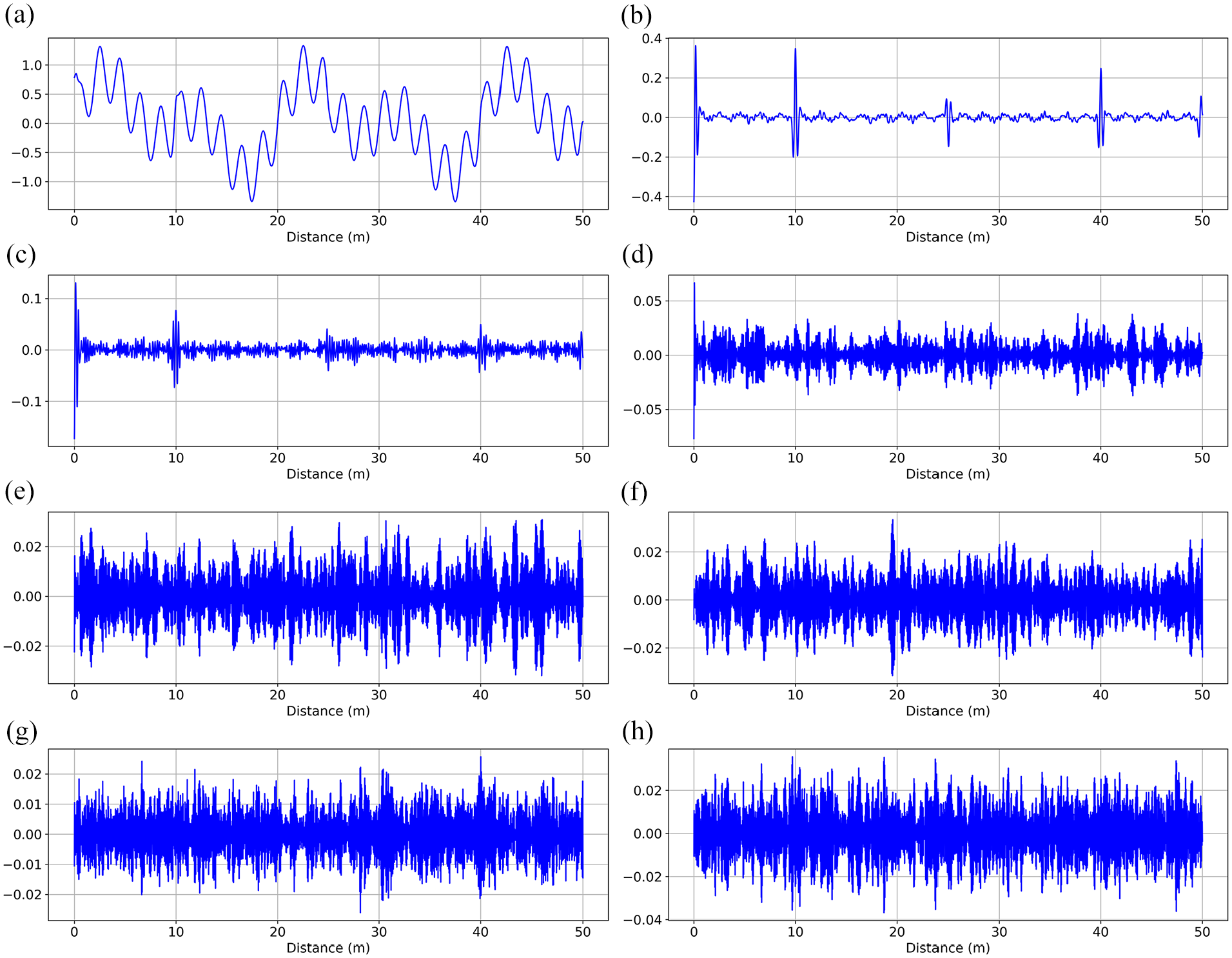
The resulting IMFs after applying VMD on the synthetic data shown in Figure 2(c). (a)–(h) represent IMF1–IMF8, where IMF3 (c) contains the feature signals.

In addition to VMD, wavelet-based methods are also commonly used for data analysis. However, these methods require the selection of an appropriate wavelet and decomposition level, and they have limited adaptability to highly nonstationary signals. For diagnosing wellbore integrity, the lack of prior knowledge and the presence of highly nonstationary signals are typical challenges. Figure 6 shows the time–frequency spectrum obtained by applying the continuous wavelet transform (CWT) to the same synthetic data presented in Figure 2(c). The Morlet wavelet was used in this analysis. Compared to the results from EMD, the resolution of the CWT is lower, indicating that it would be more challenging to detect small-scale features.

Figure 6.

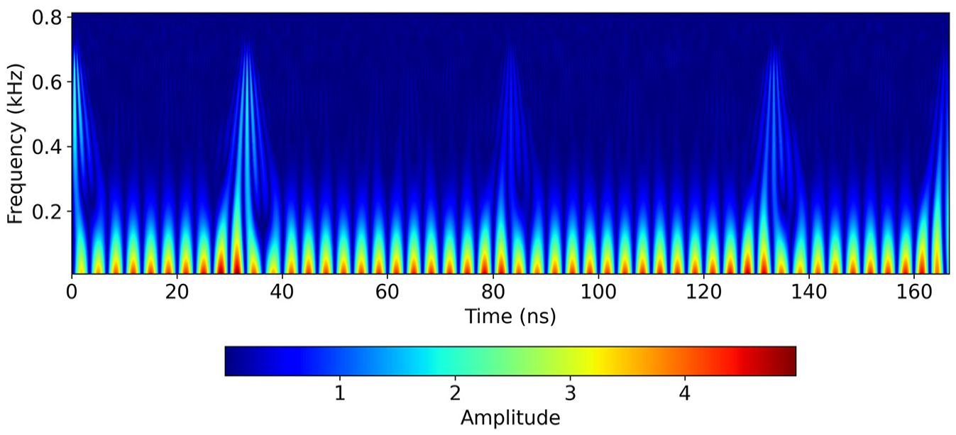
Time–frequency spectrum from applying CWT to the synthetic data shown in Figure 2(c).

Small-scale laboratory feasibility test

To evaluate the accuracy of using EM-TDR for casing integrity characterization and demonstrate the EMD signal processing method discussed above, we first conducted laboratory experiments under simplified, controlled conditions. To ensure the accurate recording of the full EM-TDR signal and correct synchronization of the triggering time, the length of the direct propagation cable was made shorter than the cable connected to the pipe. To enhance the signal-to-noise ratio, all data were stacked 300 times.

A schematic representation of the degradation feature on the pipes undergoing the test is shown in Figure 7(a). The pipes were part of the gathering pipeline, excavated from a local PG&E (Pacific Gas and Electric Company, a subsidiary of PG&E Corporation) natural gas storage facility. Each pipe had a single-machined circular pit (Figure 7(b)) to emulate the degradation. The surface diameters of the degradations were set at 0.5 inch and 1 inch, respectively. Figure 7(b) shows the top-view photographs of the machined degradation features. For each diameter, two different degradation depths were tested: 25% and 50% of the wall thickness, respectively. The machined degradations were machined with a flat drill, resulting in flat bottom and depth variations across the degradation area, with the center having the most metal loss and the edges the least. Given the small size of the machined degradations, the test frequencies were centered at 1 GHz.

Figure 7.

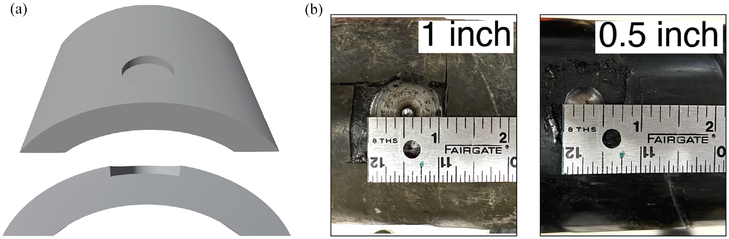
Schematic representation of the EM-TDR small-scale laboratory feasibility test: (a) schematic 3-D model of the machined feature in on the casing and (b) photographic examples of the machined features in the size of 1-inch and 0.5-inch diameter, respectively.

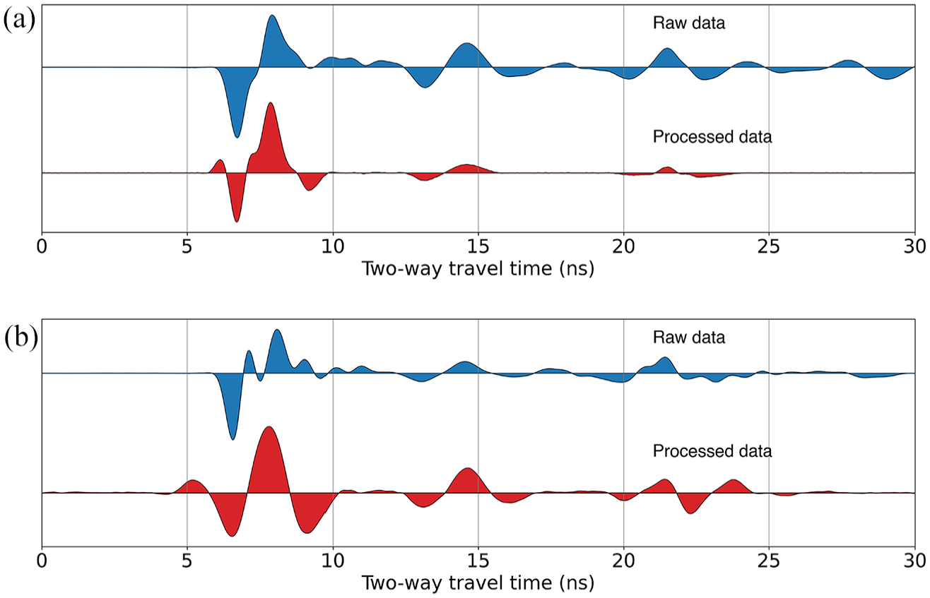
Figure 8 presents the EM-TDR test results on the pipes with 25% thickness loss features with diameters of 0.5 inch and 1 inch, respectively. The blue wiggle plots represent the raw EM-TDR data, while the red wiggle plots show the processed data. The data was cross-correlated with the source wavelet and then reconstructed using the EMD method. In the raw data, the main reflection events are visible: reflections from the beginning of the pipe (entry reflections) at around 6 ns, reflections from the machined degradations at around 16 ns, and reflections from the end of the pipe at around 22 ns. However, the waveforms of the reflections are not clean. After cross-correlation and EMD reconstruction, the reflections are clearer, and background noise is significantly reduced. Notably, in the processed data, a new set of weaker reflections becomes visible (indicated by gray boxes in Figure 8). These reflections result from double bouncing at the entry point upon the wave entering the pipe due to imperfect coupling. Specifically, the reflection from the top of the pipe bounced again inside the cable leading to the pipe, forming a closely following secondary input source. The double-bouncing reflections are relatively weak, so in the raw data, they merge with the primary reflections and form a wide complex waveform. After processing, these two input signals are well separated. In Figure 8(b), the double-bouncing wave is weaker, resulting in the double-bouncing from the end of the pipe being too weak to be seen, even in the processed signal.

Figure 8.

EM-TDR results from small-scale laboratory feasibility test on two machined featured pipes with 25% thickness loss and diameter of 0.5 inch and 1 inch, respectively. The blue wiggle plots are the raw data. The red wiggle plots are the processed data:(a) test result from the 6-feet pipe with a machined feature of 0.5-inch diameter and 25% thickness loss and (b) test result from the 6-feet pipe with a machined feature of 1-inch diameter and 25% thickness loss.

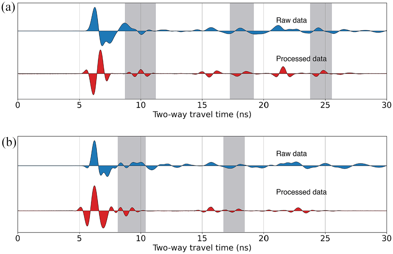
To attenuate the double-bouncing reflections, a resistor was added between the signal generator and the pipe. The resistor attenuates the input signal, but will make the double-bouncing signal even weaker. This approach was tested on two new pipes with the same diameter configuration but with 50% thickness loss. The results are shown in Figure 9. Due to the attenuation caused by the resistor, the EM-TDR signal has more low-frequency content compared to Figure 8. Similarly, the main reflections are visible in the raw data. In the processed data, the double-bouncing signal is greatly reduced, resulting in sharper reflections.

Figure 9.

EM-TDR results from small-scale laboratory feasibility test on two machined featured pipes with 50% thickness loss and diameter of 0.5 inch and 1 inch, respectively. The blue wiggle plots are the raw data. The red wiggle plots are the processed data:(a) test result from the 6-feet pipe with a machined feature of 0.5-inch diameter and 50% thickness loss and (b) test result from the 6-feet pipe with a machined feature of 1-inch diameter and 50% thickness loss.

Laboratory deep-well simulator test

Experiment set up

To further evaluate the effectiveness and accuracy of using EM-TDR for casing integrity diagnosis in a more complex scenario, we conducted more comprehensive tests at C-FER Technologies, an engineering testing lab in Alberta, Canada. The experiments utilized a Deep-Well Simulator at C-FER, capable of hosting larger diameter, vertical casings. The testing involved casing strings with three different diameters: 4.5 inches, 5.5 inches, and 7 inches. These casing strings, ranging between 80 and 90 feet in length and composed of three to four sections of varying lengths, were suspended from a ground-level supporting plate into the Deep-Well Simulator (Figure 10). To evaluate the potential impact of cement on EM-TDR performance, the bottom section of the 4.5-inch casing string was cemented (Figure 8).

Figure 10.

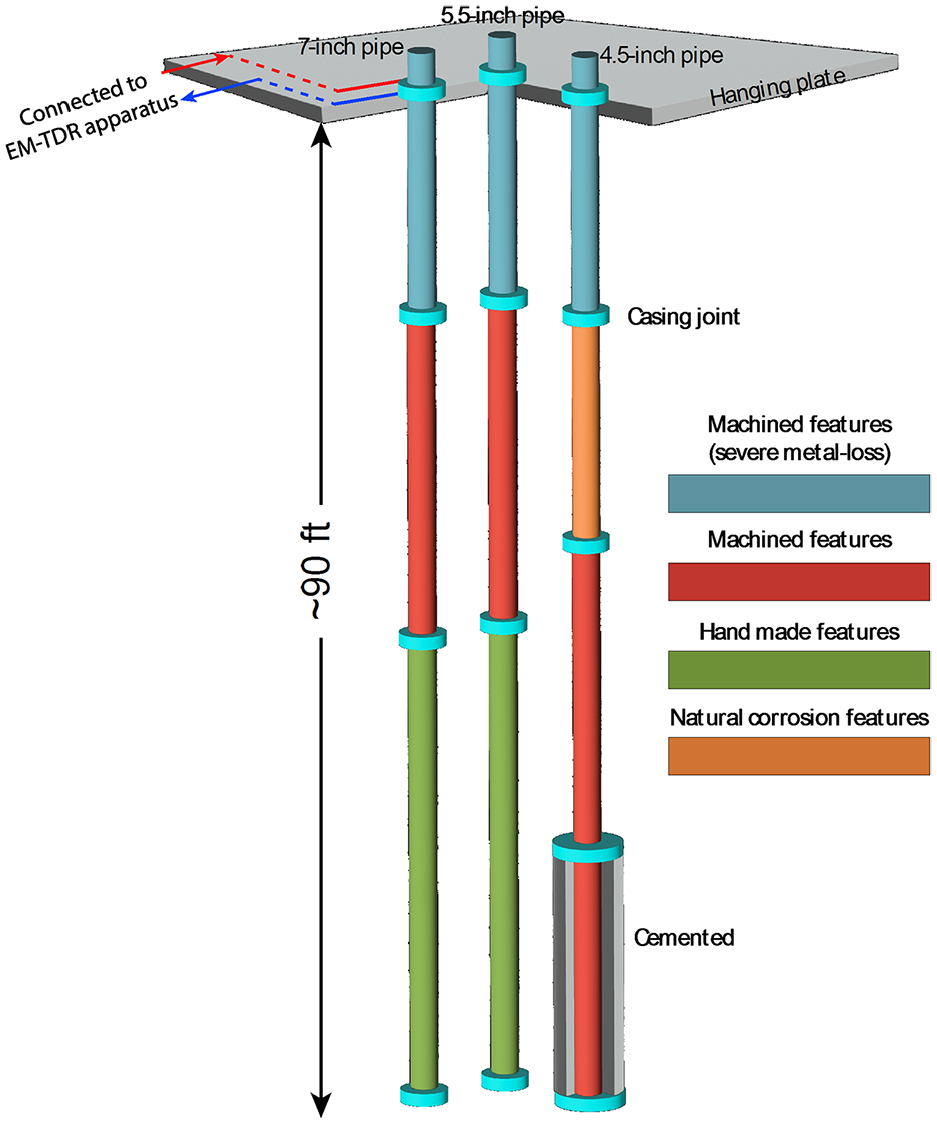
Schematic representation of the EM-TDR double-blind test conducted at the Deep-Well simulator, based on the ground truth revealed after completing measurements and interpretation. The Deep-Well simulator has a total depth of 150 feet. Pipes were suspended from the surface hanging plate, not reaching the bottom of the Deep-Well simulator. The pipe length ranges from 80 to 90 feet. Pipe section numbers, lengths, and feature configurations were undisclosed prior to measurements and interpretation. Casing joints are highlighted in cyan. The EM-TDR apparatus was connected at the top of the pipe under testing, positioned below the first casing joint. The sending and receiving of EM waves are denoted by red and blue arrows, respectively.

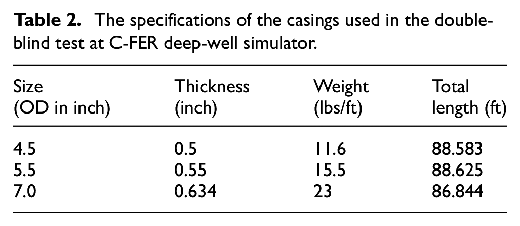
To ensure electrical separation between the casing strings, an insulation layer was placed between the casing strings and the hanging plate. The specifications of the casings are provided in Table 2. Note that this experiment was setup as a double-blind test, where the locations and nature of the degradation features were not known prior to the EM-TDR signal interpretation. Before the final interpretation delivery, the only available information about the casing strings pertained to their diameter, the number of sections, and the length of each casing string, which are typically known information for installed boreholes.

Table 2.

The specifications of the casings used in the double-blind test at C-FER deep-well simulator.

Size(OD in inch)	Thickness(inch)	Weight(lbs/ft)	Totallength (ft)
4.5	0.5	11.6	88.583
5.5	0.55	15.5	88.625
7.0	0.634	23	86.844

Disclosure after our interpretation submittal revealed a diverse range of complex metal loss features on the casings. These features included natural corrosion, machined pinholes, pitting, circumferential grooving, clusters of pitting, axial grooving, circumferential cutting, and handmade irregular-shaped features (Figure 10). According to the finite element simulation, all introduced features maintained a remaining burst strength of approximately 3000 psi, not compromised for the typical maximal operating pressure of underground natural gas storage wells.

During the tests, both the electromagnetic source and the oscilloscope were connected to the wellhead via coaxial cables. To capture potentially small-sized features and address attenuation challenges within each casing string, measurements were conducted across a frequency range of from 150 MHz to 2 GHz. Furthermore, to enhance the signal-to-noise ratio and suppress random electronic noise, the measurement was stacked 300 times during each data acquisition.

Ground truth

The laboratory test was designed to assess the effectiveness of the EM-TDR method in detecting various features, including both machined and natural corrosion features, with a complex distribution pattern on each casing. The machined features exhibit a wide range of sizes and shapes, including small pinholes, pitting, grooving, pitting clusters, irregular-shaped metal loss, circumferential metal loss, etc. Figure 11 presents photographs of some of these machined features, while Figure 12 shows the feature size distribution on the casings. Based on these data, the majority of the features have small surface sizes and shallow depths, with a few that are relatively long in the axial direction but narrow circumferentially, or wide in circumferential angle but short axially. In addition, there are deep and relatively large features, emulating severe integrity issues on all three sized casings.

Figure 11.

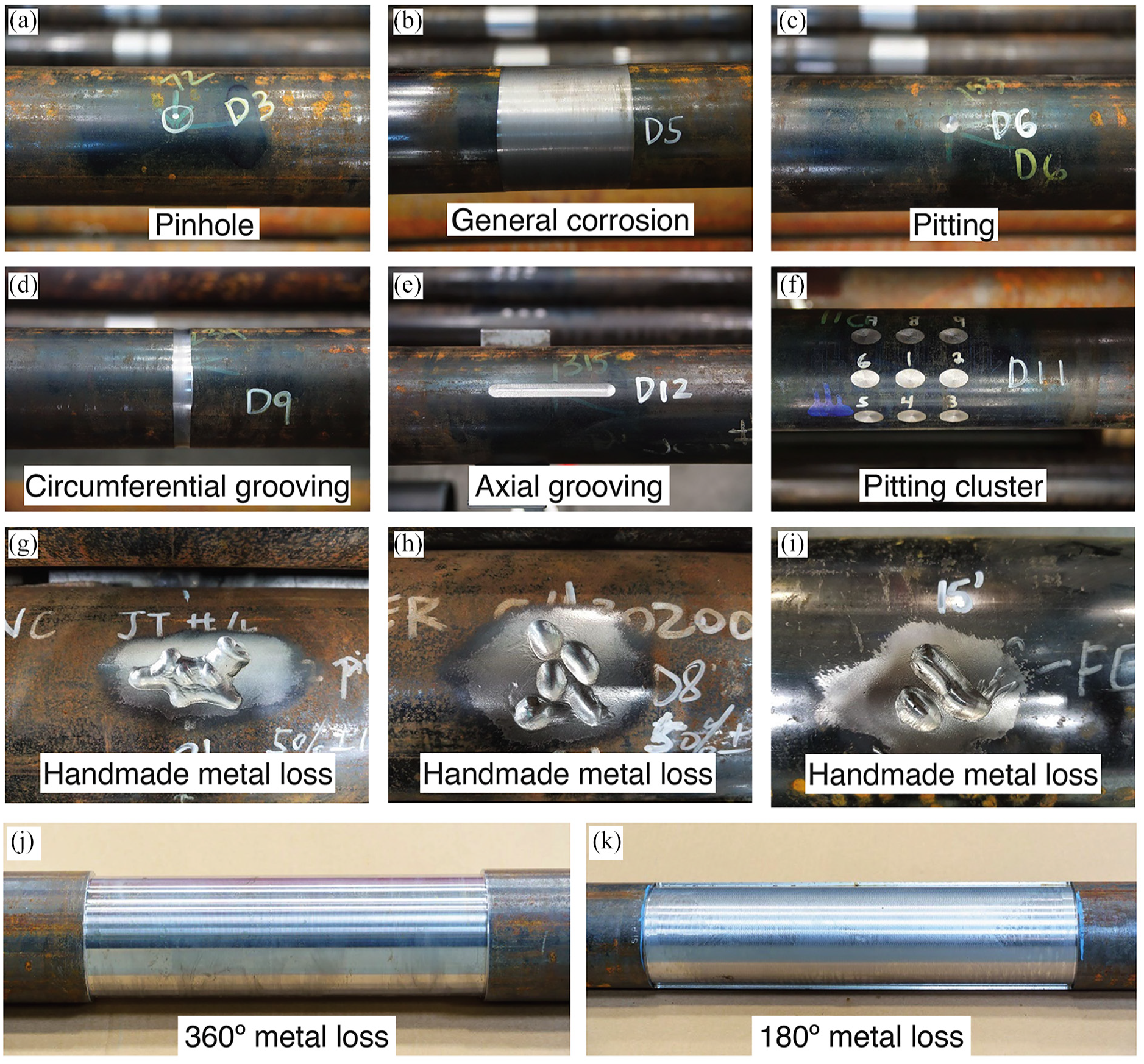
Photographs of the machined features used in the C-FER deep-well simulator double-blind tests: (a) machined pinhole, (b) machined emulated general corrosion, (c) machined pitting, (d) machined circumferential grooving, (e) machined axial grooving, (f) machined pitting cluster, (g) example of the handmade irregular-shaped metal loss, (h) example of the handmade irregular shaped metal loss, (i) Example of the handmade irregular shaped metal loss, (j) machined 360° metal loss, and (k) 180° metal loss.

Figure 12.

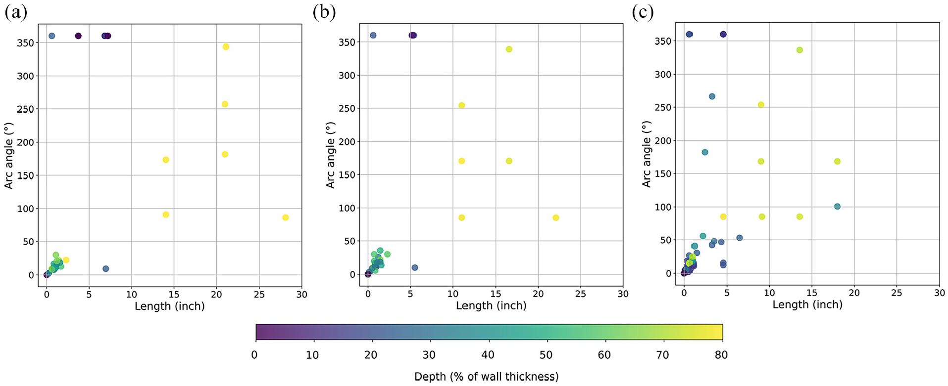
The size distribution of the features on the 7-inch (a), 5.5-inch (b), and 4.5-inch casing string (c). Vertical axis: width, in term of arc angle, of the features. Horizontal axis: axial length of the features. Color code: the deepest part of the features in term of percentage of the total casing thickness.

Figure 13 provides detailed statistical pie charts illustrating the distribution of features on 7-inch, 5.5-inch, and 4.5-inch casing strings, respectively. The inner pie charts in Figure 13 show the depth distribution of the features as a percentage of the casing thickness, while the outer pie charts illustrate the width of the features in terms of arc angle. The dimensions of the features cover the expected range of degradation in real-world scenarios. Over 60% of the features have a depth of less than 50% of the casing thickness, and more than 65% are narrower than a 45° arc angle. Given the dimensions of the casings (as shown in Table 2), most features are shallower than 0.3 inches and narrower than 2.7 inches. The shallowest feature is only 0.0315 inches on the 7-inch casing, 0.0194 inches on the 5.5-inch casing, and 0.0181 inches on the 4.4-inch casing. The smallest surface area is 0.0326 inch² on the 7-inch casing, 0.0294 inch² on the 5.5 inch casing, and 0.00617 inch² on the 4.5 inch-casing. These extremely small features are usually small pitting that belongs to pitting clusters (Figure 11(f)). However, as illustrated in Figure 11(a) and (c), there are singular pinholes and pittings in some other locations as well.

Figure 13.

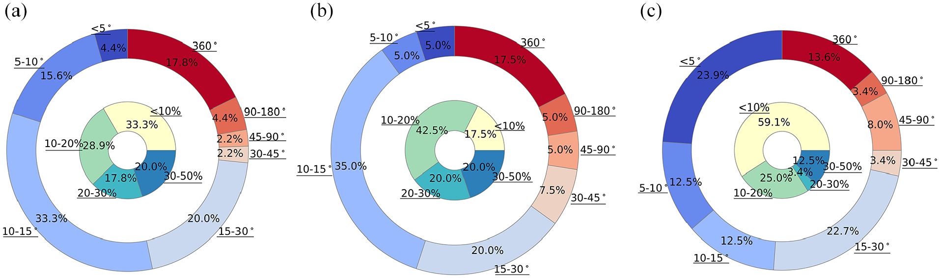
The feature statistical distribution on the 7-inch, 5.5-inch, and 4.5-inch casing strings presented as pie charts a, b, and c, respectively. The inner pie charts depict the feature depth statistical distribution, represented in terms of casing wall lost percentage (labeled by underlines). The outer pie charts illustrate the feature width statistical distribution, represented in terms of circumferential angle (labeled by underlines).

For the handmade irregular-shaped features (such as those in Figure 11(g)–(i)), only the deepest point and the length of the principal axis on the surface are known. The actual volumetric sizes of these handmade irregular-shaped features could be smaller than shown in the statistical charts. Additionally, one section of the 4.5-inch casing (orange section in Figure 10) consists solely of natural corrosion. Due to the irregular shape and size of the natural corrosion, quantitative statistics are not available for these features.

EM-TDR testing results

The resolution of reflected waves is primarily determined by the frequency of the source wavelet, and signal attenuation is governed by the number of cycles during propagation. While higher frequencies provide high resolution therefore essential for identifying smaller features, they suffer from higher attenuation. In contrast, lower frequencies can only distinguish larger features but have lower attenuation. Given that our EM-TDR acquisition covered various frequencies, we sought to identify reflections consistent across all frequencies or those merging into one large singular waveform at lower frequencies yet appearing as two separate smaller waveforms at higher frequencies. Reflections meeting these criteria are deemed likely to originate from actual features, including changes in casing material (both loss and increase, such as casing joints) and alterations in the surrounding dielectric media (e.g., water leakage in the surrounding formation or cement loss).

Figures 14 –16 illustrate the EM-TDR based feature identification results from the Deep-Well Simulator test conducted on 7-inch, 5.5-inch, and 4.5-inch casings, respectively. The data have been cross-correlated and reconstructed using the EMD method. As we know, from Rayleigh Criterion, that two events must be separated by at least half a cycle to be resolved. To solve for the feature width (Δd), it must satisfy Δd ≥ λ/4. For two closely spaced interfaces, the minimum resolvable distance is λ/4. Given that the velocity factor of steel is approximately 0.6, for the 1 GHz wave, the wavelength is around 19.7 inches (0.5 m), resulting in a minimum resolvable distance of 4.92 inches (0.125 m). For the 2 GHz wave, the wavelength is approximately 9.84 inches (0.25 m), resulting in a minimum resolvable distance of 2.46 inches (0.0625 m). Because most of the features for testing were relatively small in size, with dimensions less than 2.7 inches surface principle axial length, the 1 and 2 GHz source frequency were most suitable for identifying these features.

Figure 14.

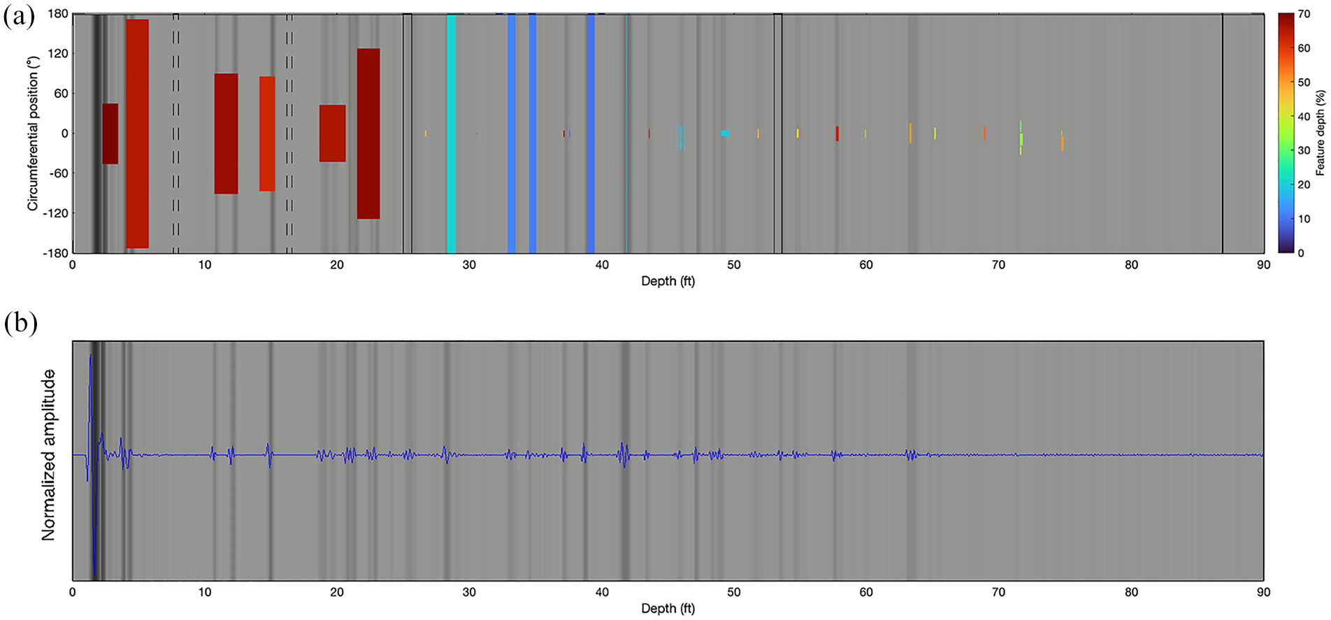
Comparison between the ground truth matrix and the reconstructed EM-TDR signal from the 1 GHz and 2 GHz signal on the 7-inch pipe: (a) the ground truth matrix overlays the reconstructed EM-TDR signal in the gray scale. The depth of the feature is represented via the percentage of the pipe thickness in color code. The background reconstructed EM-TDR signal is converted to the envelope form and plotted in the gray scale. The vertical dash lines represent the flush threads that connect pipe module sections. The double solid lines represent the casing joints. The single solid line at the end of the panel represents the end of the pipe. The vertical axis represents the circumferential width of the features (from −180° to 180°). (b) the reconstructed EM-TDR signal in analytical (blue) form overlays the reconstructed signal in envelope grey scale form (background).

Figure 15.

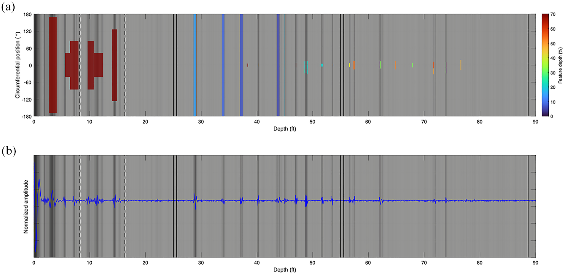
Comparison between the ground truth matrix and the reconstructed EM-TDR signal from the 1 GHz and 2 GHz signal on the 5.5-inch pipe: (a) the ground truth matrix overlays the reconstructed EM-TDR signal in the gray scale. The depth of the feature is represented via the percentage of the pipe thickness in color code. The background reconstructed EM-TDR signal is converted to the envelope form and plotted in the gray scale. The vertical dash lines represent the flush threads that connect pipe module sections. The double solid lines represent the casing joints. The single solid line at the end of the panel represents the end of the pipe. The vertical axis represents the circumferential width of the features (from −180° to 180°) and (b) the reconstructed EM-TDR signal in analytical (blue) form overlays the reconstructed signal in envelope gray scale form (background).

Figure 16.

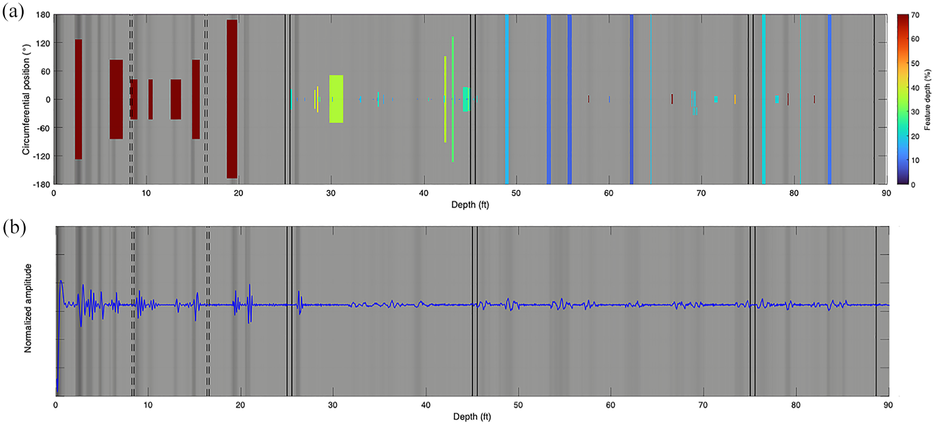
Comparison between the ground truth matrix and the reconstructed EM-TDR signal from the 1 GHz and 2 GHz signal on the 4.5-inch pipe: (a) the ground truth matrix overlays the reconstructed EM-TDR signal in the gray scale. The depth of the feature is represented via the percentage of the pipe thickness in color code. The background reconstructed EM-TDR signal is converted to the envelope form and plotted in the gray scale. The vertical dash lines represent the flush threads that connect pipe module sections. The double solid lines represent the casing joints. The single solid line at the end of the panel represents the end of the pipe. The vertical axis represents the circumferential width of the features (from −180° to 180°) and (b) the reconstructed EM-TDR signal in analytical (blue) form overlays the reconstructed signal in envelope gray scale form (background).

To evaluate the accuracy of the EM-TDR results, the ground truth was color-coded in terms of thickness loss and plotted in the top panels of Figures 14 –16. The double solid lines represent the casing joints, corresponding to the cyan cylinders in Figure 10.Warmer colors represent deeper metal loss. It is important to note that the ground truth plots in Figures 14(a)–16(a) are based on the major principal dimension of the features, that is, the longest axis on the surface and the deepest part of the features. The actual shapes of most features are more irregular, as seen in the pittings and irregularly shaped features shown in Figure 11. In the background, the reconstructed EM-TDR signal is depicted in amplitude envelope form in grayscale. The bottom panels (Figures 14(b)–16(b)) display blue traces representing the analytic form of the reconstructed EM-TDR signal overlaid on the amplitude envelope form of the reconstructed signal. Reflections from the casing joints (represented as cyan cylinders in Figure 10) and the bottom of the casing are predominantly characterized by large and wide waveforms. During the EMD process, these reflections are well separated in higher-order IMFs, which are dominated by slow oscillations. The locations of these casing joints were already known and are irrelevant in the context of integrity diagnosis. Furthermore, reflections from these casing joints tend to obscure smaller reflections from potential features close to the joints. To enhance the clarity of reflections from nonjoint features, during the signal reconstruction process, we excluded the slow oscillation IMFs containing reflections from the casing joints. Similarly, IMFs containing reflections from the bottom of the casings were also not used in the reconstruction process. Only IMF3 and IMF4 were used for the reconstructed data.

Upon initial examination of Figure 14 through Figure 16, it is evident that the reconstructed EM-TDR signal exhibits notable correlations with the ground truth across most locations. These correlations are particularly pronounced in reflections originating from the vicinity of the wellhead and areas with substantial metal loss. Given the wide variety of features in terms of size, depth, and shape across the three casings, the EM-TDR responses from these features will be examined in more detail.

Severe metallic loss

As shown in the schematic diagram in Figure 10 and the ground truth plots in Figure 14(a) through Figure 16(a), the features in the first segments of all casing strings are relatively deep and wide. The features are either wider than 180° angle or deeper than 30% of the casing thickness, or both. Photographic examples of these features are shown in Figure 11(i) and (j). The EM-TDR signals from these features not only have the largest amplitude but could also reveal the entry and exit anomalies from a particular feature, for example, the large feature at 10 ft deep in Figure 12(a), due to the high resolution of the signal.

Shallow and circumferential grooving

For the shallow features that are short in the axial direction, but wide in the circumferential direction, the EM-TDR also shows promising correlations with the ground truth. A photographic representation of this kind of feature is shown in Figure 11(d). In the second segment of the 7-inch casing, at the depth around 28 feet, 34 feet, 35 feet, and 39 feet (Figure 14), the reconstructed EM-TDR signal matches well with the ground truth. At the depth of 42 feet, the feature is a circumferential grooving, with an axial length of 0.62 inches and a depth of 0.0602 inches (9.5% of the wall thickness loss of the 7-inch casing). On the reconstructed EM-TDR profile, the reflection corresponds well with the location of the circumferential grooving. However, the amplitude and the width of the waveform from this particular reflection are relatively large (Figure 14(b)). This is likely due to the overlapping of the true reflection from the circumferential grooving and multiple reflections from earlier reflectors, most likely from the severe metallic loss at 21.8 feet, which has an axial length of 21 inches and a depth of 0.22 inches (35% of the wall thickness loss of the 7-inch casing). The arrival time and reflected waveform align with this hypothesis. Similarly, the reflection from the circumferential grooving at 45 feet deep of the second casing segment of the 5.5-inch casing also overlaps with the primary multiple (the reflections that bounce once) of the first casing joint, thus the large amplitude in the recorded signal (Figure 15).

Good matches between the EM-TDR results and the ground truth are also observed for shallow and circumferential cutting on both the 5.5-inch and 4.5-inch casings (illustrated in the second casing segment of Figure 15, and in the second and third casing segments of Figure 16). On the 4.5-inch casing, although we find good matches between the EM-TDR signal and the ground truth for shallow circumferential cuttings, we could not achieve a similar match for circumferential grooving at 65 feet and 81 feet, respectively. These may be because the grooving at these two locations are too narrow, with the axial length of 0.63 inches and 0.625 inches, respectively.

Interestingly, the last segment of the 4.5-inch casing is cemented, causing an alteration in the surrounding dielectric media. In the EM-TDR data, we can see the reflection from the interface between cement and the air at a depth of 75 feet (Figure 16). It is necessary to emphasize that, without prior knowledge, it is impossible to distinguish whether the reflections are due to the cement–air interface or features on the casing. Apart from the reflections from the cement–air interface, we do not observe any noticeable effect on the EM-TDR data from the cement as the cemented features are also identified in a similar fashion when compared with no-cement sections.

Pitting and handmade irregular-shaped cluster

In sections where features are closely clustered, the reflected EM-TDR signals may merge and interfere with each other. A photographic representation of this type of feature is shown in Figure 11(f). Thus, it is challenging to distinguish individual features within the clusters. For example, in the pitting cluster on the 7-inch casing (the cyan cluster at approximately 47 feet in Figure 14(a)), the reflected waveform appears as a wide and complex pattern. A similar reflection is observed at about 48 feet on the 5.5-inch casing (Figure 15), and at approximately 69 feet on the 4.5-inch casing (Figure 16), where a single waveform is observed instead of multiple distinct reflections. These instances demonstrate the difficulty in resolving closely spaced features.

Another type of clusters comprises of small, irregular-shaped, handmade features with varying principal lengths and orientations, depicted in Figure 11(g)–(i). The EM-TDR reflections from these handmade clusters correspond well with the ground truth, such as at the end of the 7-inch casing, depicted in light green at approximately 72 feet in Figure 14(a). Although these features share the same axial depth (the distance between the center point of the feature and the top of the casing) on the casing, their transverse locations differ. However, due to the one-dimensional nature of the EM-TDR measurement, distinguishing individual features with identical axial locations, but different transverse positions becomes impossible. Consequently, the reflected signal appears as a single reflection (Figure 14(b)). Similarly, comparable reflections are encountered from the handmade cluster on the 5.5-inch casing at approximately 72 feet and 75 feet (Figure 15).

Natural corrosion

The second section of the 4.5-inch casing contains features caused by natural corrosion, characterized by highly random, and often overlapping corrosion spots. Figure 17 provides a detailed corrosion map illustrating this complexity. It is challenging to pinpoint individual corrosion spots accurately. In our interpretation, we estimated the ranges of potential corrosion zones, depicted as dashed boxes in Figure 17. These estimations closely align with most of the actual locations of natural corrosion. The EM-TDR method successfully identifies three severely corroded areas, spanning from 29 feet to 30.5 feet, at 42 feet, and at 43 feet (Figure 17). However, EM-TDR failed to detect one severely corroded area, spanning from 44 feet to 45 feet. This discrepancy highlights the limitations of the EM-TDR method in detecting all instances of severe corrosion, particularly when the corrosion spots overlap with other strong reflectors, such severe corrosion areas or casing joints.

Figure 17.

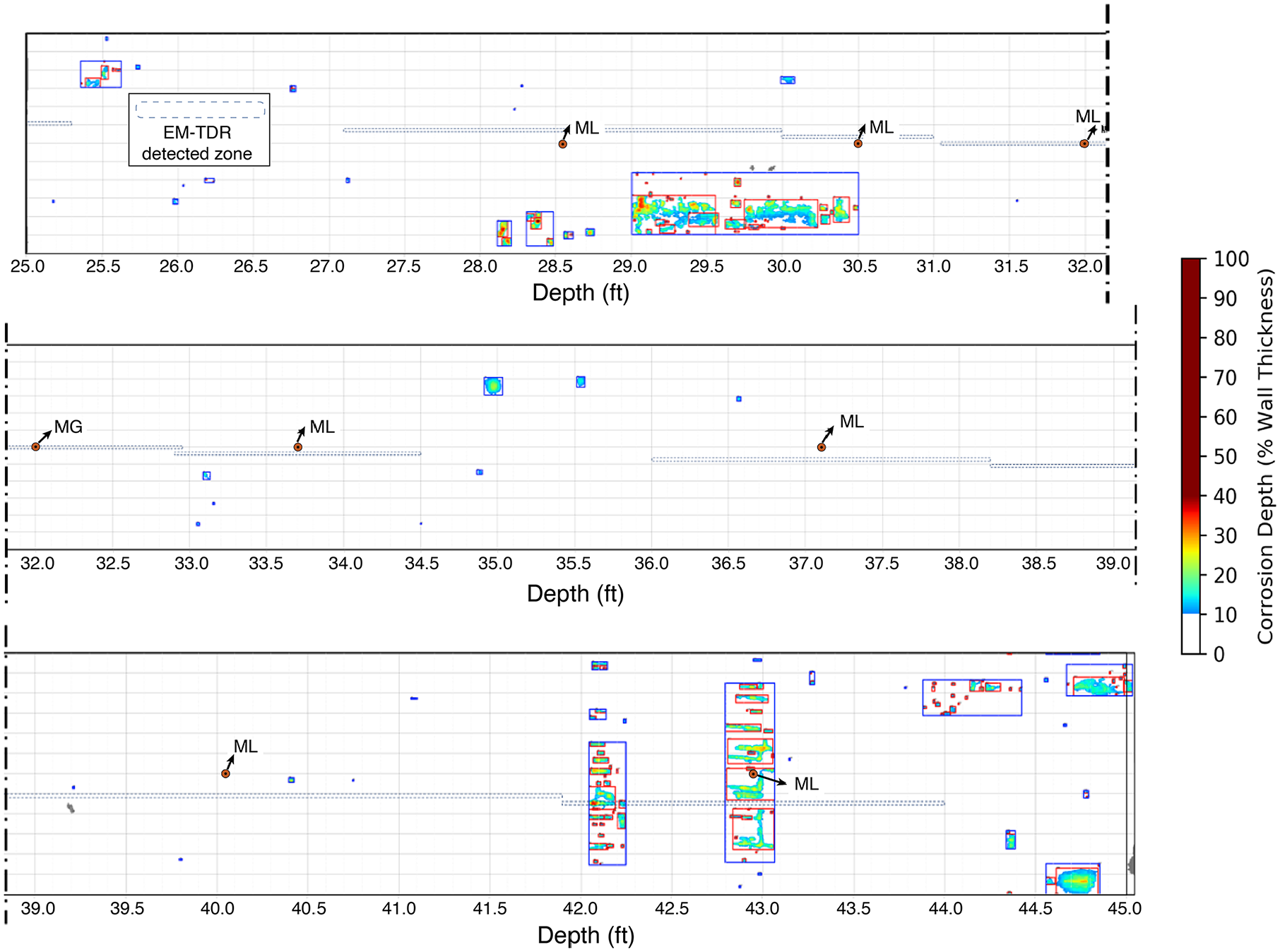
Alignment map between the EM-TDR interpreted features and the locations of natural corrosion.

Discussion

Results from the small-scale laboratory test demonstrate the feasibility of detecting small defects on metallic casings using the EM-TDR method, even when diameters of the features are as small as 0.5 inches. This test was used to validate the EMD method utilized for EM-TDR signal processing and noise isolation by demonstrating its capability to highlight the degradation feature while suppressing noise without generating artifacts.

In the double-blind test conducted at the Deep-Well Simulator of C-FER, the features were designed to emulate realistic scenarios of casing degradation, with a wide range of complex shapes, sizes, and distributions on the pipe. As demonstrated in previous sections, the EM-TDR measurements identified most of the feature locations. All features larger than 1 cubic inch were successfully detected using EM-TDR. For machined features smaller than 0.1 cubic inch, identification rates were 94%, 90%, and 93% for the 7-inch, 5.5-inch, and 4.5-inch casings, respectively. For features between 0.1 and 1 cubic inch, detection rates were 90%, 89%, and 83%, respectively. In the cemented segment of the 4.5-inch casing, 50% of features between 0.1 and 1 cubic inch were identified, and reflections from the cement–air interface were also observed. Among natural corrosion features, 63.5% were detected. Figure 18 illustrates the detected and missed features in terms of their volumetric metal loss and distance from the top of the casings, providing a summary of the performance of the EM-TDR method in identifying casing degradation features under realistic conditions.

Figure 18.

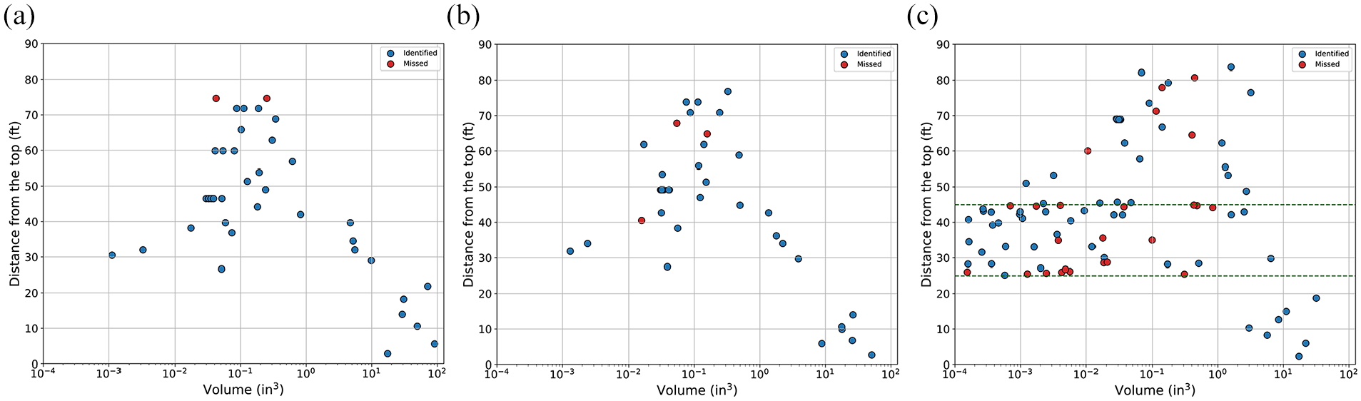
EM-TDR interpretation assessment in the perspective of feature location and the volumetric size: (a) interpretation assessment of the 7-inch casing, (b) Interpretation assessment of the 5.5-inch casing, (c) interpretation assessment of the 4.5-inch casing. The horizontal axis is in logarithm scale. The blue dots represent the features detected by the EM-TDR measurement. The red dots represent the features missed by the EM-TDR measurement. The green dashed lines indicate the top and bottom boundaries of the section with natural corrosion.

Figure 18(a) suggests that degradation feature identification accuracy for the 7-inch casing is the best, with only 2 out of 45 features missed by the EM-TDR measurements. These two missed features are small-volume pitting, less than 1 cubic inch, located at the end of the casing. However, other smaller features were successfully detected, likely because of their proximity to the source and receiver, and their grouping into larger clusters, making them easier for EM-TDR to identify. Similarly, as shown in Figure 18(b), the EM-TDR measurement on the 5.5-inch casing missed 3 out of 43 features. Two of these missed features are also located at the bottom of the casing, while the third is at a depth of 40 feet. Examining these EM-TDR results from a different perspective, we plotted the feature distribution in terms of surface size, depth, and distance from the top of the casing (Figure 19). Figure 19 indicates that the three missed features in the EM-TDR test on the 5.5-inch casing are among the shallowest. Similar to the missed features in the 7-inch casing, all three missed features in the 5.5-inch casing are singular pittings rather than being within a group (as indicated by their depth in both Figures 18(b) and 19(b)). The 4.5-inch casing contains a 20-foot-long segment with natural corrosion. As shown in Figure 18(c), most of the corrosion features are smaller than 0.1 inch³ in volume. In terms of surface size and thickness, as depicted in Figure 19(c), most of the corrosion spots are smaller than 1 inch² in surface size and shallower than 30% of the casing thickness. In segments other than the natural corrosion segment on the 4.5-inch casing, only four features were not detected by the EM-TDR measurements. Two of these missed features are circumferential grooves, and the other two are singular axial grooves. All of these grooves are shallower than 30% of the casing thickness (Figure 19(c)) and close to the end of the casing, consistent with the EM-TDR measurement accuracy from the other two casings.

Figure 19.

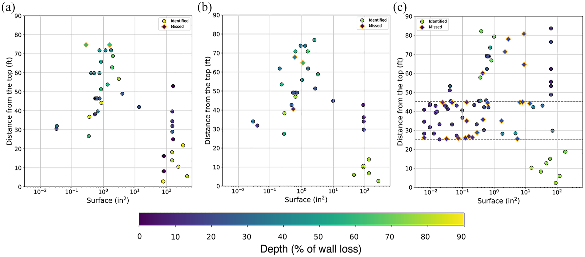
EM-TDR interpretation assessment in the perspective of feature location, surface area, and depth in terms of percentage of casing thickness: (a) interpretation assessment of the 7-inch casing, (b) interpretation assessment of the 5.5-inch casing, (c) interpretation assessment of the 4.5-inch casing. The horizontal axis is in logarithm scale. The circle-shape dots represent the features detected by the EM-TDR measurement. The diamond-shape dots represent the features missed by the EM-TDR measurement. The depth of the feature is color coded. The area between two green dashed lines represent the section with natural corrosion.

Similar to the small-scale laboratory test, while EM-TDR can identify the locations of most features on the casing strings, the exact axial lengths of these features are often indistinguishable due to limitations from signal attenuation and wavelength. Even though we utilized a 2 GHz signal, the main frequency component of most reflections is lower than 2 GHz due to attenuation. Consequently, while we can determine the depth of features causing the reflections, we are often unable to ascertain the size of the features. The two missed circumferential grooves, as discussed previously, are a result of resolution limitations. On the other hand, when features are close to the source, EM-TDR can potentially distinguish the axial lengths of the features. An example is the machined general corrosion at 11 feet on the 7-inch casing (Figure 14). The EM-TDR signal can clearly resolve the boundaries, for example, entry and exist, of this feature. However, in reality, it would be difficult to determine whether these corresponded to the two boundaries of single feature or reflections from two separate features unless clear signal polarity can be observed.

In the process of mapping the locations of the features, we assumed the travel time of the electromagnetic waves in the casing string to be constant. We first identify the reflections from the entry and end of the casing. Since we already knew the length of the casing, we calculated the velocity factor of the electromagnetic waves in the casings through the time–distance relationship. Then, using the derived velocity of the electromagnetic wave, we convert the two-way travel time to depth and located the interpreted features on the casings (Figure 14 through Figure 16). However, due to the subtle variation in both the casing string material property and the surrounding media, the speed of the electromagnetic waves may vary. As a result, the identified locations for some features are slightly off. For example, from the test result for the 7-inch casing (Figure 14), at around 25 feet from the wellhead, the reflected signal arrived earlier than the actual feature location (the yellow dot in Figure 14(a)).

These laboratory experiments also highlight some limitations in degradation feature detection using EM-TDR. First, the coupling-related impedance mis-match between the EM-TDR cables and the casing can generate secondary input wavelets. As shown in Figure 8, the reflections from double-bouncing are noticeable and may be misinterpreted as another reflector. Adding a resistor to the cable connected to the casing greatly attenuated the double-bouncing effect. However, the resistor also attenuated the high-frequency components, reducing resolution. In practical applications, reducing resolution may not always be desirable, indicating the need for careful interpretation or further engineering efforts to optimize signal entry coupling.

Furthermore, while we can clearly detect the location of defects on the casing, making a quantitative conclusion about the size of the defect based on EM-TDR reflections is challenging. This shortcoming is especially apparent for small defects, such as those in our laboratory tests. Despite electromagnetic waves being sensitive to metallic loss, the frequency used is not high enough to resolve the edges of defects. Consequently, we can observe reflections from the defects due to impedance changes but cannot distinguish the boundaries, thus the size, of those small features.

Another limitation of EM-TDR measurements is the potential for false-positive detections. Similar to the small-scale laboratory test, distinguishing between true primary reflections from casing degradations and multiple bouncing waves is challenging due to the one-dimensional nature of the measurement. For example, in the 7-inch casing measurement (Figure 14(a)), at around 48 feet, immediately after the cyan pitting cluster, a clear reflection is observed. Initially, we estimated it to be a reflection from a relatively large machined feature due to its comparatively higher amplitude. However, upon obtaining the ground truth, we realized it was only a harmonic reflection, that is, “echo,” from the first casing joint, leading to false-positive estimation. Similarly, at 40 feet on the 5.5-inch casing (Figure 15), a strong reflection is observed. Comparing this to the ground truth, there is indeed a shallow pitting at this location. However, it is unlikely that the pitting alone could generate such a strong reflection. More likely, the strong reflection observed at 40 feet is a combination of the reflection from the pitting and harmonic multiples from the severe metallic loss feature at around 15 feet (the last dark red feature in Figure 15(a)). At 5 feet on the 4.5-inch casing (Figure 16(b)), a cluster of reflections appears. These reflections result from multiple bounces between the waveform generator and the top of the casing due to poor coupling.

Conclusions

This study evaluated the precision of a novel application of EM-TDR technology and its data processing approach for identifying degradation features on metallic casings. To evaluate the performance of the EM-TDR method in realistic settings and quantitatively assess its accuracy with the support of ground truth data, we conducted both small-scale laboratory tests and double-blind laboratory tests using the Deep-Well Simulator facility at C-FER under well-controlled conditions. The results demonstrate the feasibility of using EM-TDR to diagnose casing integrity accurately and effectively. The key findings include

The small-scale laboratory tests with single defects indicated that small casing degradations as minimal as 0.5 inches in diameter and 25% of the casing thickness can be detected without severe attenuation effects.

The EMD method effectively separates useful reflections from noise without prior assumptions about the characteristics of the degradations, avoiding artificial anomalies.

The double-blind tests at the Deep-Well Simulator demonstrated high accuracy of the EM-TDR method in locating and evaluating casing damages, even in challenging scenarios with densely distributed features such as pitting clusters.

In segments with abundant natural corrosion, EM-TDR measurements correlated well with most main corrosion areas.

Reflections from the interface between air and cement in segments with cemented casing were observed, highlighting the potential of EM-TDR technology for wellbore integrity investigations and monitoring the surroundings of the casing.

While EM-TDR technology does not provide a comprehensive 3D depiction of wellbore conditions, its strength lies in its rapid and nonintrusive screening capabilities without the need to enter the well. Electromagnetic waves propagate close to the speed of light, allowing a single measurement, even with a 300-time stacking process, to be completed in seconds, ensuring a highly time-efficient process. Moreover, the EM-TDR method, based on the transmission of electromagnetic waves through metallic media, is readily applicable to the integrity monitoring of other metallic infrastructures, such as pipelines. As a complementary tool alongside existing high-resolution imaging/logging methods, EM-TDR is particularly suited for routine, expedited screening of energy infrastructures such as boreholes and pipelines. It can serve as an indicator technology that can trigger the need for more detailed and intrusive high-resolution logging/imaging inspections.

It is noteworthy that the EM-TDR method is still under development. Numerous challenges, both recognized and unforeseen, persist in real-world scenarios, including ambient noise interference and complex reflections from intricate pipeline or casing geometries (such as pipeline loops and borehole connections). Additionally, the physical properties of borehole construction methods and the surrounding geological formations can impact EM-TDR signals. Further laboratory and field tests are needed to further enhance this technology beyond the accuracy and feasibility study discussed here. Specifically, more field tests supported by ground truth data would significantly improve the EM-TDR technology toward a field deployable technology under complex conditions. In terms of signal optimization, utilizing time-multiplexed waveforms or broader-band frequency sweep waveforms could potentially enhance feature extraction in the future.

Footnotes

Acknowledgements

We thank the Pacific Gas & Electric Company (PG&E) for their support of the experimentation and the engineered tests conducted at C-FER Technologies in Edmonton, Canada. We also thank C-FER Technologies for conducting the simulated well tests.

Declaration of conflicting interests

The author(s) declared no potential conflicts of interest with respect to the research, authorship, and/or publication of this article.

Funding

The author(s) disclosed receipt of the following financial support for the research, authorship, and/or publication of this article: We are grateful for the funding support from the PIR program of California Energy Commission (CEC), and the Undocumented Orphaned Well project from Department of Energy’s Fossil Energy and Carbon Management Office.

ORCID iDs

Jiannan Wang

Yuxin Wu

Lingqing Luo

Government rights clause

This manuscript has been authored by employees of Lawrence Berkeley National Laboratory under Contract No. DE-AC02-05CH11231 with the U.S. Department of Energy. The U.S. government retains, and the publisher, by accepting the article for publication, acknowledges, that the U.S. government retains a nonexclusive, paid-up, irrevocable, world-wide license to publish or reproduce the published form of this manuscript, or allow others to do so, for U.S. government purposes.

References

Carey

JW.

Geochemistry of wellbore integrity in CO₂ sequestration: Portland cement-steel-brine-CO₂ interactions. Rev Miner Geochem 2013; 77: 505–539.

Wilt

Weiss

, et al. Wellbore integrity assessment with casing-based advanced sensing. Berkeley, CA (United States): Lawrence Berkeley National Lab (LBNL), 2021.

Johns

Blount

Dethlefs

, et al. Applied ultrasonic technology in wellbore leak detection and case histories in Alaska North Slope wells. In: SPE Annual Technical Conference and Exhibition, 2006, p.SPE-102815. SPE.

Johns

Aloisio

Mayfield

. Well integrity analysis in Gulf of Mexico wells using passive ultrasonic leak detection method. In: SPE/Iota Well Intervention Conference and Exhibition, 2011, p.SPE-142076. SPE.

Schultz

Robison

Bayh

III RI

, et al. Method and apparatus for placing and interrogating downhole sensors. U.S. Patent Application 10/178,188, 2002.

Cannon

Aminzadeh

. Distributed acoustic sensing: State of the art. In: SPE Digital Energy Conference and Exhibition. SPE, 2013, p.SPE-163688.

Boone

Ridge

Crickmore

, et al. Detecting leaks in abandoned gas wells with fibre-optic distributed acoustic sensing. In: IPTC 2014: International Petroleum Technology Conference, 2014, p.cp-395. European Association of Geoscientists & Engineers.

Hawkes

Gardner

Pressure transient testing for assessment of wellbore integrity in the IEAGHG Weyburn–Midale CO₂ Monitoring and Storage Project. Int J Greenh Gas Control 2013; 16: S50–S61.

Carey

Svec

Grigg

, et al. Experimental investigation of wellbore integrity and CO₂–brine flow along the casing–cement microannulus. Int J Greenh Gas Control 2010; 4: 272–282.

10.

Lowe

MJS

Alleyne

Cawley

. Defect detection in pipes using guided waves. Ultrasonics 1998; 36: 147–154.

11.

Alleyne

Pavlakovic

Lowe

, et al. Rapid, long-range inspection of chemical plant pipework using guided waves. Rev Prog Quant Nondestruct Eval Vol 20 2001; 20: 180–187.

12.

Wagner

Goncalves

Demma

, et al. Guided wave testing performance studies: Comparison with ultrasonic and magnetic flux leakage pigs. Insight-Non-Destr Test Cond Monit 2013; 55: 187–196.

13.

Zang

Z-D

, et al. Ultrasonic guided wave techniques and applications in pipeline defect detection: a review. Int J Press Vessels Pip 2023; 206: 105033.

14.

Wang

Wellhead based time domain reflectometry for casing integrity investigation. Int J Greenh Gas Control 2020; 96: 103002.

15.

Furse

Smith

Diamond

Feasibility of reflectometry for nondestructive evaluation of prestressed concrete anchors. IEEE Sens J 2009; 9: 1322–1329.

16.

Amir

Barzelay

Yefet

, et al. Condenser tube examination using acoustic pulse reflectometry. J Eng Gas Turbines Power 2010; 132: 014501.

17.

Topp

Davis

Time-domain reflectometry (TDR) and its application to irrigation scheduling. Adv Irrig 1985; 3: 107–127.

18.

Herkelrath

Hamburg

Murphy

Automatic, real-time monitoring of soil moisture in a remote field area with time domain reflectometry. Water Resour Res 1991; 27: 857–864.

19.

Heimovaara

Design of triple-wire time domain reflectometry probes in practice and theory. Soil Sci Soc Am J 1993; 57: 1410–1417.

20.

Wang

Stewart

Dyaur

, et al. Marine guided waves: subbottom property estimation and filtering using physical modeling data. Geophysics 2016; 81: V303–V315.

21.

Iskander

MF.

Electromagnetic fields and waves. Prentice Hall Upper Saddle River, 1992.

22.

Huang

Shen

Long

, et al. The empirical mode decomposition and the Hilbert spectrum for nonlinear and non-stationary time series analysis. Proc R Soc Lond Ser Math Phys Eng Sci 1998; 454: 903–995.

23.

Karan

Mahto

Sahu

. Intelligent speech processing in the time-frequency domain. In: Intelligent Speech Signal Processing, 2019, pp.153–173. Elsevier.

24.

Dragomiretskiy

Zosso

Variational mode decomposition. IEEE Trans Signal Process 2013; 62: 531–544.

Casing integrity diagnosis using wellhead-based electromagnetic time domain reflectometry: laboratory study