
Abstract
In vibration-based structural health monitoring (SHM), it is well known that environmental and operational variations (EOVs) affect the dynamic response of the structure of interest. This fact makes it difficult to distinguish between structural changes caused by damage and those caused by EOVs. In SHM, this issue is addressed by data normalisation, whereby machine learning techniques are commonly applied. However, ensuring their accuracy necessitates capturing a comprehensive range of EOVs within the training data. Collecting these is inherently challenging for real-world applications, especially with new EOV states emerging due to climate change. This study’s unique contribution is applying and comparing two grey-box models based on Gaussian process (GP) regression to remove EOVs with low data coverage and demonstrate their efficiency for damage detection with an open-access benchmark dataset. To this end, the first two bending mode natural frequencies – used as damage-sensitive features – of the Leibniz University Test Structure for Monitoring (LUMO), an outdoor lattice tower, are mapped. Two approaches to embedding physical knowledge in the GP are investigated. The first approach incorporates knowledge through the mean function, while the second involves the selection or design of a kernel. Subsequently, the two approaches are compared with a black-box and a white-box model. For long-term SHM, the repair of a damage mechanism is accounted for by the normal-condition alignment scheme, and damage detection is performed using the Mahalanobis distance. The study demonstrates that applying grey-box models contributes to a more reliable representation of the variations caused by unknown EOVs than pure black-box models, thereby improving damage detectability with sparse and incomplete training data due to climate change. However, as the dependencies modelled for LUMO are primarily linear, further research is required to assess the applicability of these findings to structures where dependencies are expected to be non-linear.
Keywords
Introduction
Structural health monitoring (SHM) employs various strategies to detect and identify structural damage. The damage identification process results in a hierarchical, five-level approach. 1 The lowest two levels are concerned with making reliable statements about whether damage has occurred and its location. The higher levels involve identifying the type of damage and prognosis for the remaining lifetime. A distinction is generally made between unsupervised SHM, which addresses the lower two levels, and supervised SHM for the higher levels. Following Farrar et al., 2 an SHM process generally involves the steps (a) operational assessment, (b) data collection, (c) feature extraction and (d) statistical model development for feature classification, whereby these steps are usually summarised by the statistical pattern recognition paradigm. During the feature extraction step, damage-sensitive features (DSFs), which are expected to correlate with damage-related changes in the structure, are extracted from the measurement data. The choice of DSFs is application specific. 3 Once appropriate DSFs have been selected, the subsequent feature classification step employs algorithms to determine the current state of the monitored structure. Unfortunately, for most civil engineering infrastructure, only data from the structure’s healthy state are available, resulting in an unsupervised learning SHM problem. Here, the DSFs are continuously extracted from the measurement data and compared with the healthy state of the structure. Any significant deviation can then be considered as indicating damage. However, environmental and operational variations (EOVs) can affect the structure’s behaviour and mask the DSFs. It can be stated that the more sensitive a DSF is to damage, the more sensitive it is to changing EOVs. 4 Handling these effects is commonly referred to as data normalisation and remains a challenge in the SHM research community. Considering the effect of climate change is crucial for a reliable data normalisation algorithm, as it will change the EOVs under which a structure operates over time. 5 Therefore, appropriate handling of the variations due to EOVs not included in the training data is essential to ensure the reliability of the SHM system. 6
In the case of global vibration-based SHM, it is assumed that the vibration characteristics under ambient, unknown excitation (output only, e.g., due to wind) of the considered structure change due to damage and can thus be utilised to obtain DSFs. A benefit of using a global method for damage detection is that the measurement locations do not have to be close to the damage. Here, natural frequencies are commonly employed as DSFs because they are physically tractable and can be extracted from dynamic measurements in near-real time due to the availability of established identification algorithms such as stochastic subspace identification (SSI) or Bayesian operational modal analysis (BAYOMA). Beyond this, spectral functions such as power spectra, 7 mode shapes, 8 transmissibilities, 9 autoregressive (AR) coefficients 10 and subspace-based indicators 11 can also serve as DSFs for vibration-based SHM methods. Although natural frequencies are not always sufficiently sensitive to damage, 4 they are selected as DSFs for this study as the focus is on data normalisation rather than on choosing the most sensitive DSFs.
Many authors have investigated the influence of EOVs on the natural frequencies of different structures. Farrar et al. 12 reported that the natural frequencies of the Alamosa Canyon Bridge vary by approximately 5% during 24 h. Peeters et al. 13 also indicated for the Z-24 bridge that for 1 year of monitoring, differences ranging from 14% to 18% in natural frequencies could be explained by EOVs. Ubertini et al. 14 reported variations in the natural frequencies of a bell tower due to temperature effects. Jonscher et al. 15 observed EOV-dependent variations in the natural frequencies for an operating onshore concrete-steel hybrid wind turbine tower of up to 7%. Similar variations due to EOVs were also identified for the natural frequencies of an offshore Vestas V90-3MW turbine on a monopile foundation, as reported in Weijtjens et al. 16 All these studies indicate that natural frequencies are susceptible to changing EOVs, which makes distinguishing between structural changes caused by damage and those due to changing EOVs challenging. Climate change will be another source of increasing variations in DSFs due to changing EOVs. Changing temperature and other dominant factors, such as flooding and high winds, significantly influence this variation. 17 However, the exact magnitude of the change is still unclear, whereby it is unquestionable that our climate is changing. 18 Therefore, numerous studies have investigated climate change’s potential impact on infrastructures.19–21 However, Figueiredo et al. 5 stated a research gap in the literature regarding the effect of unknown EOVs caused by climate change on long-term damage detection. Therefore, the authors of this study believe that vibration-based damage identification procedures will only become feasible in the face of climate change with adequate accounting for the new variations due to EOVs using robust data normalisation algorithms.
Several strategies have been proposed for developing a DSF insensitive to EOVs. 22 Currently, there are two well-known approaches for data normalisation. The first approach, and the one used in this study, is to measure the parameters related to EOVs and the structural response. The extracted DSFs of interest are then modelled as a function of the EOVs assumed to cause their variation. The second approach does not rely on measurements of the EOVs. Here, algorithms are applied directly to the DSFs to account for the influence of EOVs on them. Examples regarding the first approach are given by Dervilis et al., 23 who employed multivariate linear regression analysis to model the variation of natural frequencies with respect to EOVs for bridge monitoring. To compensate for EOVs using multivariate non-linear regression, Roberts et al. 24 modelled the natural frequencies of an operational Vestas V27 wind turbine blade based on temperature and wind speed. Other non-linear regression approaches use machine learning techniques such as artificial neural networks to normalise DSFs by modelling them as a function of EOVs. 25 Beyond this, Gaussian process (GP) regression has also been used in regression-based data normalisation. As a powerful Bayesian tool, GPs provide several desirable characteristics, including the ability to make predictions and probability distributions without specifying a particular parametric functional form, requiring only a few a priori inputs, and being capable of modelling signals with high levels of noise. 26 In this context, Worden and Cross 27 utilise an extended GP to map the variations in natural frequencies due to temperature for the SHM of the Z24 bridge. Jonscher et al. 8 used a heteroscedastic GP for data normalisation of the modal parameters of an onshore wind turbine tower to account for input-dependent noise.
As mentioned above, the second approach for data normalisation relies solely on the DSFs and does not require measurements of the EOVs. Here, Lucà et al. 28 apply the Mahalanobis squared distance to multiple modal parameters to filter out variations due to EOVs and enable damage detection as a multivariate outlier detection problem. Yan et al. 29 leveraged local principle component analysis as an extended version of principle component analysis (PCA) to cluster natural frequencies into linear regions based on their temperature conditions. Cointegration was also applied to spectral lines from the frequency spectrum to make these insensitive to temperature-induced variations. 30 In addition to this, Figueiredo et al. 31 compared an auto-associative neural network, factor analysis, Mahalanobis distance and singular value decomposition to distinguish between changes in the AR coefficients caused by EOVs and those caused by damage. Here, the Mahalanobis distance-based algorithm was identified as the most effective overall approach to data normalisation.
However, despite the availability of large amounts of structural and EOV data, it is often impossible to fully capture all possible states of a structure under the influence of those EOVs. Instead, the data provide information across a specific window of EOVs. This especially applies to the advanced machine learning approaches in regression-based data normalisation. Although these are powerful tools for extracting unknown correlations from data, predictions for unknown EOV states are challenging. As climate change progresses and the average temperature changes over time, 32 robust algorithms will become even more critical for dealing with those changes. 33 Here, Figueiredo et al. 5 analysed the effects of climate change on the SHM of the Z-24 bridge and stated that traditional machine learning algorithms may not be robust enough to deal with those effects. The second category of data normalisation approaches—data projection methods—is more robust against limited EOVs’ variability in the training data, as they model the relationships between the DSFs themselves rather than directly modelling the influence of the changing EOVs on the DSFs. Therefore, it seems reasonable to extend the purely data-based regression approaches for data normalisation with knowledge about the primary correlations between EOVs and DSFs to lessen the reliance on fully capturing the complete EOV data and to make the subsequent damage detection robust to climate change effects using regression-based data normalisation.
In this work, prior knowledge is incorporated into a GP to form a grey-box model. 34 There are a wide range of ways to incorporate prior knowledge. For example, a physics-informed kernel can be derived to introduce prior knowledge, 35 or constraints can be incorporated into the GP since boundary conditions are often known in advance in many engineering fields. 36 A detailed overview of the different approaches is given in Cross et al. 37 In the context of SHM, several authors have previously demonstrated that grey-box modelling can significantly improve predictive accuracy despite this research area’s relative novelty. Jones et al. 38 presented a constrained kernel regarding the geometry of the structure of interest for damage localisation. The study of Haywood-Alexander et al. 39 shows how physical knowledge can be utilised by constructing different kernels to model ultrasonic-guided waves. Pitchforth et al. 40 presented a grey-box model for wave loading prediction by combining Morison’s equation and a GP. Möller et al. 41 explicitly encoded known dependencies between inputs and outputs into the GP via a prior mean function. Zhang et al. 42 also incorporate a linear relationship between cable extension and temperature as prior knowledge to predict the deck displacement of a cable-stayed bridge for monitoring the structure’s performance. To create a physically meaningful probabilistic power curve model of an operating wind turbine, Mclean et al. 43 also employed bounded GPs to account for the normalised predicted power constrained to a maximum rated power.
In conclusion, with regard to the application of grey-box models in SHM, these models show promising results. However, their applicability for damage detection has yet to be thoroughly investigated. This study extends the investigations of the grey-box modelling approach proposed by Möller et al. 41 for the data normalisation of the DSFs in terms of the natural frequencies of a lattice tower exposed to changing EOVs. Here, the Leibniz University Test Structure for Monitoring (LUMO) serves as the case study on which the investigations of this work are carried out. 44 This work’s primary contribution is applying and comparing two different grey-box approaches to remove EOVs in case of low EOV coverage in the training data to enhance the resilience to new EOVs, for example, due to climate change, for damage detection. The classification performance of the models is demonstrated using an outdoor benchmark structure, and the grey-box models are compared against a black-box and a white-box model, whereby the rates of true positive and false negative indications of damage determine the classification performance.
The remainder of the study is organised as follows: section ‘GP regression’ briefly surveys GP regression as a solely data-driven method (or black-box model). After presenting GP regression, the introduction of GP-based grey-box modelling is initiated. Here, two approaches are discussed to embed physical knowledge as proposed solutions to model the effects of the EOVs on the natural frequencies selected as DSFs. The first approach is to incorporate prior knowledge into the GP by designing or selecting an appropriate kernel to embed a belief of which kind of functions the solution of the GP is drawn. The second approach is to include prior knowledge in the prior mean of the GP. Throughout the paper, LUMO is used to demonstrate the efficiency of the proposed models. In the section ‘Case study’, details of LUMO are offered, and its natural frequencies are presented as DSFs that show variability due to EOVs in terms of changing temperature and wind speed. In order to compensate for the influence of the EOVs on the DSFs, a comparative study of the black, white and grey-box models, using sparse and incomplete training data, is conducted. The section concludes with an investigation of the efficiency of the models for three different damage scenarios carried out on LUMO. Finally, the section ‘Conclusion and outlook’ presents a conclusion and discussion of the analysis carried out in this study.
GP regression
A GP model is designed for regression problems of the form

To make predictions, Bayesian inference is used. The prior, formed by
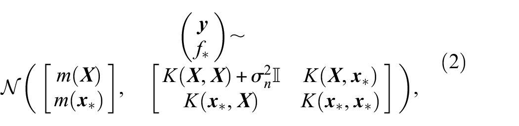
where
The kernel is always chosen as a function of the inputs
where

where the posterior predictive mean and variance are given by
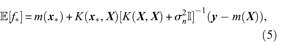
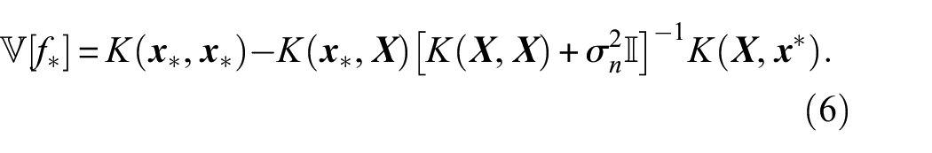
To predict the test targets
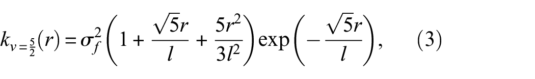
As shown in Equation (3), the Matérn 5/2 kernel has two hyperparameters:
where
When applying the exact inference for a GP on a data set of size
For this study, the variational approach to inducing variables of Titsias 49 is utilised. Following this, the posterior GP can be described by the predictive Gaussian distribution
where
Assuming that
where
According to,
49
it is useful for a good approximation to assume
All the models presented in this paper were written in Python and run using GPflow. 50
Incorporating prior knowledge
Following Cross et al.,
37
it is possible to incorporate prior knowledge into a GP in various forms. Here, it generally holds true that the more physical knowledge is incorporated, the less the predictions depend on the available data. Depending on how prior knowledge is integrated into the GP, the resulting grey-box model is more at the whiter end (much prior knowledge) of the spectrum of grey-box modelling possibilities or at the darker end (less prior knowledge, classical machine learning approaches).
37
For example, a GP with zero mean prior and a Matérn 5/2 kernel represents a black-box model and can be denoted as
As seen in Figure 1(a), this approach maps the trend within test data similar to the training data (it can be described as interpolation) well. However, as soon as the test data is beyond the observation range of the training data (described as extrapolation), the purely data-based GP can no longer predict the trend appropriately and falls back to its mean value of 0.
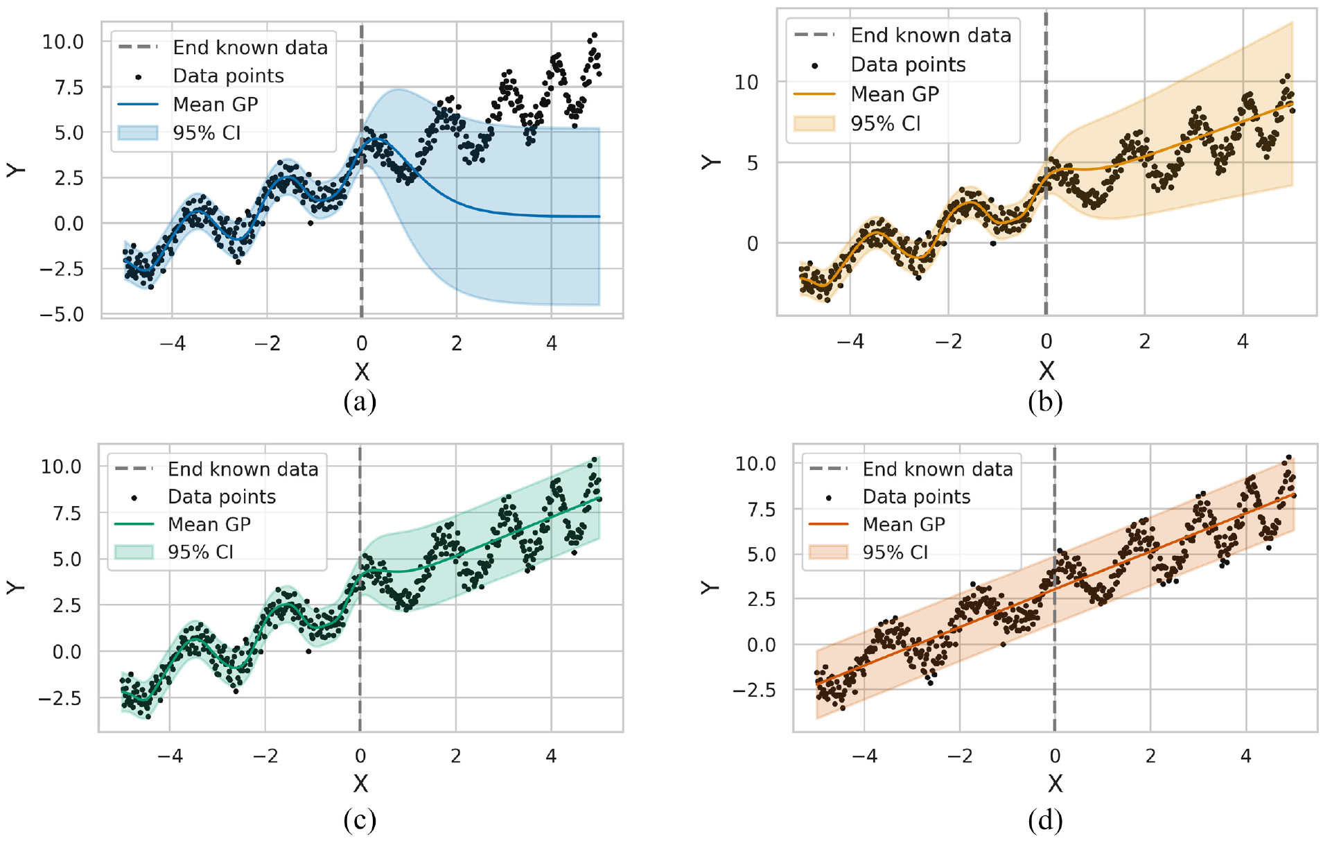
Interpolation and extrapolation of different grey-box approaches, including the 95% confidence interval (CI). (a) Shows the purely data-based GP:
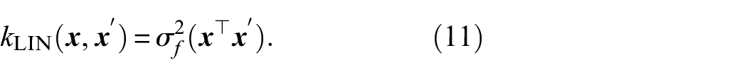
This study investigates two possibilities for incorporating prior knowledge into a GP. On the one hand, a GP with a kernel that combines knowledge-based and data-driven parts is used. This is particularly appealing if only little or partial knowledge of the process of interest is available. The resulting GP can be denoted as
On the other hand, a physics-based prior mean is utilised to account for prior knowledge. This approach becomes useful if parts of the mean behaviour can explicitly be expressed, and the GP is denoted by
Beyond the above-mentioned approaches, there is still a broad spectrum of methods for incorporating physical insights. For the example in Figure 1, it is conceivable to account for the periodic behaviour to obtain a better fit. Nevertheless, this can also lead to inaccurate predictions as the period and amplitude change. Thus, it seems reasonable to only map the underlying trend to minimise the risk of modelling errors. Therefore, the underlying trend is assumed to be linear. In the case of
By summing the kernels
As illustrated in Figure 1(c), the grey-box model
An essential idea behind machine learning is always to select the simplest model that best explains the underlying relation (Occam’s razor). Since a linear regression model is the simplest model that could be assumed for the example in Figure 1, this model can be used to evaluate the added value of the grey-box models under consideration. Figure 1(d) indicates that the linear model can capture the underlying linear trend, whereas non-linear effects cannot be captured by definition. In addition to the capacity to extrapolate the underlying linear trend, it is also vital to consider how well a model can cope with incomplete training data. For the evaluation, the
where
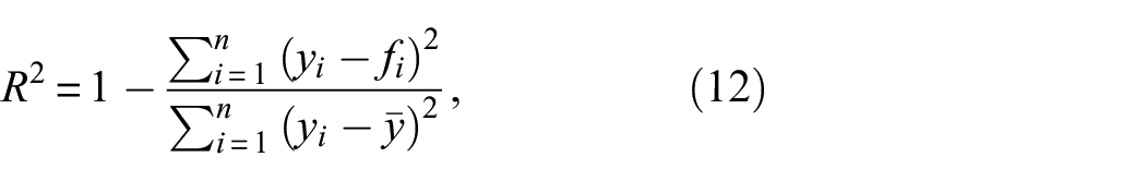
To this end, Figure 2 shows how a reduction of the training set affects the prediction accuracy of the models considered. For both Figure 2(a) and (b), the training set was reduced by removing equally distributed samples, so the proportion of the training set used is only up to 10% of the original training set.
Comparison of the
It can be seen in Figure 2(a), where the test data cover the same range of observations as the training data, that the size of the training set only has a minor effect on the accuracy, as the
However, as can be seen from Figure 2(b), such an approach cannot extrapolate, which resulted in negative
Case study
The Leibniz University Test Structure for Monitoring (LUMO) represents a benchmark structure for SHM methods. 52 The structure is a 9 m high steel lattice mast, shown in Figure 3(a). The mast consists of three identical sections with a length of 3 m each and weighs around 90 kg.
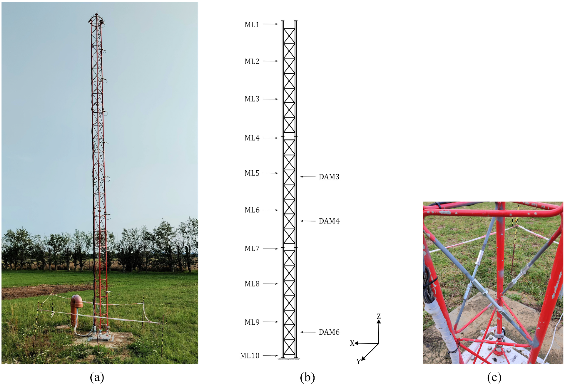
Photograph of the LUMO structure (a), a schematic of the structure highlighting the nine acceleration measurement levels (ML) and the investigated damage locations (DAM) with the reference axes (b), and the damage location 6 (DAM6) displaying the reversible damage mechanisms (c).
LUMO’s key advantage is the possibility of introducing a reversible local damage mechanism at six levels of the structure. Figure 3(b) depicts the locations relevant to this work. Removing up to three bracings (weighing 55 g each) at each damage level to introduce localised stiffness and mass changes is possible. The damage mechanisms include an M10 threaded rod with a coupling nut on each end. Damage is introduced by loosing the coupling nuts or removing the entire bracing. In this study, all considered damage cases involve the complete removal of one bracing at a certain damage level. Figure 3(c) shows the damage mechanism at level 6 (DAM6).
The structure is equipped with 18 uniaxial IEPE accelerometers mounted in pairs using 90° mounting brackets to measure orthogonal directions in the horizontal plane and capture spatial motion. The data is acquired at a sampling rate of 1651.61 Hz and stored in 10-min data blocks and can be accessed through a repository at Leibniz University Hannover. 44 Figure 3(b) shows the positions of the accelerometers that are positioned at ML1-9. The material temperature is measured at ML10 using a Pt100-type temperature sensor. It should be noted that this temperature is not expected to be spatially constant.
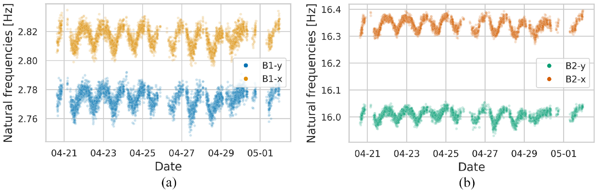
Beside the sensors on the structure, the Institute of Meteorology and Climatology (IMUK) of Leibniz University Hannover provides additional meteorological data from a meteorology mast close to the test structure. This data includes the air temperature, maximum wind speed, relative humidity, global radiation and wind direction. This study investigates the period from mid-April 2021 to July 2021. The corresponding natural frequencies of the first two bending mode pairs are pictured in Figure 4.
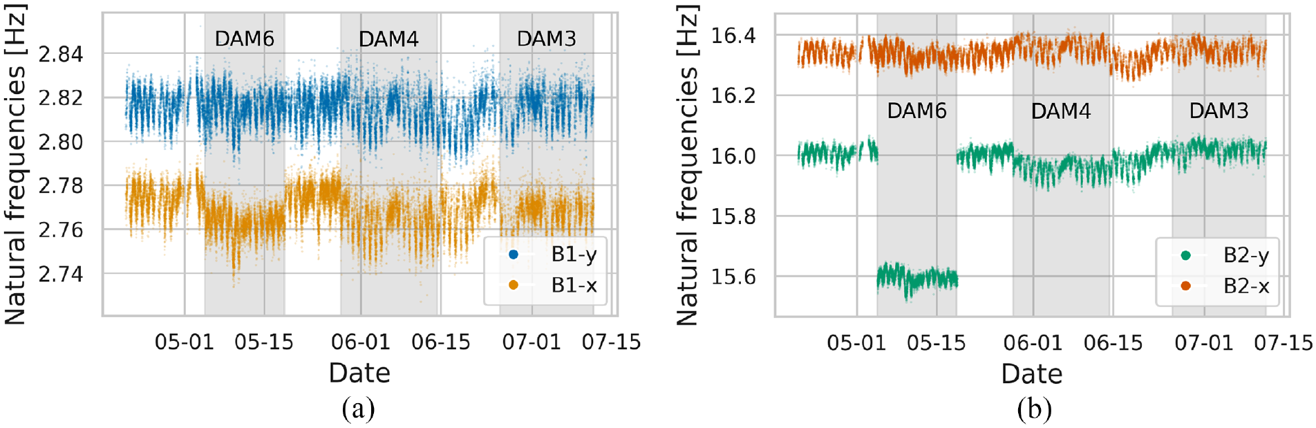
Evolution of natural frequencies for B1-x, B1-y (a) and B2-x, B2-y (b) for all states under study using 2-min intervals. The abbreviations B1 and B2 refer to the first and second bending modes, and x and y indicate the dominant orientation of the associated mode shape. Damage states are highlighted in grey.
This period covers a total of six different condition states of the LUMO. Descriptions of the condition state during this period are summarised in Table 1.
Health states of the structure and corresponding labels.
The states DAM6, DAM4 and DAM3 specified in Table 1 correspond to the damage locations pictured in Figure 3(b).
Increasing temperatures can be observed in the damage cases, representing variations in environmental conditions due to climate change in this study. To investigate the influence of increasing temperatures, which are not included in the training data, the regression approaches used in this study are only trained with data from state H. This represents the challenges of unknown environmental conditions due to climate change. This section first examines the damage-sensitive features—the natural frequencies of the first two bending modes—and their environmental variations. Afterwards, the data normalisation approaches are applied, and damage detection is performed.
DSFs and environmental variations
In order to assess the condition of a structure, DSF in terms of natural frequencies needs to be identified from the measurement data. This study uses the frequency domain method BAYOMA for this purpose. 53
As in previous studies regarding LUMO, torsional modes are excluded from the subsequent analysis. Despite their sensitivity in assessing damage states for LUMO, as evidenced by,54,55 torsional modes often do not present a high sensitivity to damage in operational civil structures, such as bridges and wind turbines. To develop an SHM system applicable to practical scenarios, it is reasonable to exclude them from this study. A similar finding regarding damage sensitivity also applies to higher natural frequencies, which tend to exhibit higher sensitivity to damage compared to lower frequencies. 4 However, due to a lack of excitation, higher modes can often not be reliably identified, and generally, more sensors are necessary to detect them with high fidelity. For larger structures such as bridges or wind turbines, the spatial resolution of sensors is often limited. Even for LUMO, it has been indicated that higher modes cannot be reliably identified using the current sensor setup. 44 Therefore, it is reasonable to utilise only the lower modes of LUMO in the subsequent analysis to obtain reliable identifications and to facilitate the transfer of findings to larger structures. Taking this into account, this study considers the first two bending mode pairs (B1-x, B1-y, B2-x and B2-y) to provide a realistic case study. These DSFs have also been studied by Jonscher et al. 54 concerning EOVs and damage detectability.
Besides the excitation, the time interval used for operational modal analysis is crucial for the accurate identification of the natural frequencies, as the identification uncertainty of these depends on the number of oscillation periods within the data set.
56
A comparison of the identification uncertainties
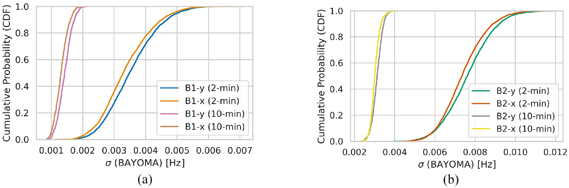
Cumulative distribution function (CDF) of the standard deviation
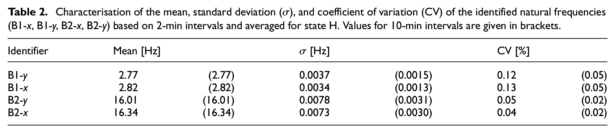
Hence, for the operational modal analysis of large structures such as wind turbines, 10-min intervals are commonly used.15,57,58 Regarding LUMO, Kahrger et al. 59 employed 2-min intervals to ensure better comparability of the findings obtained on LUMO with larger structures in terms of the number of oscillation periods within a dataset used for operational modal analysis. Therefore, this study is also based on the identification results of 2-min intervals. Table 2 characterises the natural frequencies obtained using BAYOMA during state H for 2-min and 10-min intervals.
Characterisation of the mean, standard deviation (
As LUMO is located outdoors, the structure is exposed to varying EOVs. In Figure 6, the variations of the considered natural frequencies can be observed for state H.
Evolution of natural frequencies for B1-x, B1-y (a) and B2-x, B2-y (b) during state H for a 2-min interval.
It can be assumed that material temperature and maximum wind speed significantly impact the structural behaviour of LUMO. 52 It should be noted that other EOVs can also be considered, as their selection is an application-specific modelling choice. Correlation analysis, in combination with a physical plausibility check, is often suitable for choosing EOVs that significantly influence structural behaviour. For instance, relative humidity was additionally considered for data normalisation of the natural frequencies of LUMO in Möller et al. 41 However, as it strongly correlates with temperature, it was not included in this study. Furthermore, in Kahrger et al., 59 global radiation was considered, which proved particularly useful for modelling predictive variance (cf. Equation (6)) as a function rather than a constant using heteroscedastic GP regression. Nevertheless, this study does not utilise global radiation since heteroscedastic GPs are not considered.
As noted above, variations in the natural frequencies of LUMO are primarily caused by temperature cycles that occur daily and seasonally.
52
Since Young’s modulus,
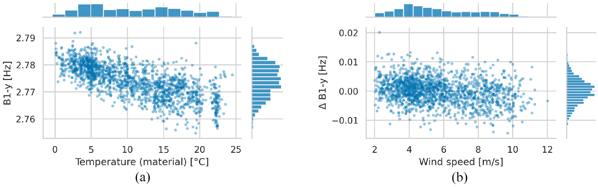
Correlation plots and histograms of the 2-min intervals for the natural frequencies B1-y versus material temperature(a) and wind speed (b) for state H.
Figure 7(a) clearly shows a linear relationship between the material temperature and natural frequency following the findings of Wernitz et al.
52
In this study, the Pearson correlation coefficient
As the wind speed measurements for the period under consideration were incomplete, the values were estimated using the methodology presented in Wernitz et al.
52
Since Wernitz et al.
52
noted that temperature variations mask the effects of wind speed, a linear regression was used to remove the fundamental linear trend of the temperature effects from the natural frequencies. Figure 7(b) depicts the influence of the maximum wind speed on the remaining residual
In conclusion, the influence of temperature on the considered natural frequencies is essentially linear and can be explicitly modelled for further investigations. However, a relationship with wind speed also exists, but to a significantly lower extent. Therefore, it seems reasonable not to explicitly specify this relationship as a linear function for the following investigations to avoid modelling errors.
Grey-box enhanced data normalisation
This study aims to make the first two bending mode pairs (B1-x, B1-y, B2-x, B2-y) as insensitive as possible to unknown EOVs using different grey-box-based data normalisation approaches. Furthermore, the study seeks to identify damage instances using the proposed data normalisation scheme. The grey-box models should enable meaningful predictions for EOV states not adequately represented in the training data, obtaining potentially robust algorithms to deal with EOV variability due to climate change. As stated in the section ‘DSFs and environmental variations’, the influences of material temperature and maximum wind speed cause the main variations of the natural frequencies. Hence, the grey-box models, introduced in the section ‘Incorporating prior knowledge’ should be investigated in terms of their applicability to mapping the EOVs to the natural frequencies as accurately as possible, especially with sparse and incomplete data.
Here, purely data-based model
Initially, an investigation is carried out to compare the accuracy of the grey-box models with each other, as well as with the purely data-based GP and the linear model for different-sized training sets for the state H. To this end, two cases are considered. Firstly, different subsets of the training data were created by removing uniformly distributed samples from the training data set (cf. Figure 8(a)). Secondly, the subsets were created by only considering samples up to a maximum temperature in the training set (cf. Figure 8(b)). For both, the accuracy of the models in fitting a test data set was compared in terms of their
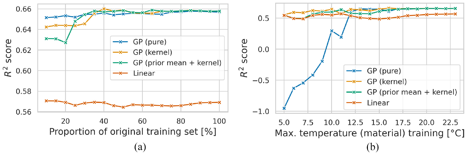
Evolution of the
Analysis of Figure 8(a) reveals that the
Nevertheless, a closer examination of Figure 8(a) indicates that the models demonstrate equivalent or superior accuracy to the purely data-based model when trained on larger data sets. This shows the effectiveness of employing grey-box models, as evidenced by the linear model showing the worst fit. Table 3 gives the accuracy of each considered model when the training data are complete (i.e., in the case of good EOV coverage).
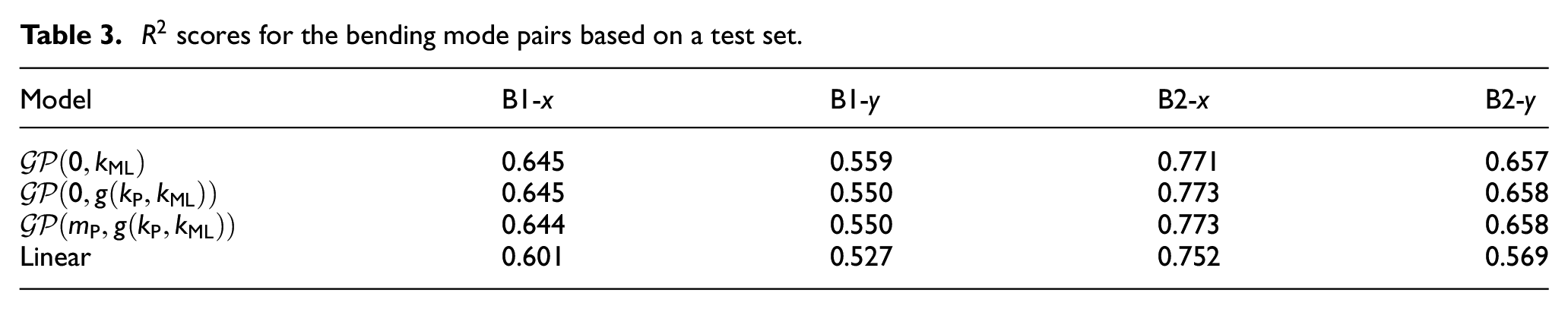
Table 3 reveals that the GP-based models perform almost equally for all natural frequencies and that the linear regression model always performs slightly worse than the others.
Figure 8(b) illustrates that the purely data-based GP can only map the trend above a certain limit with incomplete training data. The other models show a better extrapolation capability with incomplete training data regarding temperature coverage. When the EOV coverage is limited, it is noteworthy that the grey-box model
Furthermore, Figure 9 shows the predictions of the individual models for B2-y, whereby the training set only contains samples for which the material temperature is less than or equal to 11°C.
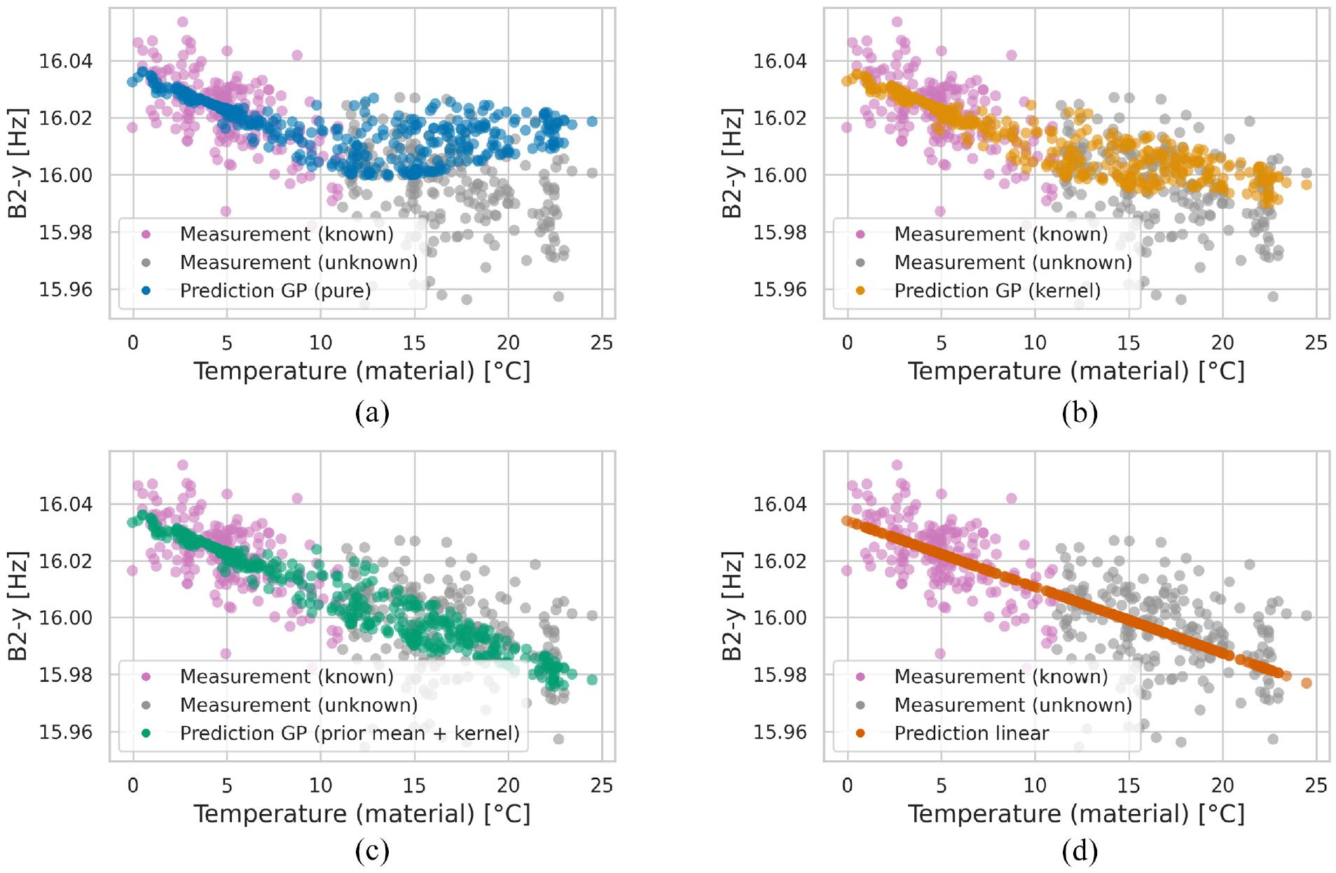
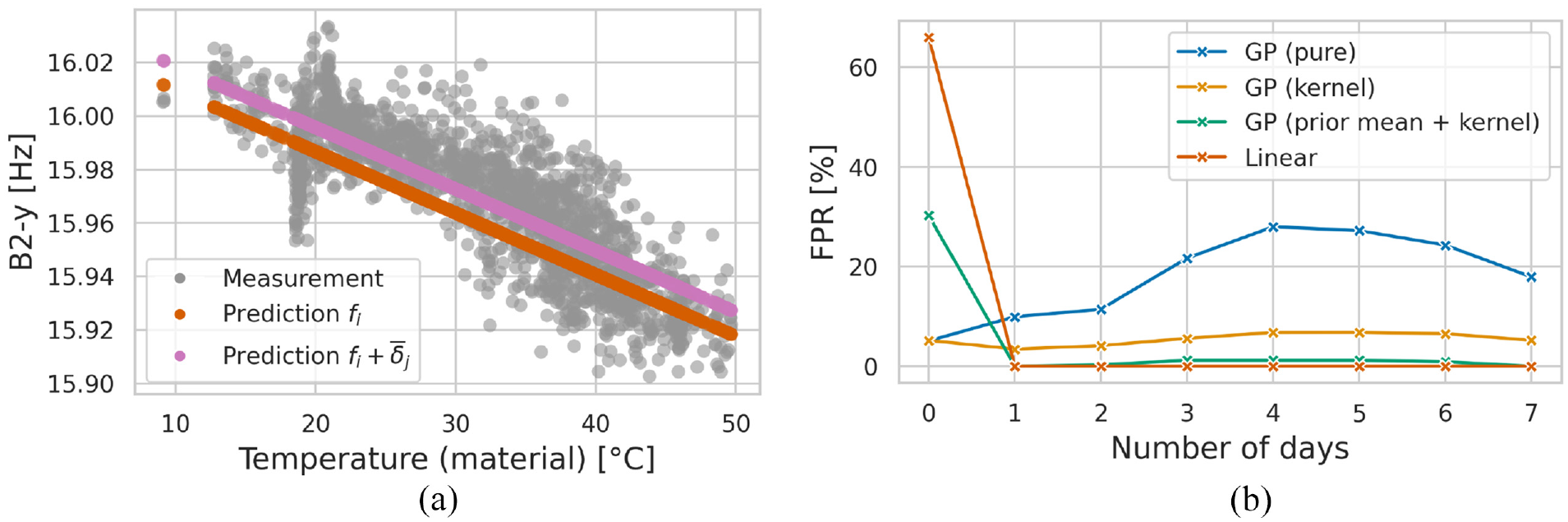
Predictions (interpolation and extrapolation) of the investigated models for B2-y on training data with a maximum material temperature of 11°C. (a) Shows the purely data-based GP as a black-box model:
In Figure 9(a), it can be seen that the purely data-based GP cannot extrapolate adequately. This model achieves an
In comparison with the purely data-based GP, the grey-box model
The grey-box model
Using a linear model (cf. Figure 9(d)), the overall
The findings presented above demonstrate that the grey-box model
Applicability in case of non-linear dependencies
As described in the previous section, the linear model performed well during the period considered in this study. This is mainly due to the linear relationships between the EOVs and DSFs. In general, however, non-linear correlations can also occur, as Peeters et al., 13 for example, found a bilinear behaviour between temperature and natural frequency for the Z-24 bridge, as the asphalt contributes significantly to the stiffness of the structure for negative temperatures. Wernitz et al. 52 found a similar behaviour for the natural frequencies of LUMO from December 2020 to March 2021 due to ice formation.
To demonstrate the proposed models’ applicability to model non-linear dependencies between EOVs and DSF, Figure 10 shows the prediction of the models considered in this study. The training data covers the period from 01 January to 23 February 2021. For the training, 80% of the available data was randomly selected, and only the temperature range from −10°C to 10°C was considered. The entire available temperature range was used for the test set (20% of the original data), for which the corresponding predictions (interpolation and extrapolation) can be seen in Figure 10. Furthermore, for
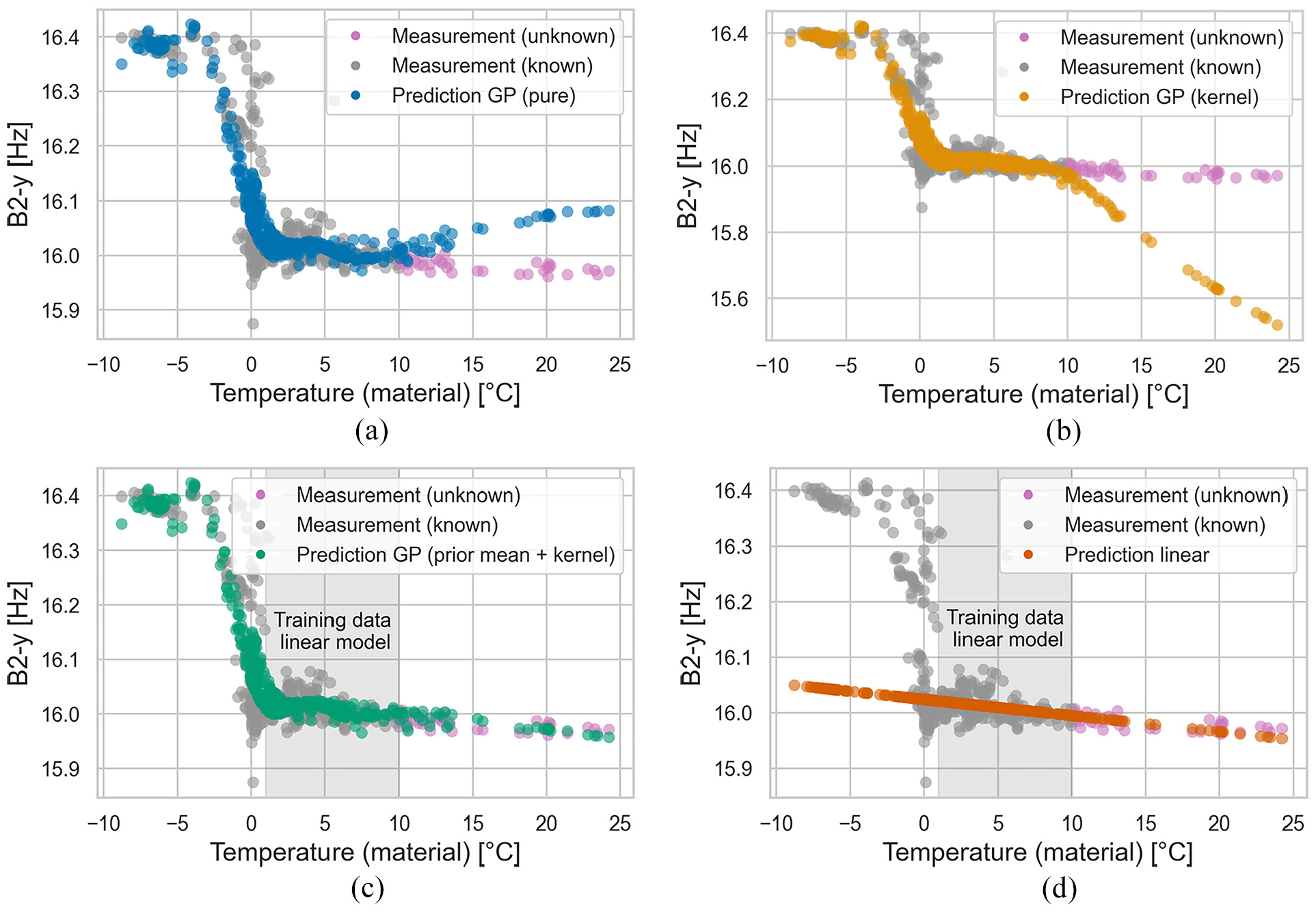
Predictions (interpolation and extrapolation) of the models under consideration for B2-y, including negative temperatures, demonstrate their applicability to model non-linear dependencies. (a) Shows the purely data-based GP as a black-box model:
Figure 10(a) shows that the purely data-based GP can map the non-linear dependency between temperature and natural frequency (
The same observation holds for the
Figure 10(c) demonstrates that the grey-box model
An interesting observation can also be seen in Figure 10. Here, the training data has two different trajectories around the freezing point, one steep and one less steep. The reason for this is the different behaviour of the structure for the thawing and freezing cases. All GPs used only map one of the cases. Strategies for mapping both cases can be the utilisation of a change-point kernel, 62 but this is not the aim of this study. It must also be mentioned that the non-linear relationship must be included in the training data; otherwise, the GP-based grey-box models cannot map this relationship correctly.
The linear model (cf. Figure 10(d)) is, by definition, not able to model the non-linear dependency. Therefore, the
The findings in this section demonstrate the ability of the proposed models to map non-linear relationships and how they can be adjusted for this purpose. However, since there are no suitable damaged states for LUMO from December 2020 to March 2021, it is not appropriate to use the corresponding data for the subsequent investigations.
Damage detection with incomplete data
Three damage cases (cf. Table 1) are investigated to demonstrate the effectiveness of the proposed grey-box data normalisation approach for damage detection for incomplete training data regarding missing temperature ranges, representing insufficient EOV coverage due to climate change. However, as stated in the section ‘Grey-box enhanced data normalisation’, the findings for incomplete training data can be transferred to the case of sparse training data. The data normalisation is combined with the Mahalanobis distance (MD) as a conventional multivariate outlier analysis method in SHM to perform damage detection. 63 It is well known that the accuracy of the MD is limited by the variability of the EOVs contained in the training data. Consequently, if the reference state of the MD differs in terms of the EOVs from the current, healthy state, this can result in a false-positive detection. However, precisely for this reason, the MD demonstrates the benefits of using powerful data normalisation methods. The MD is defined as:

Here,
For damage detection, the variations of the DSFs due to EOVs are removed by utilising the results of data normalisation via normal-condition alignment. Following Poole et al., 65 normal-condition alignment can be employed in the case of so-called domain shifts, for example, due to repair. 66 Here, a repair state’s first two statistical moments are aligned with the initial healthy state. As a result, an affine transformation and scaling are performed. The procedure to achieve this is as follows:
1. Standardise the data from the initial healthy state using,

where
2. Align the data from each repair state individually to the initial healthy state using,

where
Rather than estimating the statistical moments from the initially healthy state and repair state, the corresponding values
For damage detection, the MD is first calculated using the training set, and a threshold is set by determining the 99% CI based on the Monte Carlo method using 3000 samples. 63 During monitoring, the MD of each new data point is calculated. If the MD crosses the threshold, this point is presumed to be novel compared to the data used during training.
State H and DAM6 from Table 1 are used to investigate how the proposed data normalisation approach affects damage detection based on the above-mentioned procedure. The true positive rate (TPR) and false-positive rate (FPR) are used to judge the accuracy. The TPR is calculated as

where TP is the number of damaged data points classified as such, and FN is the number of incorrectly classified damaged state data points. The FPR is calculated as

where FP is the number of misclassified normal-condition data points, and TN is the number of correctly classified normal-condition data points.
As already depicted in Figure 4, this damage can be detected solely based on B2-y without further examination. Therefore, the TPR for all considered models is 100%. As stated in the section ‘Grey-box enhanced data normalisation’, grey-box models can be beneficial in the case of incomplete data. Therefore, this section builds upon the previous investigation by examining the impact of incomplete data on the FPR. The results are presented in Figure 11 for the states H and DAM6.
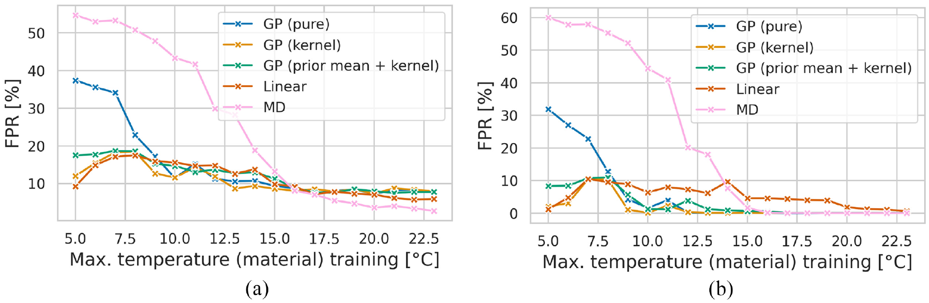
Evolution of the FPR for states H and DAM6 with incomplete data (a). (b) Shows the results when the moving average of the MD over the past 12 h is used. It should be noted that each data normalisation method is combined with the MD to perform multivariate outlier detection. The resulting FPRs are referred to as GP (pure), GP (kernel), GP (prior mean + kernel) and linear. The MD without data normalisation (referred to as MD) is also used here for comparison.
Figure 11(a) and (b) demonstrate that data normalisation with a purely data-based GP and MD exhibits an unacceptably high FPR when the degree of incompleteness within the training data is high, while the TPR remains at 100%. Therefore, the purely data-based model is not robust to unknown temperatures. Since a change in temperature due to climate change is to be assumed, a traditional machine learning method seems unsuitable for dealing with the effects of climate change. This finding aligns with the results of Figueiredo et al. 5
Figure 11(a) demonstrates that the MD can achieve a better FPR with sufficiently good EOV coverage compared to other methods. This is because the regression models involve modelling errors when removing the EOVs from the DSF according to Equations (14) and (15), whereas the pure MD does not include additional modelling errors. Conversely, the FPR of the linear model is equivalent to that of the grey-box models. This suggests that the primary influence of the EOVs on LUMO stems from the linear correlation between temperature and natural frequency. However, in the case of good EOV coverage, this model also shows a slightly lower FPR than the two grey-box approaches (cf. Figure 11(a)).
Figure 11(b) shows the result of applying a moving average of the MD over the past 12 h for robustness against identification errors and avoidance of false-positive detections. Therefore, a decision on whether damage has occurred is not made based on a single data point. As shown in Figure 11(b), it becomes evident that applying a moving average to the normalised MD positively affects the results compared to Figure 11(a). This observation suggests that they are more resilient to the effects of climate change. However, with improved data coverage, the purely data-based GP and the MD can match the FPRs of the grey-box approaches. However, without relevant experience, it is challenging to determine when this sufficiently large amount of data is available for a particular use case. In the context of SHM, encountering situations where only limited data on the normal state of the system are available is expected.
Table 4 demonstrates the impact of incomplete training data on the accuracy of damage detection using the proposed models for data normalisation, achieved by restricting the maximum material temperature occurring in the training data to 11°C. Notably, this temperature limit closely corresponds to the mean material temperature of 11.63°C for state H. Moreover, the mean material temperature for state DAM6 is 13.65°C, indicating a significant overlap between the training and test data.
Evaluation of classification performance in the case of using training data with a maximum material temperature of 11°C.
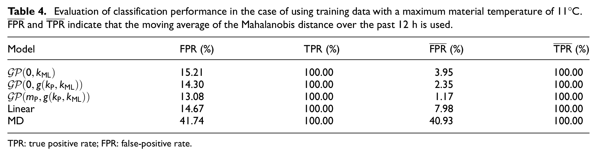
TPR: true positive rate; FPR: false-positive rate.
From Table 4, it is evident that both grey-box models demonstrate a significant improvement in the FPR when considering the moving average of the MD. The utilisation of grey-box models, combining their white-box and black-box parts, outperforms the models where only a black-box or white-box part is employed. Grey-box models prove particularly valuable when the limited training data still encompass a significant portion of the subsequent test data. In scenarios with unknown EOV regimes, these models predominantly fall back on their white-box part. Therefore, grey-box models generally enhance the performance of the white-box parts using additional data information while maintaining the white-box parts’ accuracy as a lower limit. This observation supports the adoption of grey-box models for data normalisation to better address climate change’s impact.
Damage detection and the repair problem under incomplete training data
Following the results presented in section ‘Damage detection with incomplete data’, where the effectiveness of the grey-box enhanced data normalisation approach in reducing the FPR when utilising the MD in the case of incomplete training data was demonstrated, the applicability of this approach as a long-term SHM method will now be investigated. For this purpose, the period from mid-April to July 2021, including the states listed in Table 1, will be studied, whereby all models are exclusively trained on data from state H. As shown in Table 5, the test data go beyond the observations included in the training data. The incompleteness within the training data thus provides a practical application case for grey-box models. Moreover, the test data’s temperatures are higher, representing climate change’s influence on SHM in this study.
EOVs for state H and without state H.
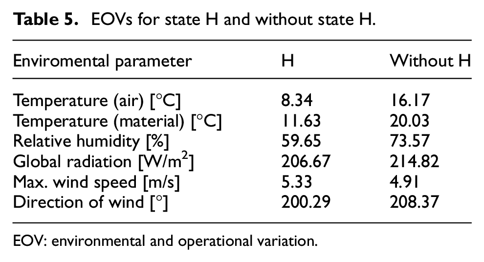
EOV: environmental and operational variation.
Before employing these, however, the importance of data normalisation methods is demonstrated by using MD without prior data normalisation for damage detection in Figure 12(a).
Application of the moving average of the pure MD for long-term SHM (a). The FPR and TPR for healthy and damaged states were found to be 12.33% and 66.29%, respectively. Utilisation of a linear model for data normalisation without addressing the repair problem in combination with the moving average of the MD (b). For all healthy and damaged states, the overall FPR is 35.06%, and the TPR is 97.67%.
When damage detection is solely based on the MD, Figure 12(a) shows that damage DAM3 is completely masked and cannot be detected. Furthermore, Figure 12(b) depicts the challenges that arise when repairs are conducted after each instance of damage, as the healthy data after the repair of DAM4 are misclassified as a novelty. While the damage mechanisms of LUMO were designed to be completely reversible, slight variations may occur during repair, leading to changes in the structural dynamics. This study assumes that repairs primarily impact the stiffness properties of LUMO, resulting in shifts in the natural frequencies as a constant offset. As shown in Equation (15), the normal-condition alignment utilises
The following procedure is implemented to tackle the repair problem while also minimising the training effort required for data acquisition and computational resources for data normalisation: As explained in Wickramarachchi et al.,
67
it is presumed that LUMO returns to normal conditions immediately after each repair and for the subsequent 7 days. The daily average offset

To account for the offset resulting from the repair, a prediction from a regression-based data normalisation method is aligned to the post-repair state by

Figure 13(a) illustrates the impact of correction via the offset
(a) Depicts the alignment of the predictions of the linear regression model for state R2 using the optimal offset
To obtain the optimal offset, the FPR for the first 7 days after the repair is calculated using each offset
As depicted in Figure 13(b), the optimal offset for obtaining the minimal FPR for state R2 is achieved using 1 day for the data normalisation models except for the purely data-based GP. In the case of the purely data-based GP, using an offset always leads to an increase in the FPR compared to when no offset is applied. This is due to the model’s inability to extrapolate well, as illustrated in Figure 9(a). This makes the correction with an offset ineffective. However, as illustrated in Figure 13(b), a slight increase in the FPR after 1 day becomes apparent for the other models under consideration. This phenomenon may be attributed to unusual EOV states affecting LUMO during this extended period, leading to either an overestimation or underestimation of the offset. The procedure for addressing the repair problem appears to be applicable. However, adapting the regression-based data normalisation models to the post-repair state leaves room for improvement for future research, although it is not the focus of this study.
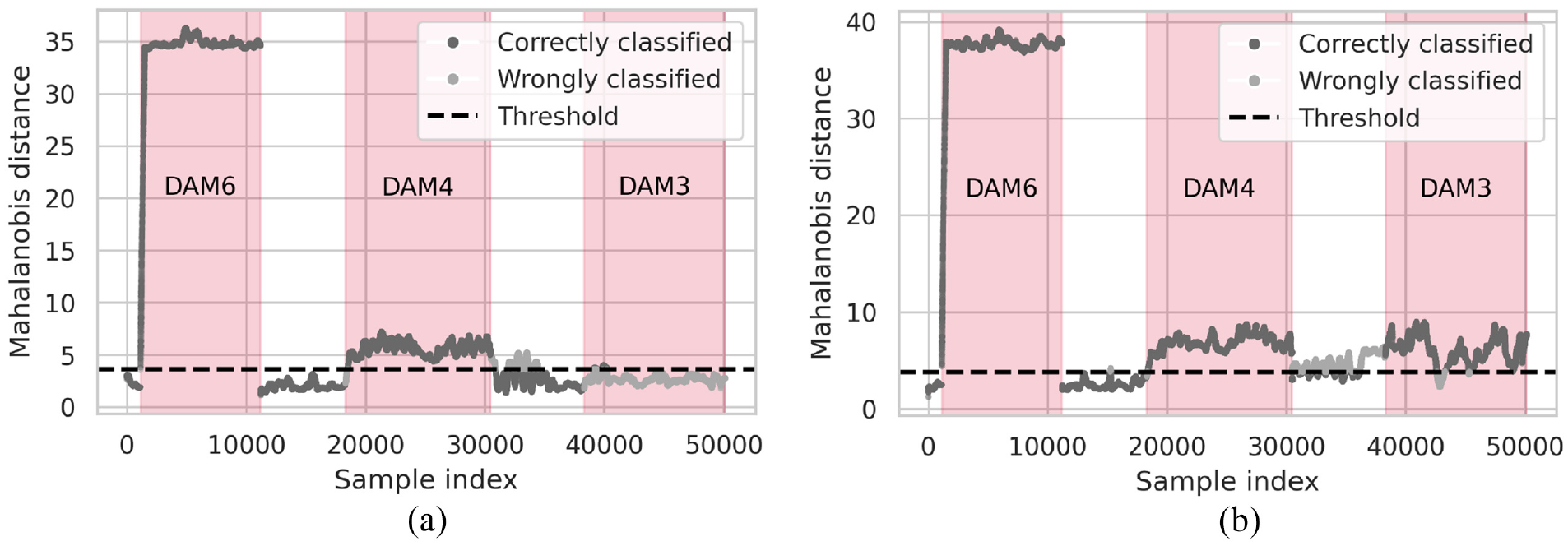
Using the methodology mentioned above to tackle the repair problem, the results of the subsequent damage detection are presented in Figure 14.
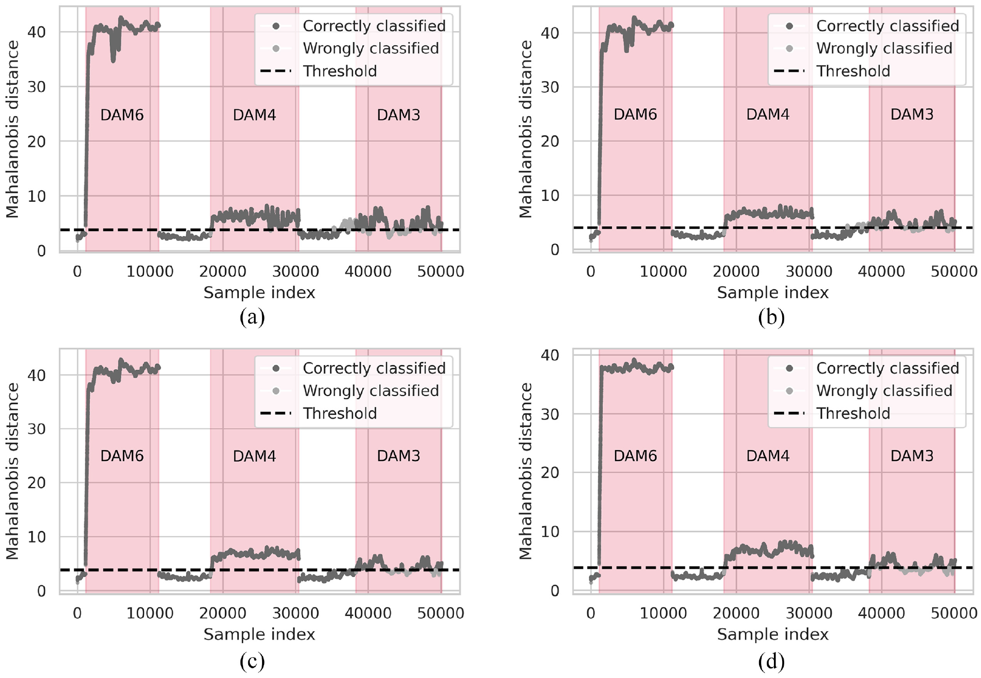
Results of the damage detection using different regression models for the data normalisation and the MD after applying a moving average of the past 12 h. (a) Shows the results for the purely data-based GP:
Figure 14 illustrates that DAM6 and DAM4 can be reliably detected with all proposed models, and the repair state R1 can be appropriately considered. However, in terms of damage detection, it can be observed that the influence of the damage on the MD decreases with increasing height of the damage position (see Figure 3(b)). This is because the first two bending mode pairs of the lattice tower structure are employed as DSFs. It should be noted that only one mode of each bending mode pair reacts significantly to damage, as the damage is asymmetric due to the activation of one damage mechanism. Regarding the relationship between damage location and its impact on DSFs, the first mode shape (see Ref. 52) indicates that the natural frequencies of the first bending mode pair are less affected by damage as height above the tower base increases. Furthermore, the damage mechanisms are located on the diagonal struts of the structure. With regard to DAM3, these struts are barely stressed for both bending mode pairs, which reduces their influence on the structure’s natural frequencies.
Concerning the data normalisation approaches employed for subsequent damage detection, it can be seen that when utilising the purely data-based GP in Figure 14(a), the threshold is exceeded before DAM3 is activated. This observation appears to be caused by the model’s poor ability to extrapolate to unknown EOV states. Therefore, whether the DAM3 damage was genuinely detected or was coincidentally identified due to insufficient data normalisation using this approach is questionable. This illustrates that rising temperatures, for example, due to climate change, can lead to false positives when using a black-box approach. In contrast, both grey-box models appear to be more capable of capturing the influences of these EOVs. Nevertheless, Figure 14(b) indicates that the grey-box model
When looking at the results presented in Figure 14, it is noticeable that the TPRs of
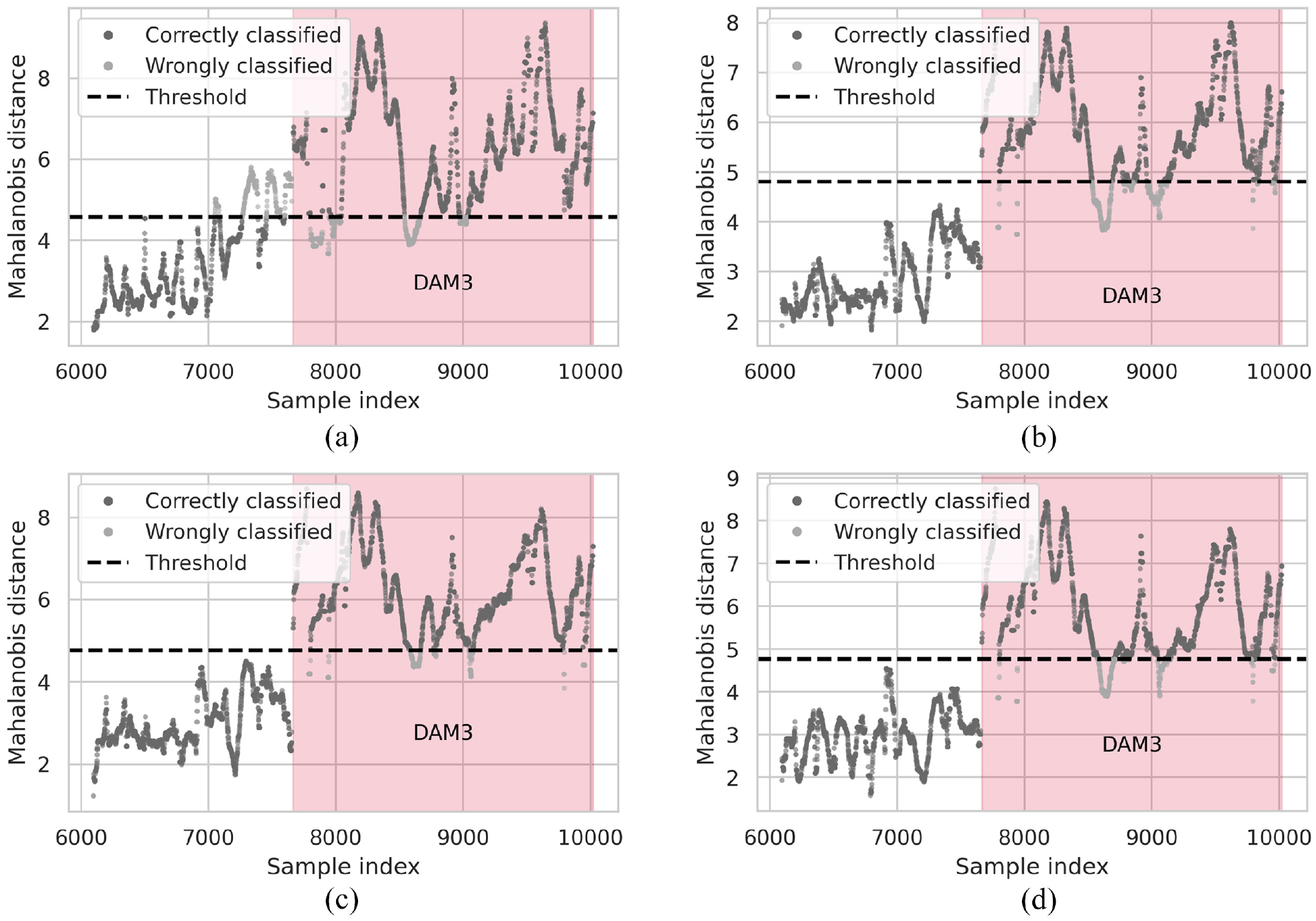
Detectability of DAM3 using 10-min intervals. Again, the different data normalisation approaches and the moving average MD (past 12 h) are considered. The results using the purely data-based GP are shown in (a)
Figure 15(a) shows that data normalisation using a purely data-based GP again does not work reliably, as the threshold is exceeded before DAM3 has been activated. The two grey-box approaches (cf. Figure 15(b) and (c)) demonstrate the capacity to distinguish between the healthy and damaged states with considerable efficacy. In the case of the grey-box model
Evaluation of classification performance encompassing all healthy and damaged states.
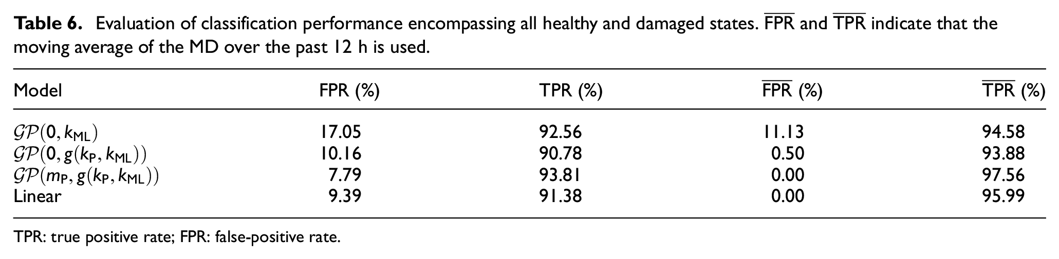
TPR: true positive rate; FPR: false-positive rate.
The results from Table 6 indicate that the grey-box model
To also judge the accuracy of models individually, Table 7 shows the FPRs and TPRs for each of the three healthy respectively repair states and the three damaged states.
Classification of the correct state, considering the three healthy and the three damaged states separately.
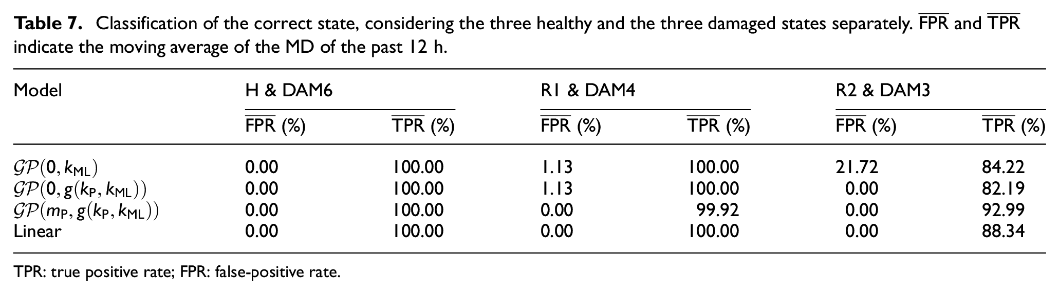
TPR: true positive rate; FPR: false-positive rate.
Table 7 and Figure 15 illustrate that the FPRs und TPRs of all considered models improve for the damage instance DAM3. Therefore, it can be noted that in the case of the 10-min intervals, the quality of the data, especially the precise identification of natural frequencies, significantly impacted the model’s accuracy. However, it is crucial to emphasise that a trade-off is constantly being made. While longer time intervals result in lower uncertainties, this is accompanied by an increasing violation of the underlying system identification assumption of linear time invariance. Consequently, enhancing the data quality by employing longer time intervals is not straightforward and is structure dependent. While higher evaluation times only slightly violate the assumptions for a lattice tower, the assumptions can be much more severely violated for wind turbines due to changes in the rotor speed, for example.
As noted within the previous sections, temperature variations most likely cause the main variations in the natural frequencies. Therefore, the linear model can explain these variations well based on the more accurate identification results. However, the slightly poorer performance of the linear model compared to the grey-box model
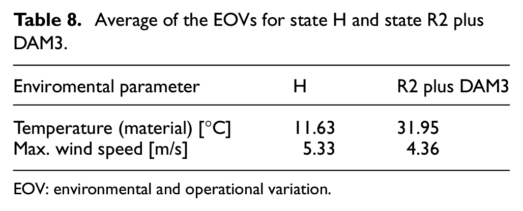
With all models, it is also noticeable that the FPRs are relatively high if no moving average of the MD is used. One reason is the notable disparity in the EOVs contained in the training set with reference to the states R2 and DAM3, as depicted in Table 8.
Average of the EOVs for state H and state R2 plus DAM3.
EOV: environmental and operational variation.
Table 8 highlights a significant discrepancy in the EOV coverage between state H and state R2 with DAM3, particularly concerning material temperature. The findings above show that the purely data-based model is not robust enough to deal with the temperature changes expected from climate change. It is important to note that the grey-box models show an increasing dependency on their white-box components if the EOV coverage in the training data is incomplete. Given that this white-box model describes a linear relationship, the accuracy of the grey-box model converges towards that of the linear model. The extent to which grey-box models depend on their white-box components varies depending on the type of grey-box model utilised.
In terms of the overall performance throughout this study, the grey-box model
Conclusion and outlook
This work compares two novel data normalisation approaches that utilise grey-box methods to account for variations in natural frequencies resulting from changing EOVs that were not included in the training data. Considering such influences in the context of SHM is crucial, as they can cause significant deviations in the dynamic response of structures and mask damage-induced deviations. This is particularly important in the context of climate change, where temperatures are expected to rise. This study addressed this issue by enhancing regression-based data normalisation with machine learning methods. However, machine learning approaches are limited in making meaningful predictions when the new data contains EOVs that were not included in the training set. With this issue in mind, this study’s unique contribution is the application of two grey-box enhanced data normalisation approaches using GP to guarantee plausible mean predictions in the case of unknown EOV regimes due to climate change, their utilisation for subsequent damage detection, and a comparison with a purely data-based GP. Two approaches were employed to integrate the physically plausible linear dependency between the EOVs and natural frequencies into the GP. First, a linear correlation involving the enviromental parameter wind speed and material temperature was encoded through the kernel of the GP. Second, the linear correlation specific to material temperature was incorporated via the GP’s prior mean, and the wind speed correlation was modelled using a combined kernel.
In the case of incomplete training data in terms of poor EOV coverage, it has been shown that the grey-box models capture the underlying trend better than the black-box counterpart, whereby the grey-box model
Grey-box models are a promising approach for a resilient SHM system that can cope with the impact of climate change. However, this requires good modelling of the temperature effects in the case of unknown EOVs.
The damage detection was conducted using the MD. Here, using a moving average of the normalised MD proved advantageous for damage detection, as opposed to using a single data point. Additionally, the predictions were corrected to address the repair problem using an offset
In summary, a grey-box approach, where some dependencies are incorporated as prior knowledge while others are extracted from the data, is beneficial for data normalisation. However, this is only true if the assumed physical mean is correct for unseen conditions. Combining this procedure with the MD for long-term SHM makes it possible to detect the complete removal of one bracing at different locations from the LUMO structure. Here, the grey-box model
Regarding LUMO, the proposed approaches to grey-box modelling showed varying degrees of success, opening up several opportunities for improvement and further development in future work. As previously stated, the correlation to be captured in this study was mainly linear. Therefore, the potential benefits of grey-box modelling approaches to deal with effects related to climate change have only been partially demonstrated. This opens up the possibility of further investigating the robustness of grey-box models to the effects of climate change in the long-term SHM of more complex structures such as bridges or wind turbines. As non-linear effects are expected for these structures, a key challenge is how prior knowledge about these relationships can be incorporated into the grey-box model. In the case of unknown EOV regimes due to climate change, it should also be investigated how frequently new combinations of EOVs arise and how to account for these. As new EOV clusters are formed that differ significantly from the EOV clusters of the training data, handling them in data normalisation is particularly challenging. This is because homogeneous regions in otherwise heterogeneous data are formed. In this case, local cluster-based methods (e.g., local PCA or local multivariate linear regression) could be preferable to global methods. Of particular research interest is how many points from the neighbourhood of a query point have to be included in the prediction in the case of sparse and incomplete training data. Introducing additional forms of prior knowledge could also be beneficial. A case in point is ensuring that the prediction fulfils certain boundary conditions. Moreover, this study did not consider the potential limitations of the predictive variance of GP. The application of heteroscedastic GPs could be particularly suited to mapping these variables with greater precision, whereby the assumption of an underlying normal distribution of variances could also be relaxed. Applying a damage metric that incorporates both the uncertainties from the prediction of the GP and the uncertainties associated with the identification to obtain a probability-based metric appears attractive in this context. Finally, further investigation is required to ascertain the extent of damage that can be reliably detected using different damage detection methods under the effects of climate change.
Footnotes
Declaration of conflicting interests
The author(s) declared no potential conflicts of interest with respect to the research, authorship, and/or publication of this article.
Funding
The author(s) disclosed receipt of the following financial support for the research, authorship, and/or publication of this article: The authors gratefully acknowledge the financial support provided by the Deutsche Forschungsgemeinschaft (DFG, German Research Foundation) – Subproject C02, ID 434502799, SFB 1463.