
Abstract
Data scarcity, coupled with environmental and operational variabilities (EOVs), poses substantial challenges to the generalisability and robustness of damage diagnostic methods for complex components such as wind turbine blades. This paper introduces a novel methodology, termed UCTRF, designed to tackle these challenges. UCTRF stands for Uniform manifold approximation and projection for dimensionality reduction, Capsule neural networks for advanced feature recognition, Transfer adaptive boosting for effective knowledge transfer, and Random Forest for nuanced instance weighting and classification. The UCTRF framework is uniquely suited to scenarios where feature distributions shift due to temperature variations, enabling robust knowledge transfer even in limited datasets. This innovative framework was rigorously evaluated on various temperature-affected datasets, achieving a 95% detection rate. These results underscore its effectiveness in preserving the structural integrity of wind turbines under challenging EOVs and constrained data availability. Additionally, the internal mechanism of the designed domain adaptation captures the alterations in instance weights between the source and target domains during the adjustment process, which can be utilised to analyse the impact of diverse instances on model performance and further refine the adaptation process.
Introduction
The technological shift known as Industry 4.0 has been driving companies towards a lasting transformation of their traditional approaches to production and maintenance activities in recent years. This change encompasses the progressive digitalisation and automation of manufacturing processes, utilising a range of innovative technologies to oversee operations at every stage, from production and management to service and maintenance. 1 Data history from damaged structures is often limited, 2 posing a significant challenge in structural health monitoring (SHM) for complex structures like wind turbines (WTs). 3 This limitation frequently results in overfitting when applying machine learning (ML)-based intelligent damage diagnosis algorithms to these structures.4–8
To address this challenge, one promising approach is the utilisation of simulated data, which can be derived from analytical, numerical or laboratory-based models, and then combined with real-world data from similar machines to train a comprehensive data model. 9 However, the use of simulated data produced by modelling has its own set of constraints such as shifts in the data distribution; this discrepancy may reduce model generalisability and necessitate advanced domain adaptation techniques. For complex structures like wind turbine blades (WTBs), the mathematical modelling step can be intricate and difficult, involving a wide range of parameters from design curves on the structure’s surface to the aerodynamic effects around it. As an alternative, experimental data, either generated in laboratories or captured from other similar machines, can be more beneficial.
Additionally, environmental factors such as temperature fluctuations can affect the stiffness of structures like WTBs, modifying their boundary conditions and influencing their dynamic properties10,11; these changes also affect data collected by sensitive instruments such as piezoelectric sensors, due to their temperature sensitivity. Such variations can result in signal inconsistencies, even when the health conditions remain unchanged, thereby introducing ambiguities in damage detection outcomes. 12
To counter the adverse effects of environmental and operational variabilities (EOVs) in SHM, researchers have developed various techniques, with transfer learning (TL) being one of the most recent advancements. TL capitalises on knowledge from well-established (source) domains to enhance performance in new, related (target) domains, effectively addressing the issue of differing data distributions. A specific form of TL, domain adaptation, focuses on modifying models to bridge these distributional differences, which is especially beneficial when labelled data in the target domain are limited. This approach significantly enhances the predictive accuracy of AI models by adapting to variations arising from factors such as measurement inconsistencies and EOVs.13,14 Each of these types can further be classified within one of three methodological frameworks: feature-based, instance-based or parameter-based approaches.14,15
Main contributions
Given the limitations of current SHM techniques in handling data scarcity and EOVs, this paper presents an innovative framework that combines uniform manifold approximation and projection (UMAP), CapsNets and TrAdaBoost with random forest to enhance domain adaptation under constrained training data and uncertainties from temperature-induced variations, which often disrupt ML-based damage detection. This approach significantly advances SHM methodologies for WTBs. The key contributions of this research are as follows:
A robust SHM framework that adapts to temperature changes.
Integration of advanced feature engineering and ML techniques to handle limited and diverse datasets.
A comprehensive evaluation showing a 95% detection rate on temperature-affected datasets.
The innovation of UCTRF is attributed to its distinctive combination of advanced techniques, namely UMAP for dimensionality reduction, CapsNet for hierarchical feature extraction and TrAdaBoost for domain adaptation, meticulously crafted to tackle cross-domain challenges in WTB damage diagnosis under diverse environmental and operational conditions. This integration uniquely addresses longstanding issues of data scarcity and distribution shifts. UMAP separates complex vibration signals into distinct clusters, improving the interpretability of domain adaptation through TrAdaBoost. Furthermore, CapsNet delivers robust hierarchical feature recognition, and its combination with the adaptive weighting mechanism of TrAdaBoost excels even with minimal training data. This cohesive framework demonstrates exceptional detection rates across temperature-affected datasets, significantly outperforming individual methods. Such integration retains structural insights during dimensionality reduction and enhances the model’s adaptability to unseen data, marking a pivotal development in SHM.
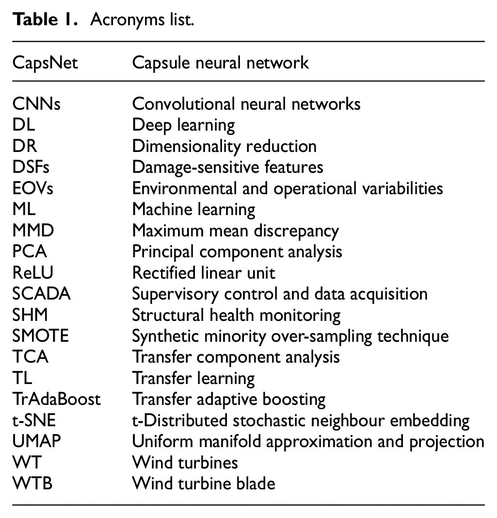
Table 1 summarises the acronyms used in this paper, ensuring clarity and consistency in the technical discussion that follows.
Acronyms list.
The subsequent sections of the paper are organised as follows. A review of the related works is presented in the section ‘Related works’. Section ‘The proposed method’ provides a comprehensive explanation of the proposed approach, encompassing the problem statement, DR, feature extraction, TL and classification. In the section ‘Case study,’ the case study is presented, including details about the dataset used for training, and evaluating the proposed method. Next, the section ‘Results and discussion’ presents the results and discussion. Finally, the section ‘Practical considerations and applicability’ serves as the conclusion, highlighting the main achievements of this proposed method.
Related works
Previous research has addressed SHM challenges using various approaches. Movsessian et al. 16 introduced an artificial neural network-based framework for damage detection in WTBs, focusing on neutralising the impact of EOVs on damage-sensitive features (DSFs) implementing a metric derived from the Mahalanobis distance assessed on both synthesised data and a Vestas V27 WT with various damage scenarios. Hu et al. 17 represented a method for SHM of WTBs by studying the dynamic properties of the considered system over 2 years. By employing principal component analysis (PCA) to adjust for temperature effects, they developed a DSF, successfully detecting simulated damage in the turbine’s blade and tower. This approach underscored the potential for effective long-term health monitoring of WTs, even in the presence of EOVs. Xu et al. 18 proposed a time series analysis, Bayesian cointegration to tackle uncertainties resulting from alterations in temperature and wind speed; this manner, advancing from single to multiple variable assessments, integrated various DSFs.
Chandrasekhar et al. 19 evaluated the operational WTBs’ SHM through a framework that utilised Gaussian processes, recognising that WTBs typically shared identical structural properties and experienced the same EOVS. The implemented methodology fundamentally involves learning DSFs in the long term to account for EOVs where the primary disadvantage is the requirement for domain knowledge to pinpoint characteristics in each case study that can counteract the effects of EOVs. Chen et al. 20 used a combination of Inception V3-a convolutional neural networks (CNNs) model and TrAdaBoost, to diagnose WT damages, including blade icing accretion and gear cog belt failures. This model was examined on an extensive dataset of supervisory control and data acquisition (SCADA) data. They discussed issues posed by unbalanced datasets and EOVs by assigning higher weights to the instances from underrepresented classes. However, they did not consider a comprehensive framework that includes various damage scenarios, such as fatigue damages of distinct severities and quantities, competent of effectively training with a limited number of observations. Li et al. 21 developed a model that combines parameter-based TL and a convolutional autoencoder to capture fault characteristics common across WTs in a single farm, utilising SCADA data. This transferred knowledge from the source turbines to a target turbine with sparse data; the model did not explore faults caused by fatigue-based damage.
Soleimani-Babakamali et al. 22 introduced a TL framework designed for defect detection in structures. The methodology employed high-dimensional features and implemented a generative adversarial network architecture. The TL approach demonstrated promise in effectively distinguishing between no-damage and damage cases, as evidenced by its successful application to three diverse target domain datasets. However, the potential influence of EOVs on the results, as a potential source of uncertainty, was not examined in this approach. The challenge of EOVs impacting vibration-based SHM frameworks was resolved by Roberts et al. 23 In their study, multivariate nonlinear regression was applied to correct DSFs extracted from acceleration data, allowing for their effective normalisation to mitigate the influence of EOVs. Both simulated and operational WTB datasets were implemented to demonstrate the enhancement of defect detection through corrected DSFs, particularly when reducing sensor input information although only one type of malfunction (crack) was considered.
Recently, UMAP has been introduced as a dimensionality reduction (DR) toolkit, displaying promising potential as a feature extraction and visualisation technique in the SHM field. UMAP excels in preserving both local and global structures, unlike t-distributed stochastic neighbour embedding (t-SNE) and PCA. It is more scalable and efficient, managing larger datasets with faster runtime. UMAP requires fewer parameters and is easier to tune than t-SNE. 24
Its flexibility and interpretability make it ideal for feature extraction in SHM. To this end, an indirect SHM framework for assessing the condition of bridge-like structures was launched by Cheema et al. 25 Within this skeleton, UMAP and a non-parametric clustering technique were implemented, and significant effectiveness in detecting alterations in the bridge’s integrity was demonstrated. However, what is more important is the fact that the efficiency of the model was contingent upon the passing of the same type of vehicle over the bridge to which the sensor was attached when the model was designed.
Rahbari et al. 26 addressed the challenges of SHM in the aeronautic industry, where damaged data are rare and costly. They combined DR techniques, such as t-SNE and UMAP, with deep learning (DL) networks to enable the clustering of unknown samples. They evaluated it on composite structures using lamb waves. This approach proved to be more effective when using raw signals compared to traditional malfunction indices. Still, it was suggested that a TL approach ought to be executed in the designed SHM framework to be suitable for cases where the training and testing data are coming from dissimilar sources. From the information presented in preceding research, UMAP-driven techniques have not been applied to the assumptions when there are EOVs, various defect scenarios exist, and the source and target domains differ. As a result, a case study is required to assess the capability of this approach in addressing the mentioned challenges whilst competing approaches such as PCA have been extensively assessed in various scenarios.
Traditional neural networks, such as CNNs, suffer from issues like translation invariance and feature loss due to pooling layers, which pass on only maximum or average values, missing crucial data. CapsNets was introduced by Hinton et al. 27 and utilises capsules (e.g. groups of neurons processing vectors and not scalars) to represent different aspects of a feature and its variations (such as viewing angles). Thus, CapsNets overcomes CNNs’ limitations by maintaining complex feature relationships and improving recognition capabilities. 28
Liang et al. 29 developed a CapsNet-based process for identifying WT gearbox faults. Huang et al. 30 also mitigated the challenge of machinery, that is, automobile transmission health diagnosis under changing working conditions; they launched a weight-shared capsule network for intelligent fault diagnosis of machinery. Although a variety of feature extraction techniques have been applied to the damage detection of WTBs, the potential of CapsNets remains largely unexplored in this field. CapsNets have demonstrated promising results in fault detection within systems similar to WTBs, emphasising their potential applicability in this area. Their unique ability to capture and preserve complex feature hierarchies, alongside accurately recognising patterns under diverse conditions, positions them as a valuable yet underutilised tool for enhancing the diagnosis of WTB malfunctions. This technique offers an improved capability to capture invariant features while maintaining local class-wise separation.
It is noteworthy to acknowledge the dearth of a reliable and generalised technique for diagnosing damage in WTBs, in the face of severe data scarcity in the training observations. This scarcity is exacerbated when dealing with alterations in the data distribution resulting from EOVs and the presence of multiple damage scenarios with varying severity and quantity. Furthermore, it is essential to investigate the use of vibration data in its raw form, rather than transforming it into visual aspects like images that are applied in CNN-based methods, which can be computationally intensive. Determining the best way to convert numerical data into visual formats for use in CNNs presents its own set of challenges. To resolve these concerns, UCTRF a combination of UMAP, CapsNets, TrAdaBoost and random forest was introduced in this work.
First, UMAP was employed to separate observations of various classes in both the source and target domains, facilitating clearer distinctions and improved handling of high-dimensional data. This separation is crucial for enhancing the effectiveness of instance-based domain adaptation methods by simplifying complex vibration signals into more interpretable features. Following this, while maintaining the separation achieved by UMAP, CapsNets positioned some observations from the source domain in close proximity to those in the target domain. This strategic placement allows these selected source domain observations to be reweighted appropriately for domain adaptation, thereby enhancing the adaptation process by bridging the gap between the source and target domain features.
Thirdly, the transferable adaptive boosting, that is, TrAdaBoost component further enhances the model’s ability to adapt to new, unseen data distributions, thereby improving its robustness and generalisability. This constructive interaction between UMAP, CapsNets and TL enables the proposed manner, for example, UCTRF to effectively resolve the challenges of limited training data, varying temperature conditions, and the need for robust feature extraction and classification. Unlike previous approaches, this framework uniquely integrates the DR capabilities of UMAP, the hierarchical feature extraction of CapsNets and the adaptability of TL, enabling precise damage detection even when damage severities are closely similar. This novel combination not only improves the model’s performance across diverse conditions but also offers a more efficient and accurate solution for learning from limited data compared to traditional techniques.
The proposed method
The proposed method (UCTRF) comprises a framework for WTB damage detection under the effect of EOVs alongside limited data for the training procedure (using vibration signals). To achieve this, the dimensionality of raw vibration signals was initially reduced using UMAP, which assists in uncovering the local patterns among various observations within each health scenario, preserving the topological structure of the data and systematically revealing relationships between instances from dissimilar health scenarios. Subsequently, a CapsNet was performed to complete the feature extraction phase; within the CapsNet, various levels known as capsules detect and encode diverse characteristics of an observation. Initial capsules are designed to recognise simple patterns such as sudden changes in amplitude, whilst the higher-level capsules are well-positioned to discern complex phenomena, including harmonic frequencies or modulations that each mechanical fault can reveal. This advancement is specifically engineered to detect and delineate spatial and hierarchical subtleties across non-identical instances of damage conditions. The final layer of the CapsNets, namely the classification layer, is removed, and the features extracted from the ultimate capsule are flattened (transformed into a vector format) to ensure compatibility with subsequent processing stages. It is noteworthy that the sequential application of UMAP and CapsNet achieves a more comprehensive data representation as demonstrated by scatter plots later in this work.
Domain adaptation and classification were subsequently achieved using TrAdaBoost, with random forests chosen as the classifier to mitigate the adverse effects of EOVs; the primary components of UCTRF are outlined as follows: (i) employing UMAP for DR, (ii) extracting features through CapsNets and (iii) adapting to different domains using TrAdaBoost. Figure 1 summarises the procedure of malfunction classification in a WTB for UCTRF.
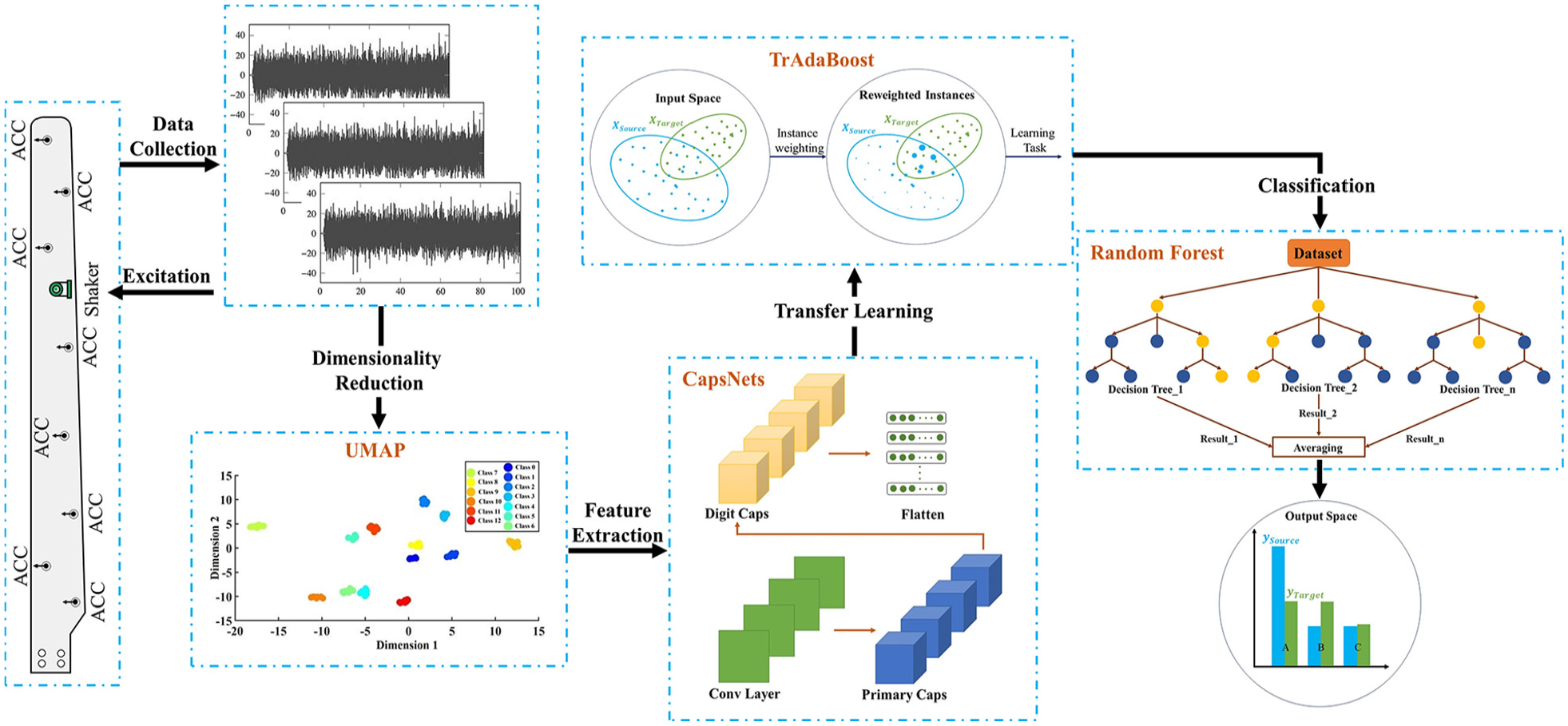
Wind turbine fault classification framework of UCTRF.
Dimensionality reduction
DR assists in isolating noteworthy features from data, enhancing the efficiency and accuracy of fault diagnosis and predictive maintenance models. UMAP, a non-linear technique for DR, seeks to convert complex and high-dimensional data such as vibration responses used in UCTRF into a simpler, low-dimensional Euclidean space. This Euclidean space allows for straightforward distance calculations and geometric interpretations, which facilitate the analysis and visualisation of the vibration signal. UMAP preserves both the detailed and pervasive characteristics of the data. Utilising manifold learning approaches, UMAP operates under the assumption that data points in a high-dimensional vibration signal are evenly spread across local manifolds.
The implemented methodology for DR of vibration signal can be divided into two primary phases: the creation of a high-dimensional topological structure and its subsequent projection into a lower-dimensional space. Assume a vibration signal (
UMAP establishes simplex structures by determining the
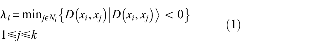
where
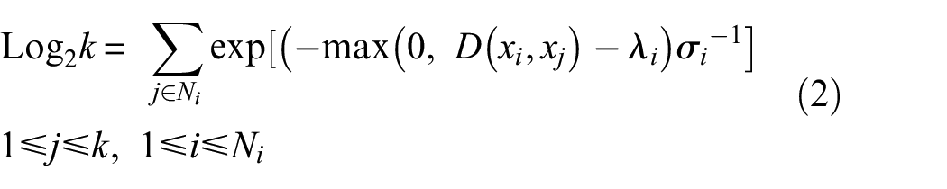
UMAP establishes local fuzzy simplicial memberships in the high-dimensional space,
The first stage goal is to derive an expression of the probability that two points are connected in high dimensions. Objects that are more alike are given a higher probability whilst those that have fewer similarity receive a lower probability; the conditional probability can be expressed as 32 :
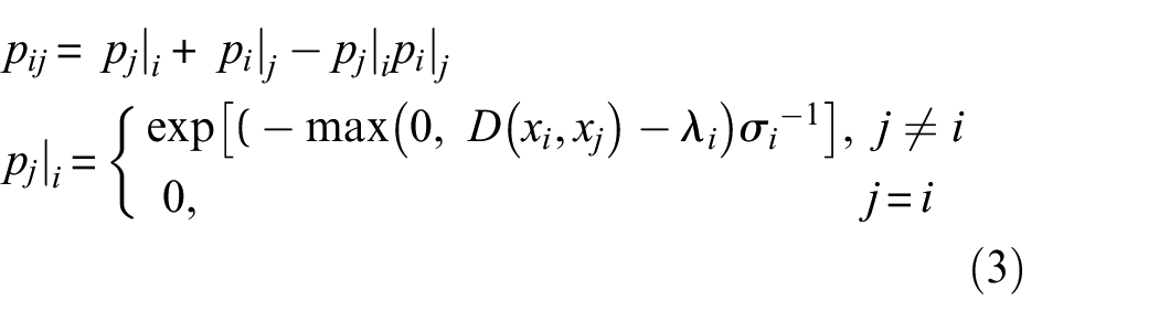
in which
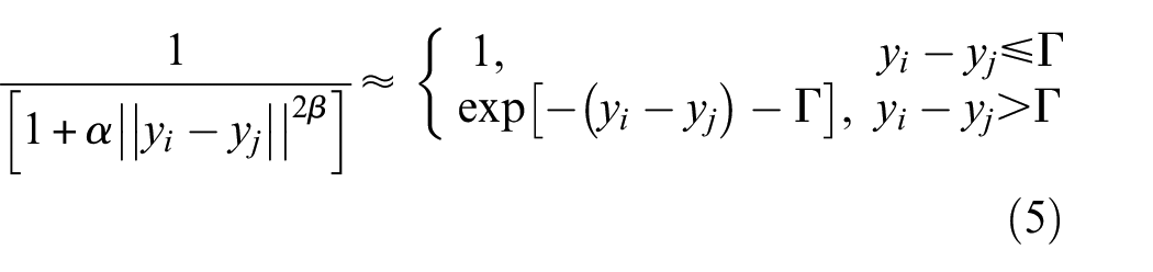
The second stage goal is to project the constructed topology into a visually comprehensible in the embedding
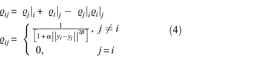
where
‘
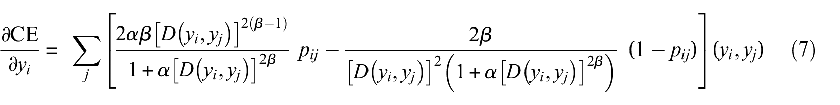
UMAP uses a cross-entropy operation, which clusters or separates data points based on the outputs from the first stage. The cross-entropy function has attractive and repulsive components, where similar points are attracted to each other. This process forms clusters while points with differing features are repulsed, ensuring appropriate separation between clusters. This process is optimised using techniques like negative sampling and stochastic gradient descent, making UMAP more efficient and more effective with high dimensions than t-SNE.
The UMAP performs optimisation while minimising the cross-entropy (CE) between the distribution of points in the original and the embedding spaces31,32:
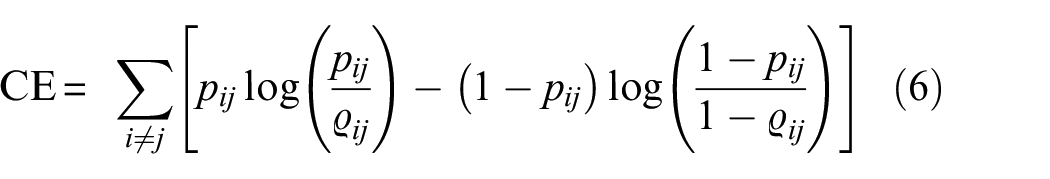
The reduction process begins with a specified initial group of points in the embedded space; UMAP implements the graph Laplacian matrix to determine the starting low-dimensional positions, and then continues the refinement using gradient descent.31,32
After completing the analysis, UMAP provides a final two-dimensional fuzzy graph that retains the underlying data structure of the source signals. The clustering of signals in this graph can be used to analyse similarities and differences in the measured signal features; after completing the optimisation, the final reduced vector (

where
Feature extraction
The ultimate stage of the feature extraction phase of UCTRF utilises an extension of the CapsNets launched by Sabour et al. 35 This network includes convolutional layers for feature extraction, normalised by activation functions like the rectified linear unit (ReLU), followed by a primary capsule layer with multiple capsules converting scalar outputs to vectors, adapting to dataset complexity.
One more benefit of CapsNet is the introduction of the digit capsule layer, which coming after the primary capsule layer and serves dual purposes: identifying the presence of a specific feature and its properties. The layer is shown in Figure 2 which uses the CapsNet framework to refine features from a vibration signal. Initially, the feature vector of an observation is fed into the convolutional layers with dimensions
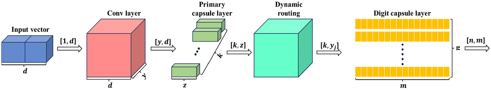
Structure of the designed CapsNets.
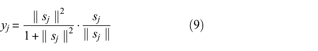
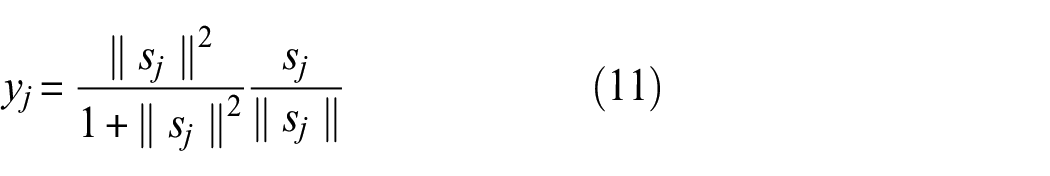
Since the outputs of both the primary and digit layers are vectors, a novel nonlinear activation function, namely ‘squashing’ was implemented to produce the activity vector of the capsules, that is, constrains the output values to be placed between 0 and 1. While it preserves the vector orientation in agreement with the lower-level capsules’ predictions, it also guarantees that the vector norm remains below 1, thereby representing the probability of the presence of the associated entity 36 ; this function can be defined as:
The network employs a ‘routing algorithm,’ which is typically dynamic, to adjust the connection weights between primary and digit capsules according to their output agreement. This dynamic routing replaces the max pooling layer found in CNNs, enabling CapsNet to learn feature hierarchies. By iteratively refining coupling coefficients, dynamic routing ensures that higher-level capsules
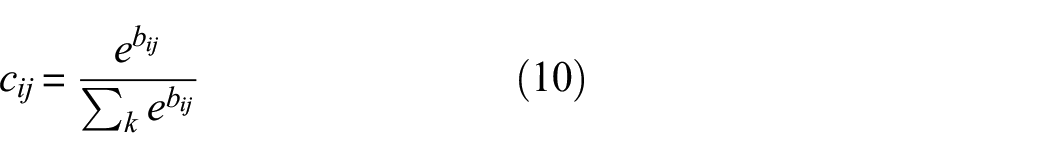
These coefficients quantify the agreement between the predicted output
This procedure normalises the magnitude of capsule outputs to lie between 0 and 1 while preserving their direction. This ensures that the output vector
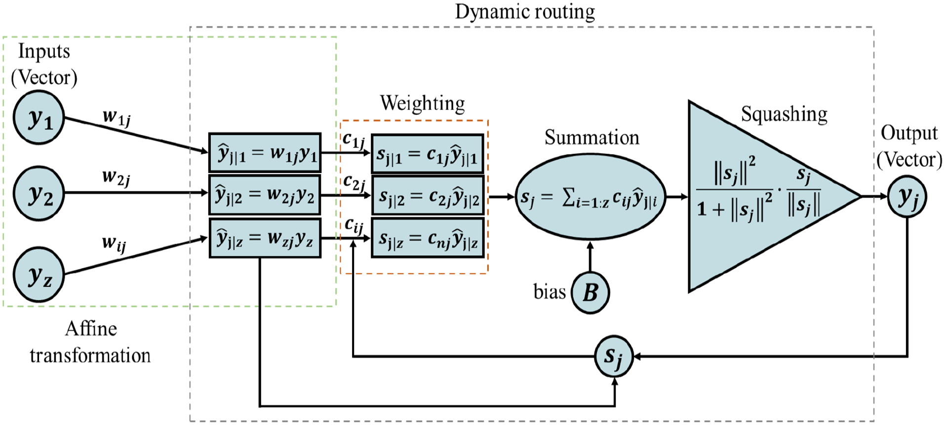
Workflow of a dynamic routing mechanism.
CapsNet often utilise the margin loss function, which relies on three key parameters: the positive constant (m_plus), the negative constant (m_minus) and the weighting factor (Loss_lambda) to ensure accurate predictions. ‘m_plus,’ usually near 1 (e.g. 0.9), sets the minimum output vector length for correct predictions, penalising shorter vectors. ‘m_minus,’ around 0.1, limits the length of incorrect prediction vectors, with excess lengths incurring losses. The ‘loss_lambda’ parameter reduces the impact of incorrect classifications, prioritising correct ones and supporting the network’s learning of part-whole relationships.
From Figure 3,
Removing the output layer of an ML or DL model can transform it into a feature extractor. In this study, the output layer of the CapsNets, originally a SoftMax layer, was removed. Consequently, the output vectors from the digit capsule layer now serve as the feature vectors for each observation.
Transfer learning
TrAdaBoost technique was employed in this work as a tool to mitigate the adverse effects of EOVs, extends the AdaBoost algorithm and serves as the TL framework. This technique enables the development of a high-quality classification model for a novel domain (i.e. target domain) with minimal newly labelled data, particularly when only labelled data from the source domain are available. By operating on a ‘reverse boosting’ principle, the technique adjusts training instance weights iteratively, decreasing the weights of source instances that are poorly predicted while increasing those of target instances. This strategy ensures effective knowledge transfer, delivering accurate results while optimising both time and resources 38 ; the algorithm executes the subsequent steps:
(a) Adjust weight values to a standard scale:
where
(b) Train an estimator ‘
(c) Calculate error vectors for the training samples:


where
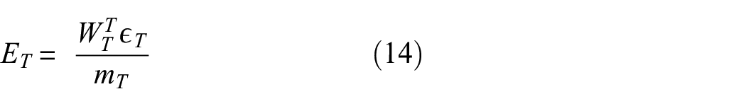
(d) Calculate the overall weighted error for the target samples:
(e) Update source and target weight values:
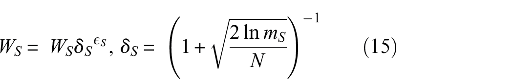

where
(f) Loop back to step ‘a’ and continue until the specified number of boosting iterations
The outcome is determined by considering the results of the last
TradABoost does not depend on a particular type of classifier, so this algorithm can be combined with various classification models, such as ridge classifiers, random forests, support vector machines, neural networks and so on; this flexibility allows one to choose a base classifier that aligns well with the specific challenge being addressed. 39
Classification
Classification is the last step of UCTRF; to this end, random forest was applied as the classifier which is an ensemble approach that is employed not only for classification and regression but also for tasks like feature selection and anomaly detection. During its training, multiple decision trees are constructed. For classification, either a majority vote from the trees is relied upon or their outputs are averaged. Its ensemble approach protects overfitting, and varied data types are effectively processed by it, showcasing resilience to outliers and noise.40,41
In a random forest algorithm, certain hyperparameters ought to be specified such as maximum depth, minimum value of samples split, minimum number of samples leaf, maximum magnitude of features and so forth. A principal parameter is the number of estimators, which denotes the quantity of decision trees within the forest. This parameter determines the count of contributing predictors influencing the model’s final prediction. While an elevated value can enhance prediction accuracy, it simultaneously impacts computational efficiency. Figure 4 illustrates the process of implementing domain adaptation with the TrAdaBoost algorithm, where a random forest classifier is utilised.
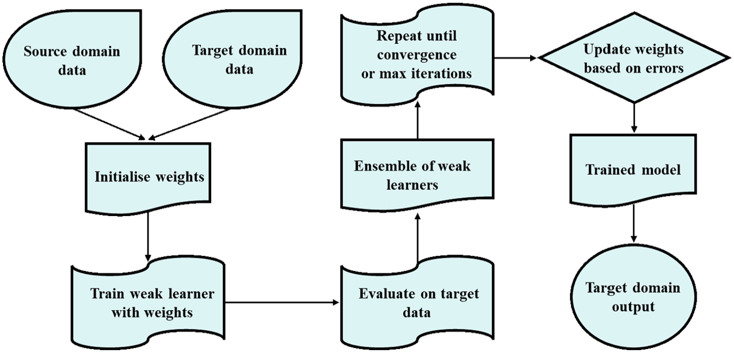
Procedure for domain adaptation with TrAdaBoost and random forest classifier.
Case study
To examine the proposed SHM framework, the dataset disclosed by Qu et al. 42 is considered. This dataset contains experimental vibration signals of a small-scale WTB for the blade of a Windspot 3.5 kW WT model manufactured by Sonkyo Energy (Figure 5); this blade is made of a three-layered sandwich composite configuration; it has a length of 1.75 m and a mass of 5.0 kg. The signals were obtained under disparate health and environmental conditions. Figure 6 shows the schematic of the considered WTB with the locations of the exciting and receiving sensors as well as the faults’ positions. 42
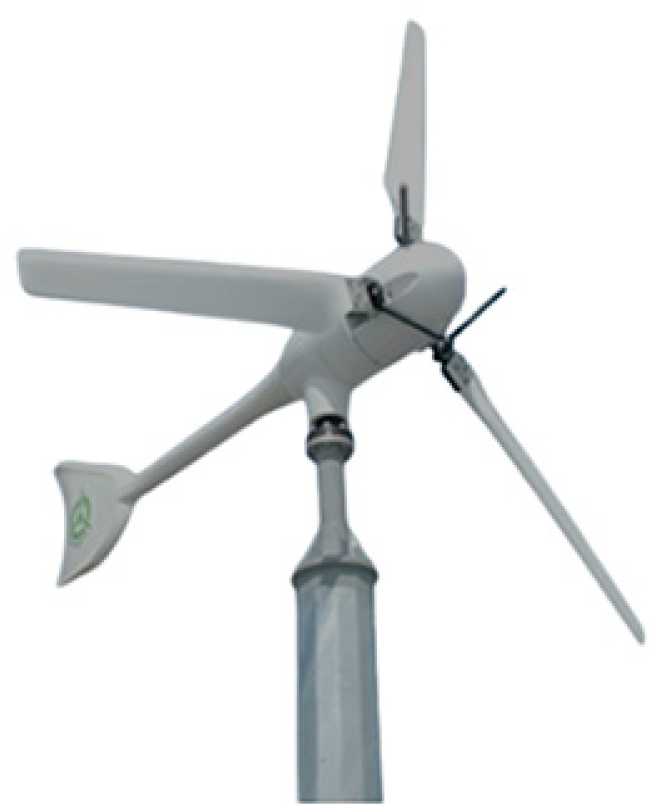
The 3.5 kW WT made by Sonkyo Energy. 42
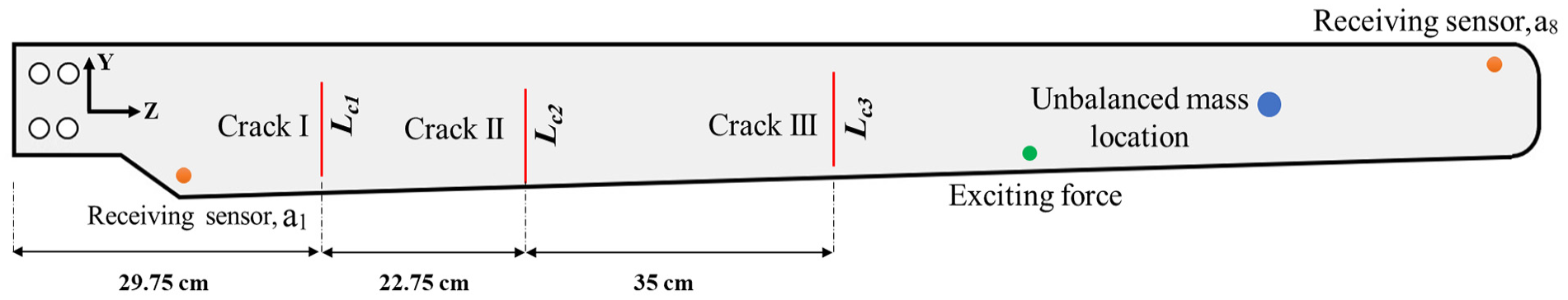
Positioning of the sensors and damages on the investigated WTB.
The experiments were performed under 12 different temperature conditions, ranging from −15 to 40°C with 5° increments in a 60% humidity condition. Two various excitation modes were applied individually: a white noise signal over a 0–400 Hz frequency range, and a sine sweep signal with a frequency range of 1–300 Hz. Both excitation models were applied for approximately 120 s, although the length of the captured signals varied slightly. The crucial aspect is that the sampling frequency remained constant at 1666 Hz. Additionally, the excitation was applied at a fixed point on the surface of the blade, depicted by the green circle as the exciting force in Figure 6. Signals were captured by two distinct types of sensors: a set of accelerometers and a set of strain gauges, with each set configured differently. The physical properties of these installed sensors can be found in Chawla et al. 43
A total of 13 different health scenarios were considered for the WTB. These conditions included one intact state, nine cases with cracks (with varying numbers of cracks ranging from 1 to 3 and different crack lengths) and three scenarios involving icing accretion (achieved by adding unbalanced masses of 44 g in quantities of 1–3). Table 2 summarises these varying health scenarios along with the quantity and the fault severity. It is worth noting that the introduced index will be used later in the classification process.
WT blade health conditions.
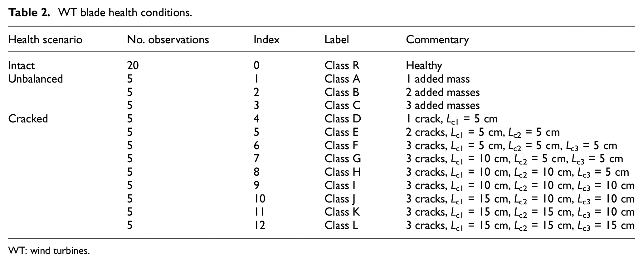
WT: wind turbines.
Results and discussion
In this study, multiple scenarios were examined to showcase the effectiveness of the proposed damage detection framework for the WTB. These scenarios included data augmentation, DR, fault diagnosis without domain adaptation, utilising UCTRF, fault diagnosis applying two other TL methods, that is, domain-adversarial training of neural networks (DANNs) and transfer component analysis (TCA), and adjusting instance weights during the adaptation process. Each of these aspects is thoroughly explored in the subsequent sections.
Data augmentation
In the present work, the collected data by sensors a1 and a8 (Figure 6) were evaluated under diverse temperature conditions. Data corresponding to +5°C were designated as the source domain (training material) whilst data from six alternative temperatures, namely −15°C, −10°C, −05°C, +15°C, +25°C and +35°C were treated as distinct target domains (testing sets). It is important to emphasise that each of these target domains was inspected individually, rather than being consolidated into a singular target domain dataset.
Since the number of observations in the source and target domains is limited, for example, consisting of 20 vibration signals under healthy conditions and 5 signals for each faulted scenario a data augmentation technique, the synthetic minority over-sampling technique (SMOTE), was implemented to increase the number of observations of the damaged WTB from 5 to 20. This strategy augments the minority classes by producing synthetic samples, leveraging interpolation between existing data points. SMOTE identifies a minority class instance and one or more neighbouring instances
The value
In the process of data augmentation, it is essential to introduce sufficient variability to ensure that the generated data are not identical to the original dataset. This would undermine the purpose of augmentation, which seeks to improve model generalisation by introducing diversity. However, a balance must be maintained between the similarity to the original data and the variability introduced. Excessive similarity may restrict the model’s capacity for generalisation, while imprudent variability could result in the synthetic data diverging significantly from the original class characteristics. While alternative generative methods, such as generative adversarial networks 6 and physics-informed models, 44 exist for synthesising data based on probabilistic models, the goal here was not to model probabilistic scenarios but to balance the dataset effectively, making SMOTE a suitable choice.
To evaluate the effectiveness of the SMOTE method implemented for data augmentation, the MMD was calculated for 12 faulty health scenarios and the normal WTB condition. For the healthy condition, two subsets of 5 and 15 samples, both derived from the original dataset, were randomly selected to represent the original and the arbitrary synthesised data. MMD measures the discrepancy between the original and synthesised datasets by comparing their distributions in high-dimensional space, using a kernel function to project and assess the similarity between these distributions. A higher MMD value (greater than 0.1) indicates significant variability between the original and synthesised data, suggesting improved generalisation, though this may reduce separability between classes. Lower MMD values (between 0.01 and 0.1) imply greater similarity, while values below 0.01 suggest that the synthesised data are too similar to the original, which is undesirable for effective augmentation.
The MMD calculation requires the selection of a kernel function; in this study, the Radial Basis Function (RBF) kernel was chosen for its capability to manage high-dimensional data and capture non-linear relationships in the signal data. A gamma value of 1.0 was selected, providing a balance between sensitivity to minor differences and computational efficiency. The flexibility of the RBF kernel allows for a precise assessment of the divergence between the original and synthesised data. The MMD results confirm that the SMOTE technique introduced meaningful variability across the faulty health scenarios without substantial deviation from the original data distributions. Figure 7 presents the computed MMD values for the 13 classes, with −10°C and +35°C as target domains and data collected by sensor a1. The entire process was implemented using Python within Jupyter.
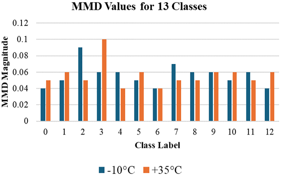
MMD between the original and augmented data for 13 health conditions.
The MMD values observed for both −10°C and 35°C conditions across the 13 classes indicate that the SMOTE-synthesised data successfully strikes an appropriate balance between preserving similarity to the original dataset and introducing sufficient variability for meaningful augmentation. In the case of the healthy condition, where 5 original and 15 synthesised samples were derived from experimental data, MMD values of 0.04 and 0.05, respectively, align with the established threshold range of 0.01–0.1. These values confirm that the synthesised data exhibit the requisite level of diversity without deviating excessively from the original data distribution, thus ensuring that the augmentation process contributes positively to model generalisation. Consequently, this analysis substantiates the effectiveness of the SMOTE approach in maintaining the integrity of class characteristics while enhancing the dataset’s variability, a key factor in improving the robustness and adaptability of the model.
Reducing the dimensionality
Following the augmentation of the dataset through SMOTE, UMAP analysis was conducted on the balanced versions of the source and target domain datasets to diminish the dimension of each vibration signal to 200. To gauge the effectiveness of the UMAP approach, a comparison was made with another widely recognised dimensionality method, that is, PCA. The scatter plots derived from the UMAP and PCA analyses on the source dataset (sensor a1) are depicted in Figure 8(a) and (b), respectively, offering a visual representation of the outcomes.
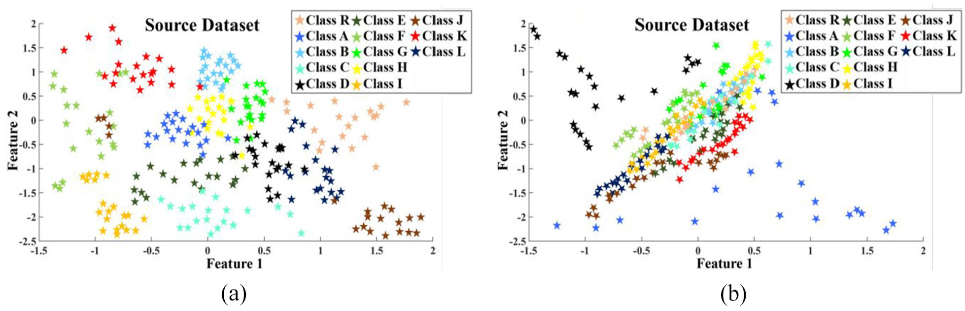
Scatter plot of (a) reduced dimension using UMAP and (b) reduced dimension using PCA.
The plots demonstrate that the UMAP technique (Figure 8(a)) exhibits a superior ability to distinguish between different class observations compared to PCA (Figure 8(b)), as the space reduced by PCA appears denser in certain areas.
To statistically compare the impact of PCA and UMAP, the silhouette score was employed. This metric, ranging from −1 to 1, evaluates the effectiveness of clustering by measuring how similar objects are within the same cluster compared to those in contrary clusters. 45 For the study, the average silhouette score for 13 classes was calculated; scores closer to 1 signify that the clusters are well-defined and separate clearly, which is crucial for ensuring the robustness and reliability of these DR methods in distinguishing and visualising different data classes. UMAP demonstrated a higher clustering capability (mean: 0.5793) in comparison to PCA (mean: −0.3067), highlighting UMAP’s more effective ability to group similar cases for the present application. This comparison is represented through bar graphs that display the average silhouette scores for each class, as depicted in Figure 9.
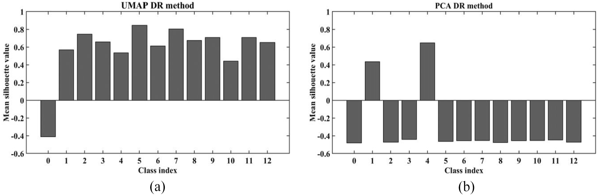
Comparative analysis of clustering performance: (a) UMAP and (b) PCA silhouette scores.
Whilst the implementation of UMAP demonstrated higher performance compared to PCA, as shown in Figure 8(a), one can understand that overlaps between observations of various classes still exist, indicating the need for further feature refinement. To tackle this issue, CapsNets were employed within the reduced dimensionality space provided by UMAP.
Feature refinement through CapsNets
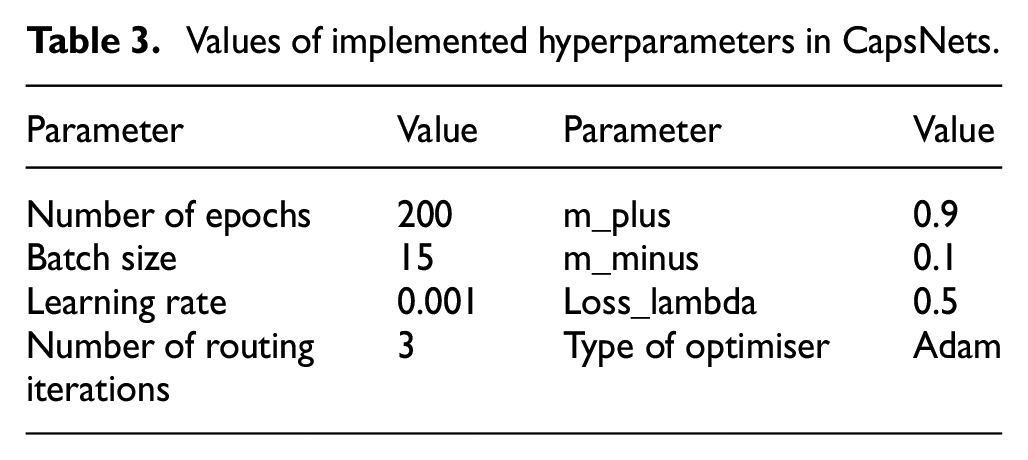
As the ultimate step in feature engineering for UCTRF, CapsNets were applied to the outputs of UMAP. To achieve this, a set of hyperparameters, detailed in Table 3, were assigned; scatter plots in Figure 10(a) and (b) illustrate the data distribution generated by CapsNets for both the source and target domain data (collected at −15°C) for sensor a1. A thorough process of manual trial and error was carried out to optimise the values of the specified hyperparameters.
Values of implemented hyperparameters in CapsNets.
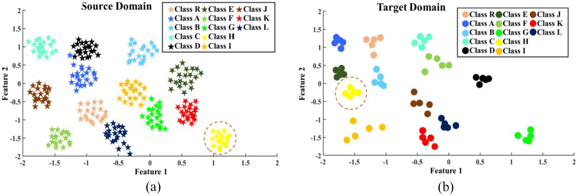
Scatter plot of (a) source domain observations and (b) target domain observations.
From Figure 10, it can be seen that the regions occupied by observations of various classes have changed between the two domains. As an illustration, one can notice the shift in regions associated with class H observations (yellow-colour shapes surrounded by the red dashed circle). Consequently, the network trained on samples from the source domain struggled to correctly identify observations from the target domain.
Classification without the TL algorithm
To present the adversarial effects of the EOVs in the damage detection task, the entire algorithm was initially run without TrAdaBoost for damage classification. In this procedure, the algorithm, which consists of UMAP, CapsNets and a random forest classifier, was trained using source domain data (observations recorded at +05°C through sensors a1 and a8). It was then evaluated on samples derived from signals captured at −15°C (recorded by the same sensor). It is worth noting that, when utilising TrAdaBoost, 15 instances from each class were allocated randomly for the domain adaptation stage, with the remaining five observations from each class designated as testing material; the confusion matrix for the test phase is presented in Figure 11(a) and (b) for sensors a1 and a8, respectively. Furthermore, the number of estimators and the amplitude of the learning rate of the classifier were regulated at 20 and 0.1, in order.
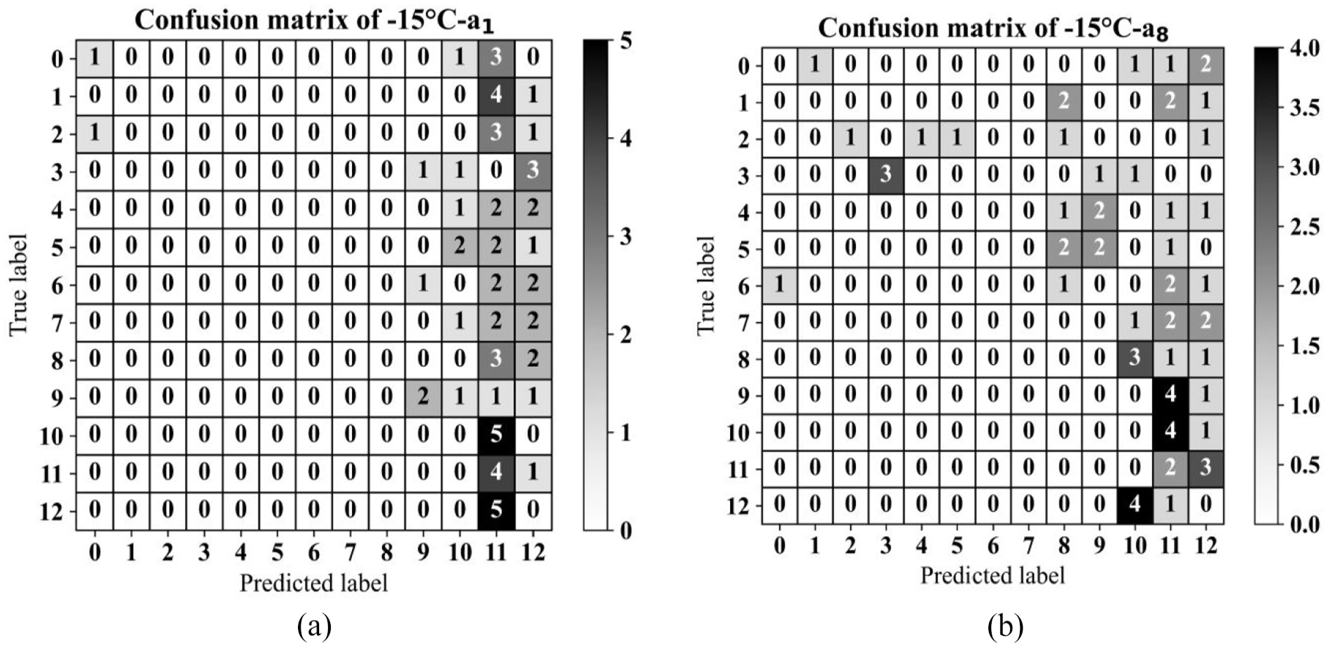
Confusion matrix of the test phase (−15°C) of the classification algorithm without TL (a) sensor a1 and (b) sensor a8.
From the plotted confusion matrices, it can be observed that the classification model without TL struggled to accurately classify observations from various domains based on the severity and type of failures, achieving an accuracy rate of approximately 11% for sensor a1 and 9% for sensors a1 and a8, respectively.
Classification using UCTRF
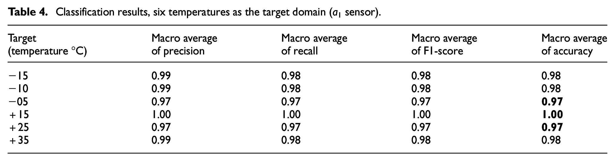
This section discusses the training of UCTRF using enhanced data from +05°C as the source domain, with samples from other temperatures acting as the target domain. It should be noted that this approach was applied separately to sensors a1 and a8. The average evaluation metrics for these sensors are provided in Table 4 (for a1) and Table 5 (for a8), where the minimum and maximum accuracies achieved are highlighted in bold. Furthermore, the framework’s effectiveness in damage detection, that is, measured by the F1 score across all damage scenarios and target domain conditions, is illustrated in Figure 12(a) for sensor a1 and Figure 12(b) for sensor a8. As previously mentioned, for each target domain scenario, 15 samples were allocated to the TL process, including training and validation phases, whilst the remaining five samples were designated for testing.
Classification results, six temperatures as the target domain (a1 sensor).
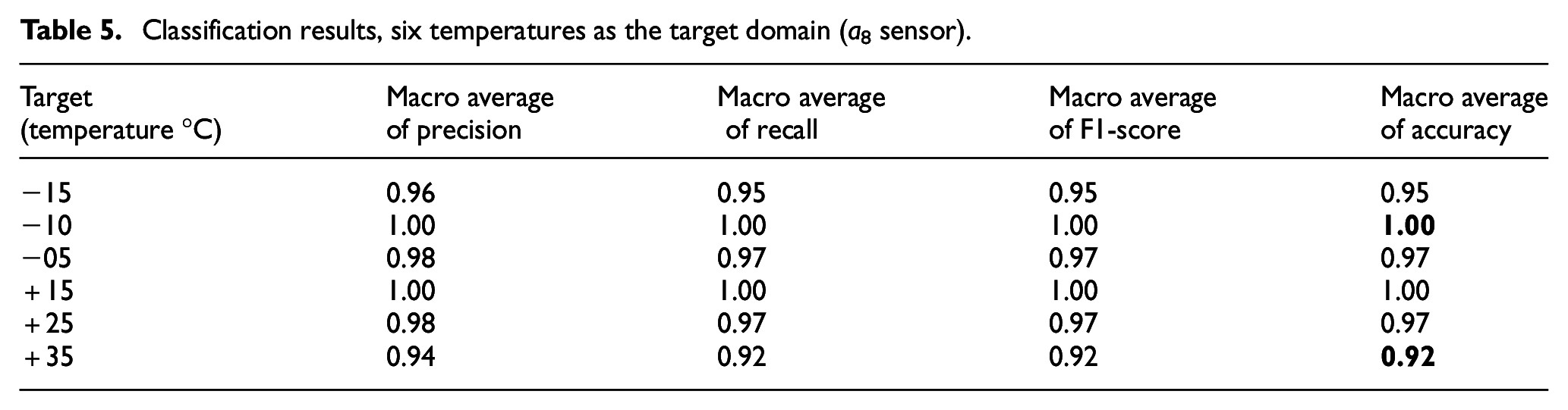
Classification results, six temperatures as the target domain (a8 sensor).
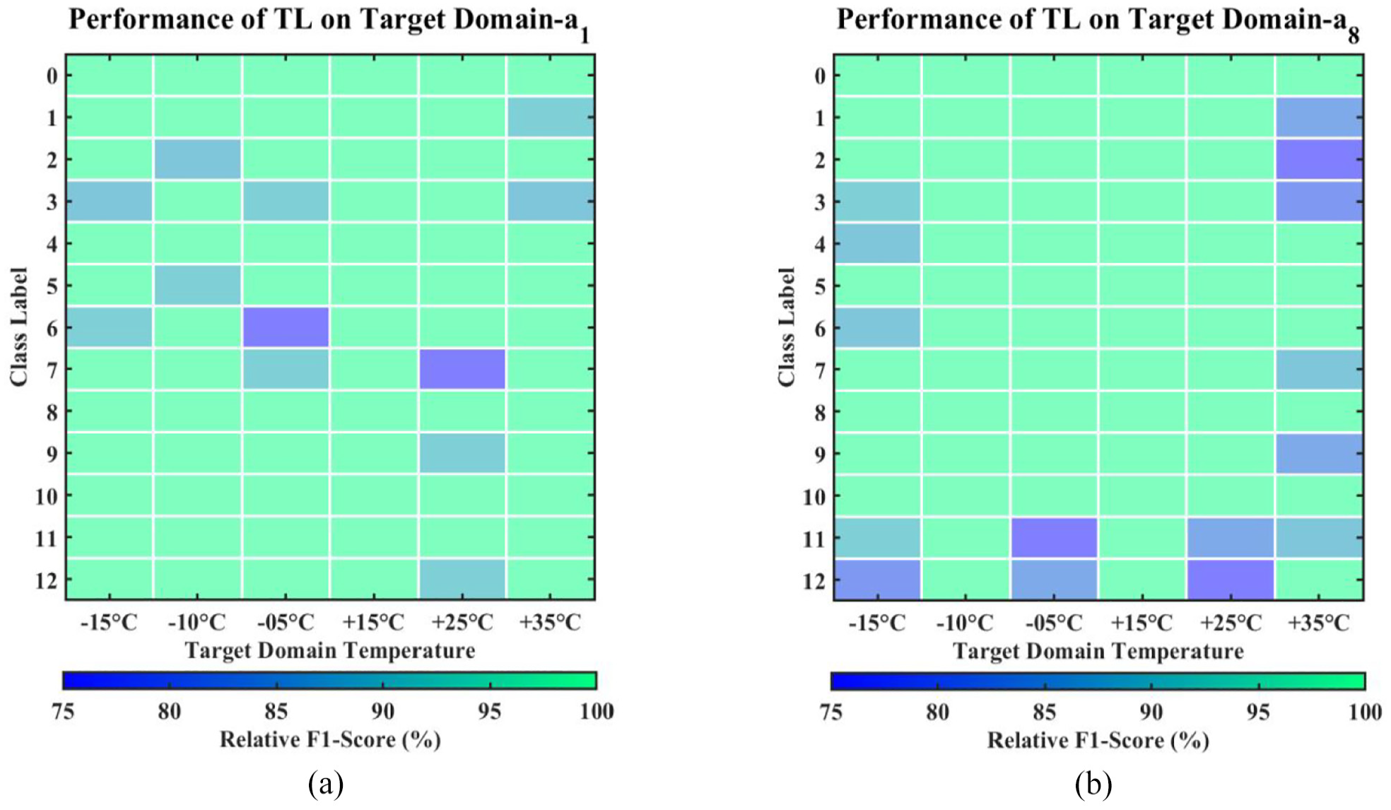
Efficacy of UCTRF across all temperatures and damage types for (a) sensor a1 and (b) sensor a8.
From Figure 12 and Tables 4 and 5, it can be observed that the a1 sensor consistently demonstrated superior performance, with macro average precision, recall, F1-score and accuracy well above 0.95 for all temperature levels. Notably, for extremely cold temperatures of −15°C and −10°C, the model achieved precision and recall above 0.99, along with an F1-score and accuracy of 0.98. The model’s performance remained consistently high for moderately cold temperatures of −5°C and mildly hot temperatures of +25°C, with all metrics exceeding 0.97. Impressively, the model achieved perfect scores across all evaluation metrics for extremely hot temperatures of +15°C and +35°C. It is noteworthy that the mentioned results were achieved when only 20 observations for each class were employed as the training ingredient. On the other hand, the a8 sensor, although performing well, showed slightly lower performance in temperature classification, particularly for the most extreme conditions of −15°C and +35°C. These findings highlight the variations in classification performance specific to each sensor and underscore the a1 sensor’s strengths in accurately predicting temperature levels across diverse environmental conditions.
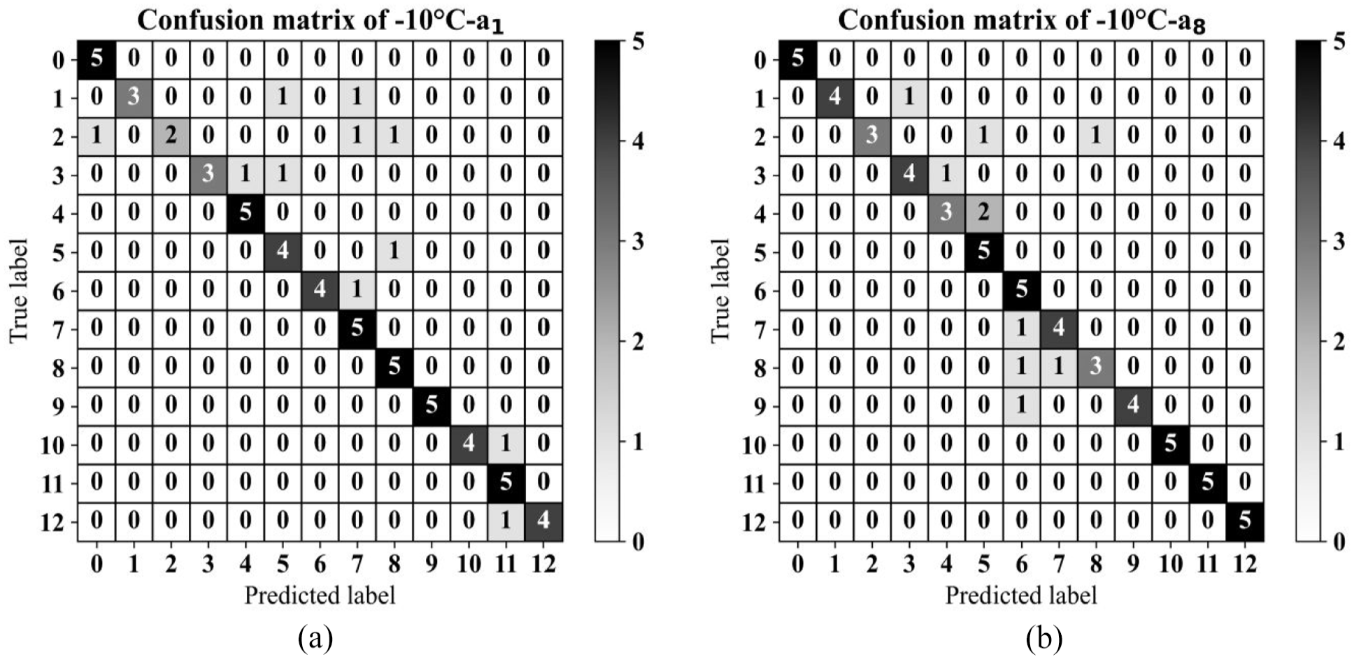
The confusion matrices for two distinct temperature scenarios, −10°C and +35°C, are illustrated in Figure 13(a) and (b) for sensor a1. Using data from sensor a1, of the 65 test phase observations, only one was inaccurately classified, mistaking an unbalanced scenario sample for a cracked WTB sample. In a similar vein, sensor a8 accurately classified 98.46% of its observations. However, there was one instance where a severely unbalanced WTB sample (labelled as class 3) was erroneously identified as a slightly unbalanced scenario (labelled as class 1).
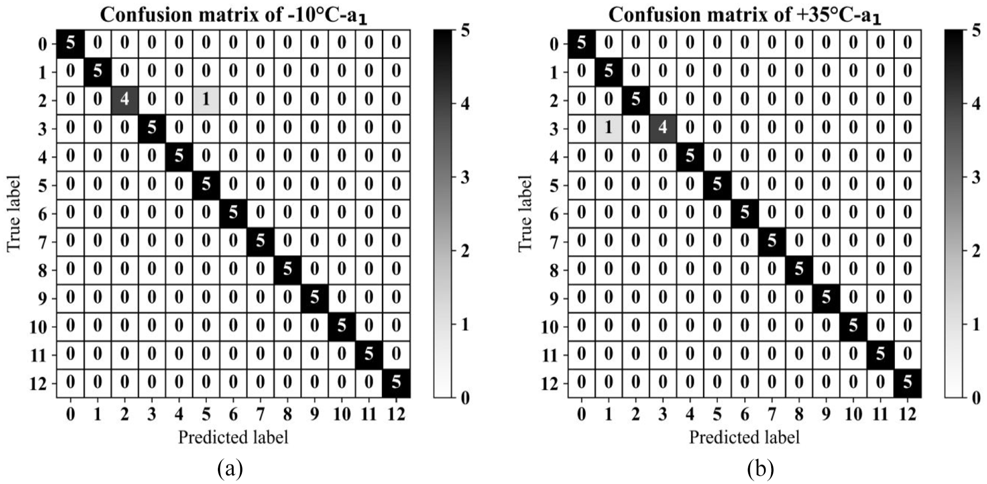
Confusion matrices for data collected using the a1 sensor during the testing phase of UCTRF, with source domain at +5°C: (a) target domain at −10°C and (b) and target domain at +35°C.
Similarly, the confusion matrices of the two temperature scenarios at −10°C and +35°C are plotted for a8 in Figure 14(a) and (b), respectively. The results at −10°C demonstrate remarkable accuracy, with 100% of observations correctly classified. Conversely, the classification performance at +35°C was comparatively lower at 92.31%. In this scenario, out of the observations assigned to the class labelled as 2, five were incorrectly classified.
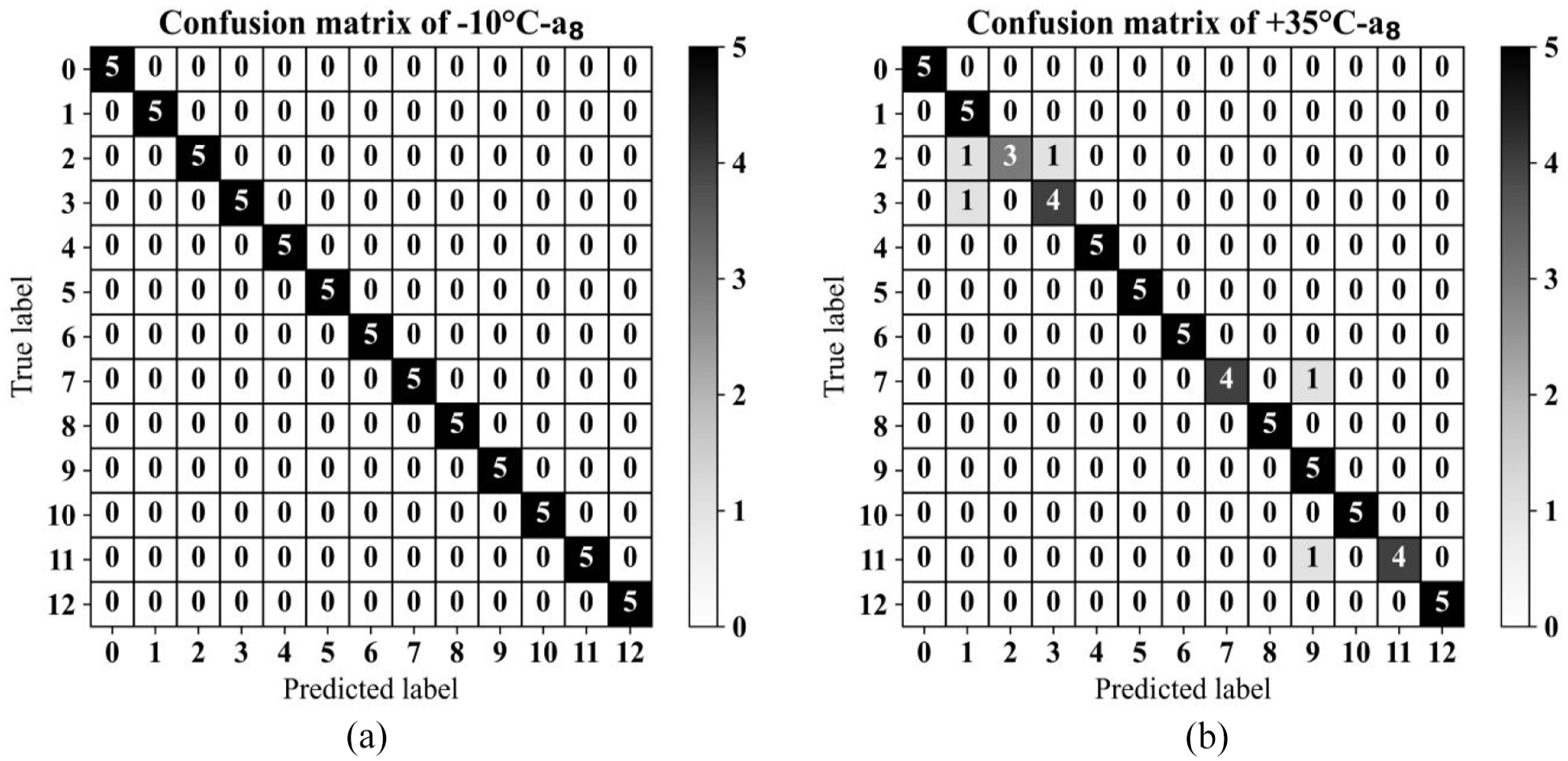
Confusion matrices for data collected using the a8 sensor during the testing phase of UCTRF, with source domain at +5°C: (a) target domain at −10°C and (b) and target domain at +35°C.
The varying classification results from sensors a1 and a8 can be largely attributed to the distinct training processes of their respective TL models. The training of each sensor’s model was independently conducted utilising source domain data, followed by individual evaluations on target data that represented a range of temperature conditions. These disparities in training data and the adjustment of the models are significant determinants of the fluctuations in classification efficacy.
The a1 sensor, strategically positioned closer to the WTB’s base, procured vibration signals likely to contain a higher quota of pertinent structural data, even in the context of an experimental environment. Therefore, the model educated by the a1 sensor data acquired characteristics and patterns exceptionally responsive to temperature-related alterations, leading to a consistently elevated classification performance.
By contrast, the a8 sensor, situated at a greater distance from the base, registered vibration signals that were impacted by different sections of the blade and the materials used, potentially obstructing the model’s capacity to generalise accurately to the target temperatures. The variances in the training data coupled with the sensor’s relative location to the structure of the blade are probable contributors to the marginally diminished classification precision of the a8 sensor model, particularly under severe temperature conditions. To encapsulate, the disparities in classification outcomes are rooted in the singular training experiences specific to each sensor, underlining the influence of sensor placement and training data on a model’s ability to classify temperatures in a controlled setting.
Classification using DANN
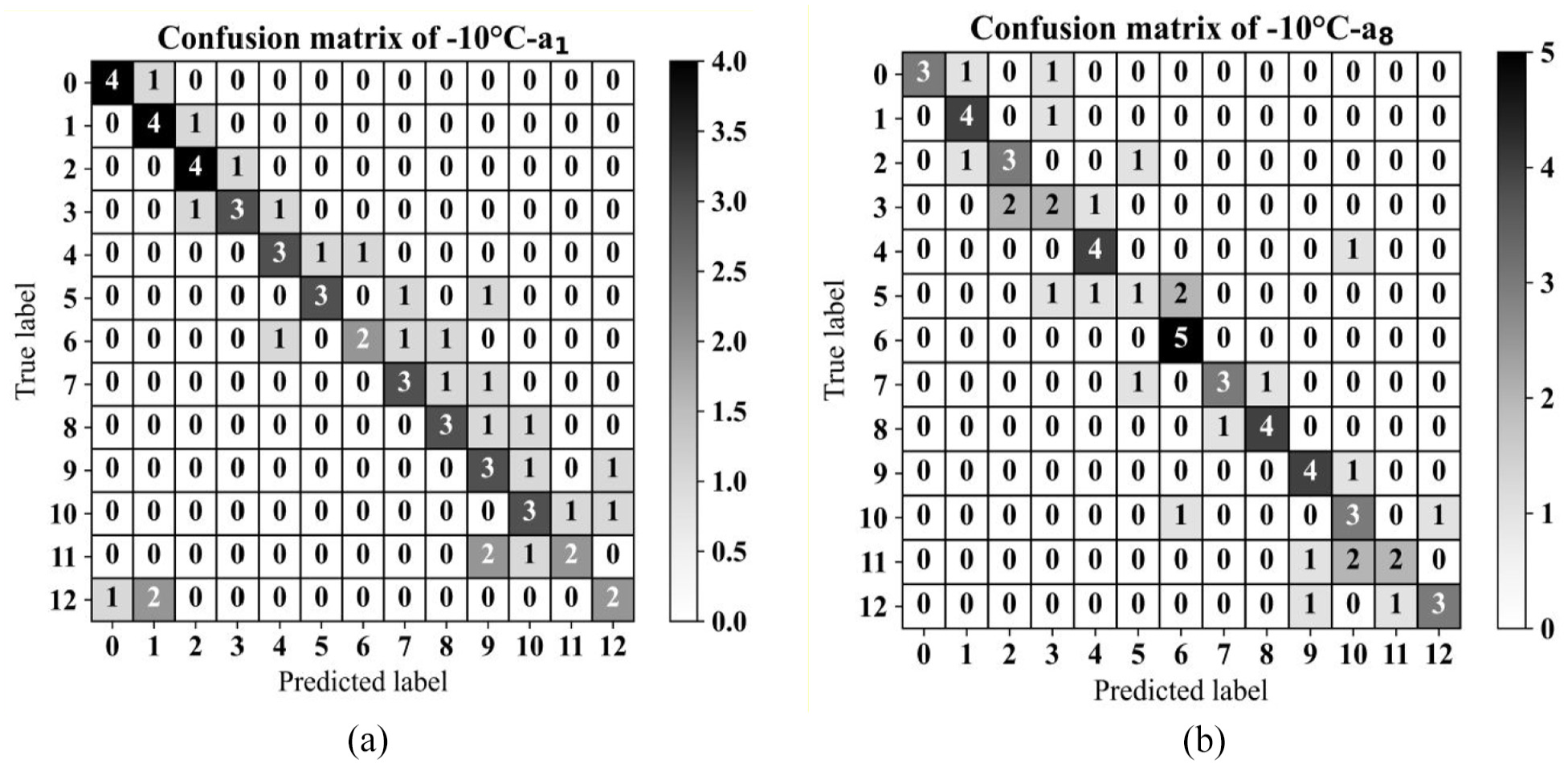
To compare the designed framework with the previously introduced TL models, a DANN 46 was implemented on the raw vibration signals, assuming data collected through sensors a1 and a8, and using data from −10°C as the target domain. The same source domain data were used for the training phase of the neural network. The DANN model was trained using the Adam optimiser with a learning rate of 0.001, a batch size of 64 and a gradient reversal layer weight of 1.0. Confusion matrices in Figure 15(a) and (b) reveal the outcomes of this domain adaptation.
Confusion matrices for the test phase utilising DANN for target domain data at −10°C and for (a) sensor a1 and(b) sensor a8.
The confusion matrices in Figure 15(a) and (b) illustrate that employing DANN achieved an accuracy of approximately 83% for sensor a1 and 85% for sensor a8. In comparison, the designed framework in this study, that is, UCTRF (confusion matrices in Figure 13(a) and 14(a)) resulted in a 15% improvement in classification performance for both sensor datasets.
Classification using TCA
A further comparison was conducted between the developed SHM framework and a feature projection technique, specifically, TCA, applied to the raw vibration signals following augmentation. In this comparison, the feature extraction stage was omitted, as TCA aims to project both source and target domain data into a shared feature space. An RBF kernel was selected for its non-linear mapping capabilities, and a grid search was performed to optimise the TCA hyperparameters, evaluating three values for each parameter, as shown in Table 6.
Hyperparameter grid search configuration for TCA implementation.
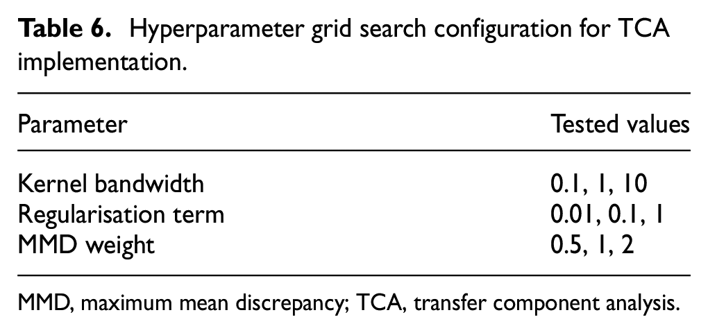
MMD, maximum mean discrepancy; TCA, transfer component analysis.
After training, validation and testing using data collected at +30°C for sensors a1 and a8 as the source domains (resulting in two separate networks) and data at 0°C for the corresponding sensors as the target domain, the optimised TCA model, with kernel bandwidth, regularisation term and MMD weight set to 1, 0.1 and 0.5 respectively, achieved accuracy values of 60% and 63% for the two scenarios (Figure 16(a) and (b)).
Confusion matrices for the test phase utilising TCA for target domain data at −10°C and for (a) sensor a1 and(b) sensor a8.
Figure 16 demonstrates that TCA is not able to project source and target domain data so properly even in its optimised structure. The subpar performance of TCA is attributed to its static feature projection approach, which lacks the adaptability to domain shifts and hierarchical feature learning inherent in the developed framework.
Weight adjustments in mitigating EOVs
As previously mentioned, instance-based domain adaptation methods aim to recalibrate the weights of the source and target domain observations to mitigate distribution discrepancy in these domains. In this approach, for the implementation of TrAdaBoost, all instances from the source and target domains initially received an equal weight (0.0022). As the adaptation progressed, the weights of source domain instances that closely resembled those in the target domain increased, while those less related to the target domain decreased. Conversely, in the target domain, weights for instances that could not be classified correctly in the adaptation process increased, whereas those correctly classified in the initial stages saw their weights decrease.
To illustrate this dynamic, weights allocated to the source domain data at 5°C and to the target domain at −15°C (both captured using sensor a1) were used as examples. To present the process of EOVs mitigation using the employed domain adaptation, selecting feature spaces where there are intersections between various classes’ observations as well as source and target domain data can promote better visualisation. To this end, feature numbers 26 and 84 which are lower ranked than the first and second features (as depicted in Figure 11) were selected. The weight changes for these two domains in the first, 500th and last epochs are depicted in Figure 17(a) to (c). The scaled version of weights was utilised for the size of the plotted scatters, in such a way that the initial weight (0.0022) was changed to 300 and the other weight values were altered based on this; the minimum weights, close to 0, were also scaled to 50.
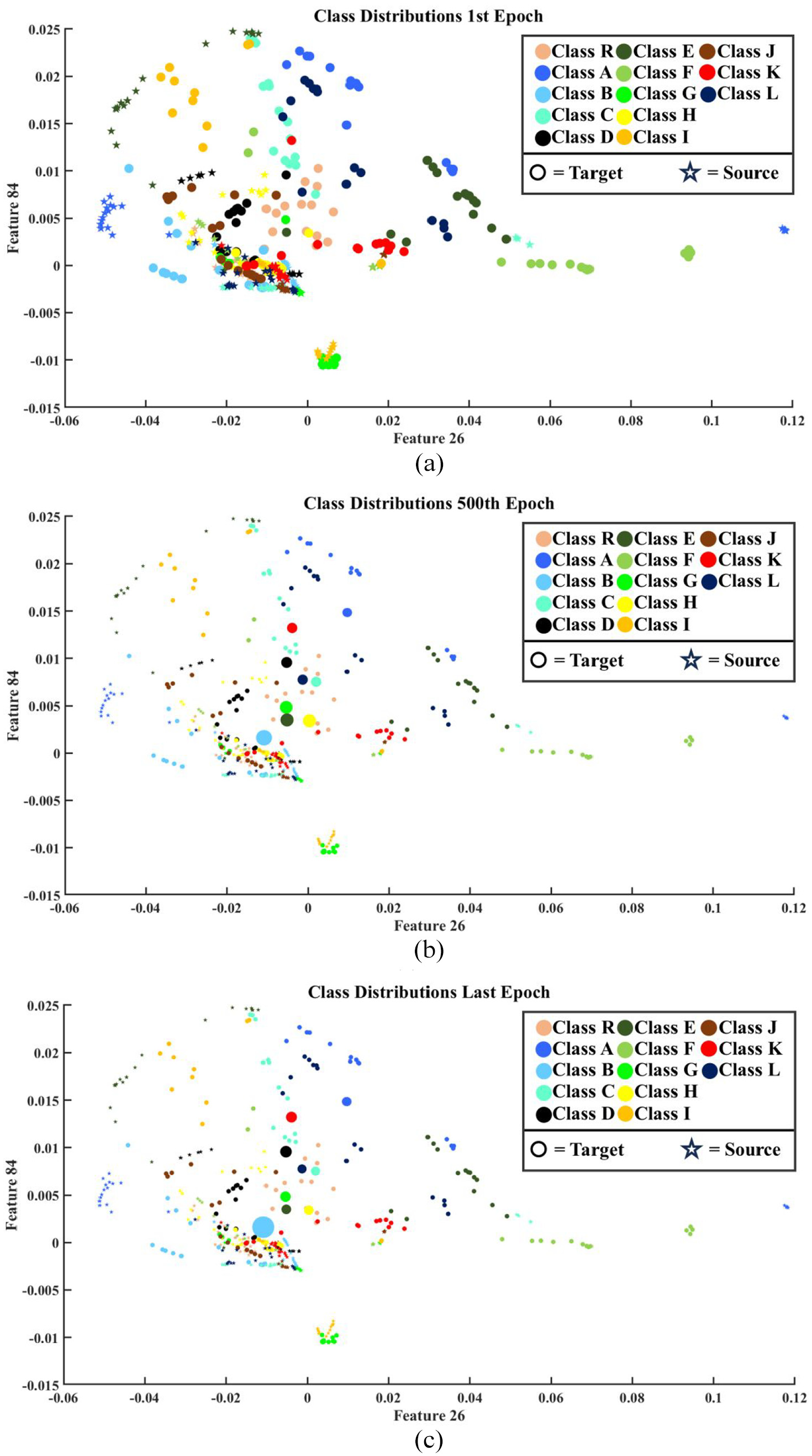
Scaled weight changes of the source and target domain instances at (a) the first epoch, (b) the 500th epoch and (c) the last epoch.
Evaluating the above scatter plots, it can be understood that the weights assigned to the source domain instances decreased dramatically, as the existing differences between the source and target domains’ distributions made the source domain observations unhelpful for classifying the target domain instances. For the target domain, on the other hand, the weights of the observations almost decreased because those samples were correctly classified upon initiating the domain adaptation framework (thanks to the capability of the applied hybrid feature extraction model). However, for several instances, the allocated weight increased because their classifications were challenging for the classification network. With greater precision, it can be understood from Figure 17 that these instances were mainly located near the clusters of other classes. For example, the weights of an instance from Class B, characterised by a light blue colour, increased significantly because it was positioned near a cluster of observations from Class I, which is marked by an orange colour, as well as a limited number of samples from Class D, distinguished by black.
The weight changes for a couple of observations are depicted in Figure 18 (in their original magnitude and before the scaling stage) for the target domain (−15°C) throughout the entire epoch numbers. Each of these instances belongs to one of the 13 classes; these instances were selected as they revealed more fluctuating behaviour among their counterparts in each class. It should be noted that the differences between the instance indices and class labels stem from the fact that the target domain data were divided into the train and test subsets in a shuffled manner.
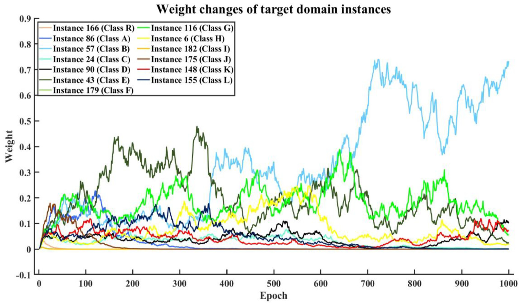
Class-wise weight changes of selected target domain instances at −15°C.
It is worth noting that for some of the fault scenarios, the weight changes of the selected instances are so slightly separate from the remaining damage conditions, but almost all the weight’s amplitudes reached under 0.1, and only for one case, that is, Class B the increasing trend of the allocated weight continued until the last epoch. Besides the closeness of instances to the clusters of other categories, an observation that will be an outlier will receive greater weight during the process of the domain adaption in an instance manner.
The applied TL technique iteratively adjusts the visualised weights for each temperature scenario until the desired epoch is reached, enhancing the accuracy of classifying divergent health conditions. Opting for a more precise feature extraction technique may help the TL approach achieve convergence more quickly. Moreover, choosing a feature extraction or data projection method that identifies a common space for the data distribution of both source and target domain observations can increase the weights in the source domain and expedite convergence.
Practical considerations and applicability
The proposed framework was implemented on a cluster with 72 CPU cores and 200 GB of RAM. DR using UMAP required 1.5 min per health scenario, CapsNet training took 45 min for 200 epochs and domain adaptation using TrAdaBoost was completed within 5 min per boosting iteration.
The modular nature of the framework allows it to be deployed on cloud platforms, such as Azure. For instance, the computational tasks can be parallelised and distributed across virtual machines or containers using tools such as Azure Batch. Furthermore, the framework’s reliance on vibration signal data ensures straightforward integration with pre-existing monitoring pipelines, without requiring specialised data formats. The lightweight architecture of CapsNet and TrAdaBoost ensures that the framework is both scalable and adaptable to different WTB configurations and evolving environmental conditions.
Conclusion and future work
This paper proposed an SHM framework, UCTRF, tailored for the classification of structural conditions in WTBs amidst variable environmental conditions, notwithstanding the limitation of training data. UMAP was integrated for feature extraction with CapsNets, supplemented by TrAdaBoost and a Random Forest classifier, to create a robust method capable of correctly classifying over 95% of health scenarios. The success was found in the synergistic use of UMAP for preserving data structure in reduced dimensions, CapsNets for interpreting spatial relationships and TrAdaBoost for transferring knowledge from analogous tasks, making the framework highly effective for accurate damage diagnostics in varied environments, with the potential for real-time application.
The most notable finding was that the TL-based methodology enabled robust damage classification in WTBs across a wide temperature range (–5°C to 35°C), even with limited training data (20 observations), making it viable in various industrial settings. Similar results were obtained regardless of sensor selection (a1 and a8), demonstrating the algorithm’s effectiveness across different locations on the WTB, that is, highlighting the model’s adaptability and reliability for empirical defect diagnosis under uncertain environmental conditions.
While the method successfully addressed uncertainties related to temperature variations, its evaluation was restricted to a single WTB model and experimental setup. This limitation arose due to the inherent challenges of accessing broader datasets or replicating comparable experimental conditions for other WTB configurations. Future work should explore extending the framework to datasets generated via finite element modelling or less complex structures, such as composite plate-like materials, as performing tests simulating EOVs is more practical with appropriate chamber setups. Additionally, while this study focused on surface-level damages, primarily linked to vibrational signals that remain largely unaffected by humidity or wind speed variations, future investigations should incorporate these variables alongside other factors, such as material degradation and structural modifications, to further enhance the framework’s generalisability. Incorporating diverse excitation modes and sensor configurations would also provide a more comprehensive evaluation of its robustness under real-world conditions.
The integration of advanced ML techniques or DL architectures could further improve the classification accuracy and computational efficiency of the model. Real-time implementation and validation of the framework on operational WTBs would be a significant step towards practical deployment, enabling continuous monitoring and early detection of potential damages.
In conclusion, the UCTRF framework demonstrated significant potential for accurate and reliable damage classification in WTBs under variable environmental conditions, even with limited training data. By addressing additional sources of uncertainty and expanding the scope of study, future research could advance SHM for WTBs further contributing to the efficiency and safety of wind energy generation. Continued development in this field holds promise for more resilient renewable energy infrastructures and optimised maintenance strategies.
Footnotes
Declaration of conflicting interests
The author(s) declared no potential conflicts of interest with respect to the research, authorship and/or publication of this article.
Funding
The author(s) received no financial support for the research, authorship and/or publication of this article.