
Abstract
Reinforced concrete (RC) structures are well-known for their high durability; however, they remain vulnerable to natural hazards and extreme events that can impact their performance over time. In aggressive environments, there is a high likelihood of increased maintenance, rehabilitation, and repair actions that constitute a significant portion of the total lifecycle spending. Monitoring systems have been implemented during the last decades to collect periodically or continuously essential data about the durability performance of the structures in real operation. However, the effectiveness of these systems is impacted by sensor efficacy, influenced in turn by environmental factors, sensor durability, and power outages, leading to intermittent or permanent data gaps. This study proposes a methodology to address the problem of missing data of a Structural Health Monitoring (SHM) system, specifically aiming to provide more accurate and continuous information from concrete resistivity and temperature sensors to support the early detection of corrosion. The proposed methodology was applied to a repaired RC structure with over fourteen years of data, where significant gaps in the measurements were present. The approach combines several techniques to fill these gaps: deep machine learning for air temperature, generalized linear models for concrete temperature, and pattern recognition for concrete resistivity. To the best of the authors’ knowledge, this is the first time a methodology has been proposed for imputing missing data from resistivity sensors in SHM systems, which are increasingly being implemented. This approach is innovative and offers potential benefits for SHM system managers, providing more information on long-term sensor data that could aid in early corrosion detection and maintenance planning. The application of the proposed methodology to a real case study indicated a successful imputation of 43.4% of missing data although some challenges persist for sensors located in areas characterized by high measurements variability.
Keywords
Introduction
Reinforced concrete (RC) structures bridges play a crucial role in modern infrastructure, providing vital connections between communities and facilitating the continuous flow of people and goods. The long-term lifespan of these structures is essential to ensure the ongoing functionality of the transportation network. Therefore, the maintenance of these bridges relies on their ability to withstand operational and environmental challenges, thus providing reliable and safe service. Climate conditions and extreme events can affect the goal of maintaining and extending the lifespan of RC bridges. 1
Chloride ingress produced by climate conditions is the main corrosion mechanisms impacting durability of RC structures in coastal areas, where the exposure to saltwater accelerates the corrosion process. 2 Under natural exposure conditions, the rate of corrosion in reinforcing steel varies significantly due to several uncertainties including concrete properties. 3 Therefore, corrosion evolution is a complex phenomenon that initiates internally within the structure and can affect long-term structural safety and reliability without timely detection through inspections. 1 Hence, there has been a growing interest recently in the use of Structural Health Monitoring (SHM) systems in reinforcement concrete structures to gather information about current state of the materials and to detect early corrosion.4,5 This is because sensors could provide real-time information about the condition of the structure, which can be crucial for making informed decisions about maintenance schedules and repairing techniques.
One of the challenges associated with long-term SHM is ensuring continuous measurements during the service life of the structure. However, some periods could not be monitored due to several factors, such as power outages, sensor malfunctions, data transmission issues. In addition, certain data points also might be missing due to signal noise. Thus, missing data can occur in any experiment, and researchers typically address this issue by either recovering the information or imputing the missing data. 6 The effectiveness of data imputation methods is significantly influenced by the quality and quantity of the available data. 7 Various statistical imputation methods allow for the estimation of missing data, including mean imputation, spatial or temporal correlation, other statistical techniques, and machine learning algorithms.8–10
Addressing the problem of missing data has been a subject of investigation in various research domains and has recently gained traction in the field of SHM.8,11,12 Liu et al. 13 worked with accelerometers and presented a multivariate time-series analysis method for infrastructure damage detection, using a state-space embedding approach and singular value decomposition. The proposed approach demonstrates computational efficiency and successful damage identification in validation tests on a linear spring–mass system and a benchmark experimental structure. Wan and Ni 14 presented a methodology for SHM data recovery on temperature and accelerometers sensors using Bayesian multitask learning with a multidimensional Gaussian process prior, efficiently modeling multiple tasks and their interrelations. The proposed approach demonstrates superior performance in reconstructing SHM data compared to traditional Bayesian single-task learning, with a focus on the impact of covariance function selection. Li et al. 8 address the issue of missing time series data in SHM systems, focusing on the calculation of cable force by constructing a matrix of correlations between days and within one day, and employing a probabilistic principal component analysis (PPCA) method to improve data imputation. The results show that fully capturing temporal correlations from measured values enhances imputation accuracy, with PPCA outperforming PCA, particularly in scenarios with continuous missing data, highlighting the potential for improved imputation by considering temporal correlations across dimensions. Niu et al. 15 also focused on cable force data and proposed a spatiotemporal graph attention network for restoring missing data in SHM systems, focusing on the spatial and temporal dependencies within the sensor network. Jiang et al. 16 proposed a novel data-driven generative adversarial network to impute missing strain response data from wireless sensors in SHM systems. The method was verified on a real concrete bridge and demonstrated superior imputation accuracy and efficiency by leveraging spatial–temporal relationships among strain sensors without needing a complete dataset during training. More recently, Gao et al. 11 presented a slim generative adversarial imputation network (SGAIN) for recovering missing deflection data of SHM systems in a highway–railway dual-purpose bridge. The model used slim neural networks with a generator–discriminator architecture to efficiently impute missing data caused by sensor malfunctions or communication outages. The SGAIN network presented superior performance and execution speed when compared to the conventional GAIN model.
Other types of sensors have been also analyzed. Tang et al. 17 developed a convolutional neural network for recovering multichannel SHM data with group sparsity awareness, effectively addressing segments of continuous missing data. The method demonstrated strong recovery performance on synthetic, field-test, and seismic response monitoring data. More recently, Luo et al. 18 analyzed the quantification and prediction of pitting corrosion of steel structures in using one-dimensional convolutional neural networks (1D CNN) in conjunction with electromechanical impedance (EMI) sensors. By using an EMI-instrumented circular piezoelectric–metal transducer, it was possible to detect corrosion-induced mass loss. The results showed high accuracy in predicting the extent of pitting corrosion, laying a technical foundation for real-time and quantitative monitoring of corrosion in steel structures.
The studies mentioned above have significantly contributed to deal with missing data estimation in SHM systems for different type of sensors (see Table 1). However, to the best of the author’s knowledge, no research has been published regarding the imputation or filling of missing data for SHM durability sensors, in particularly, concrete resistivity sensors on reinforcement concrete structures.
Publications on data imputation methods used in SHM systems.
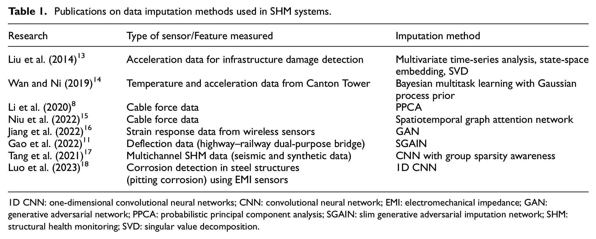
1D CNN: one-dimensional convolutional neural networks; CNN: convolutional neural network; EMI: electromechanical impedance; GAN: generative adversarial network; PPCA: probabilistic principal component analysis; SGAIN: slim generative adversarial imputation network; SHM: structural health monitoring; SVD: singular value decomposition.
Concrete resistivity sensors have proved to be useful for collecting information on chloride contamination and to be durable for long-term monitoring, which is particularly important, resulting in regular installations of sensors for SHM systems. 19 However, several external factors may affect the electrical resistivity of concrete.20,21 Given the significant influence of temperature on resistivity, the installation of concrete temperature sensors is common when considering concrete electrical resistivity sensors, to account for temperature variations in data analysis. 20
In this study, we introduce a novel approach that focuses specifically on filling missing data for SHM durability sensors, particularly concrete resistivity sensors, which has not been addressed in previous research. The novelty of this research lies in the development of a comprehensive methodology that integrates multiple techniques for imputing missing sensor data, enhancing the reliability of long-term corrosion monitoring and is tested on a SHM system in a RC bridge for over ten years period. The article presents a methodology to fill missing data found within the use of resistivity and temperature sensors on SHM system. The proposed methodology uses an external input, which is air temperature, to improve the estimation of missing data. However, the external input also had missing values that needed to be adjusted. To address this, first deep learning, specifically a feed-forward neural network, was implemented. Due to the high correlation between air and concrete temperature, generalized linear models were applied to estimate the missing concrete temperature values. Finally, the missing data for the resistivity sensor was estimated using pattern recognition and the inverse relationship between temperature and electrical resistivity. The results suggest that the proposed methodology can serve as a valuable tool to enhance the quality of sensor data and improve the effectiveness of monitoring systems in the analysis for early detection of corrosion. The article is structured as follows: section “Case study description” describes the case study, section “Proposed methodology” presents the methodology employed, section “Results and discussion” provides the results and discussion, and finally, the research conclusions are presented in section “Conclusions”. The code created for this research is available at https://github.com/LuisRinconP/Missing-Data-Estimation-Method-for-Durability-Survey-of-Reinforced-Concrete-Structures.
Case study description
Test bed description
The bridge, inaugurated in the 1980s, is located in central Portugal. It features a main span of over 200 m and a total length of more than 900 m, supported by 85 m high piles in the tallest section. The analyzed bridge is located less than 5 km from the sea and serves to connect two regions of one of Portugal’s major cities.
A detailed inspection revealed several issues: low execution quality with concreting defects, poor-quality painting of steel structures, reinforcement corrosion, alkali–silica reactions, sulphate attack (primarily in the foundations of the bridge), and frequent cracking in prestressed girders. These factors, along with updated design codes, dictated a rehabilitation of the structure in the 2000s. Additional information about the structure cannot be disclosed due to confidentiality concerns.
Concrete electrical resistivity and temperature data were collected from five repair zones on the bridge. The objective of the SHM system is to obtain information about the progress of the despassivation front in the concrete. Data collection occurred daily from July 2006 to November 2020.
Sensors and measurements
The air temperature data were obtained from the Instituto Português do Mar e da Atmosfera (IPMA), a public institute under the indirect administration of the state. The data come from an automated weather station located less than 5 km from the analyzed bridge. The station is situated 4 m above sea level, and the daily average temperature, measured at a height of 1.5 m, was used.
Sensors were installed in five repaired zones of the structure, referred to as Location 1 (L1) through Location 5 (L5). Concrete electrical resistivity was measured using a two-graphite electrode resistivity sensor. Installation involved removing the concrete cover, placing the electrodes at depths of 15 mm and 30 mm, and then replacing the cover. Eight resistivity sensors were installed and will be referred to as L1–R1 if the sensor is located in Location 1 at a depth of 15 mm, and L1–R2 if it is in Location 1 at a depth of 30 mm. The concrete temperature was measured using a PT100 thermometer embedded in concrete installed at the same time. The temperature sensors will be named L1-T if located in Location 1, and similarly for the other locations. Data acquisition was performed automatically daily at midnight using a Datataker 500. The two-graphite electrode resistivity sensors measure daily concrete electrical resistivity of the bridge (Figure 1(a)). The concrete temperature was measured in Celsius using the same daily frequency (Figure 1(b)). After more than fourteen years of measurements, several data are loss due to problems with the data acquisition system and the power supply unit of the data acquisition system. A total of 27,032 electrical resistivity data points and 19,205 concrete temperature data points were collected, from eight resistivity sensors and five temperature sensors. Figure 2 presents the missing data for each of the sensors considered in this study, highlighting significant gaps in the concrete resistivity sensors.
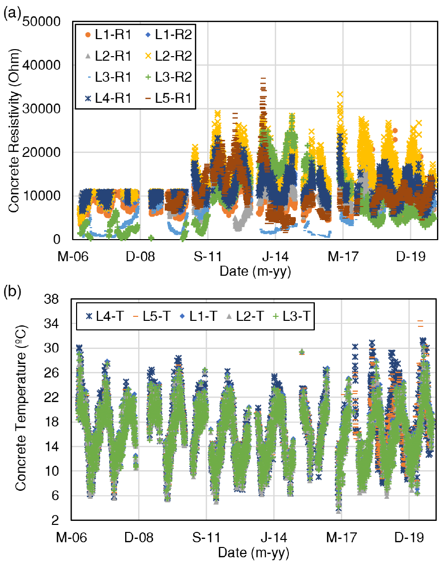
(a) Concrete electric resistivity and (b) concrete temperature data obtained between 2006 and 2020.
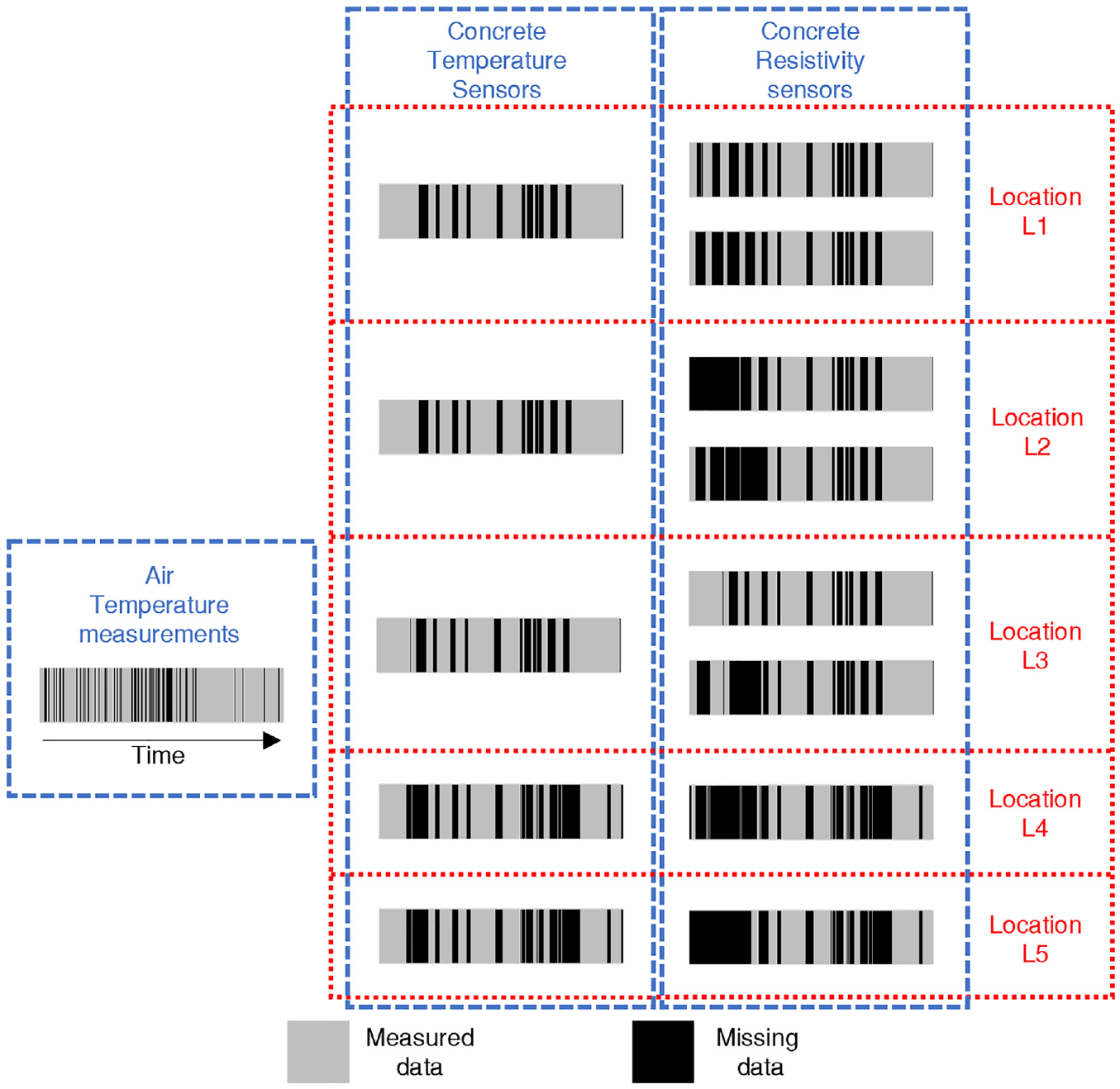
Missing data of each sensor consider in this research.
Proposed methodology
The methodology proposed for addressing missing data in this SHM system encompasses four key stages. This approach begins with assessing the sizes of data gaps (stage A), followed by procedures to fill gaps in air and concrete temperature data (stages B and C), and concludes with the implementation of pattern recognition techniques for missing resistivity data (stage D). Each phase aims to systematically tackle the absence of information in the sensor datasets, ensuring a comprehensive approach to data completion. Figure 3 presents a diagram of the methodology used in this article to fill in missing data from the concrete resistivity and temperature sensors, where the key stages are highlighted. Stage A presents a recommendation for data imputation based on the size of the data gap. Stage B introduces the methodology using artificial neural networks to fill the missing data from the air temperature sensor (explained in section “Feed-forward neural network method”). Stages C and D detail the methods for imputing missing data from concrete temperature and electrical resistivity sensors, which are described in sections “Generalized linear models” and “Group pattern recognition,” respectively.
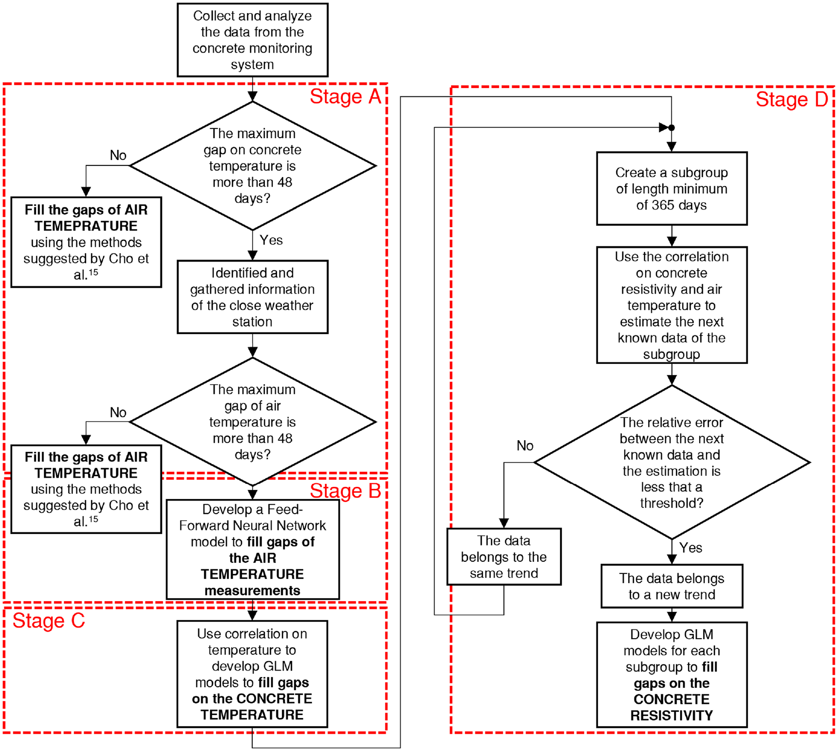
Flowchart of the methodology proposed to fill the missing data of the concrete resistivity sensors.
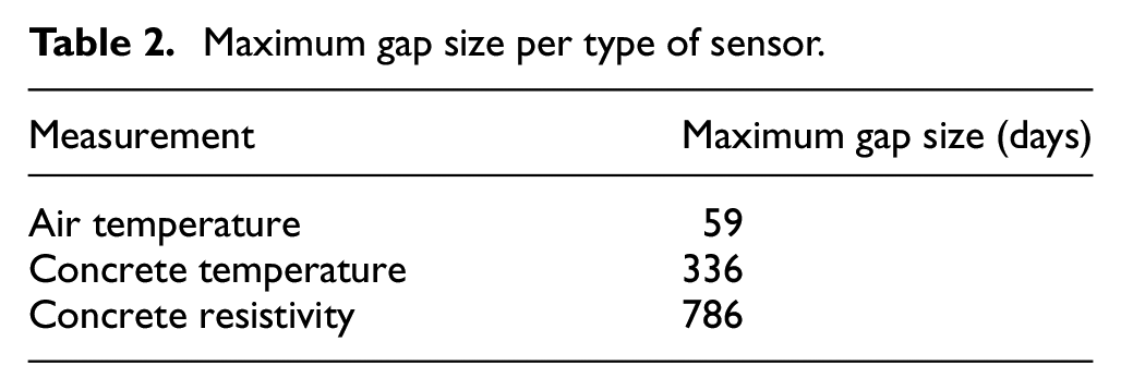
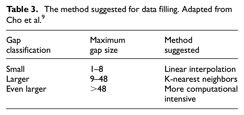
The methodology starts with the first part of stage A (see Figure 3), which consists in analyzing the maximum size of the gap to be filled. Table 2 presents the maximum sizes obtained for missing gaps. It is observed that the concrete temperature and resistivity present gaps of more than 1 year of lost information. Cho et al. 9 presented an extensive study to establish the best data imputation methods. In their study, three levels of gaps are established and numerical methods for filling are suggested (Table 3). The methodology proposed in this article suggest following these recommendations. Therefore, for the missing concrete temperature and resistivity data require more intensive computational methods.
Maximum gap size per type of sensor.
The method suggested for data filling. Adapted from Cho et al. 9
Lo Presti et al. 6 presented a methodology for estimating missing data, primarily applied to rainfall data in Italy. The methodology is divided into two stages. First, they identify a similar weather station to the one being analyzed to determine suitable similarity coefficients. Second, a regression method is applied to estimate the missing data. A similar methodology is employed for filling the concrete temperature data gaps. Therefore, air temperature data are collected from a weather station located 3.1 km away from the analyzed structure. However, this station also has missing data, with a maximum gap size of 59 days, which is smaller than those in the structure sensors but still significant according to Cho et al. 9 . In this initial step, a deep machine learning technique, specifically a feed-forward neural network, is used to compute the missing values of air temperature (stages A and B, see section “Feed-forward neural network met”). Then, the proposed methodology considers the high correlation between air temperature and concrete temperature, to impute the missing data in the concrete temperature sensors (stage C, see section “Generalized linear models”).
Temperature is a crucial factor in the resistivity of concrete. However, it is important to recognize that it is not the only factor. According to the literature, concrete resistivity is affected by several factors such as pore structure, ion composition in pore water, cement content, and the degree of saturation, among others. 22 Temperature impacts resistivity by altering ion mobility, ion–ion and ion–solid interactions, and ion concentration in the pore solution.22,23 Typically, as the temperature of concrete increases, its electrical resistivity decreases. 24
The relationship between electrical resistivity and electrical conductivity is commonly expressed as an inverse linear correlation.24,25 Although temperature is not the sole influencing factor, it was chosen for this study due to its significant impact and the availability of temperature data from the sensors. Since comprehensive information on all factors influencing resistivity was not available, methods were employed to learn from the temperature–resistivity relationship in real conditions and attempt to extrapolate this relationship (stage D, see section “Group pattern recognition”). Although this represents a limitation of the study, it is decided to fill the resistivity gaps using an intensive computational method that associates these parameters, considering the missing data on temperature and resistivity as missing at random. 26
Feed-Forward Neural Network method
As mentioned in the previous section, when there are gaps of more than 48 consecutive data points, more intensive computational methods must be used for data imputation. This section presents the Artificial Neural Networks method used to fill the missing data for the air temperature sensor, corresponding to stage B in Figure 3.
Artificial neural network models comprise a collection of neurons processing information individually and simultaneously, mirroring the functioning of the human brain,
27
significantly enhancing the predictive accuracy by effectively capturing complex patterns in the data. In the context of time series forecasting, the multilayer feed-forward neural network autoregressive (FFNN-AR) model,
28
stands out since it considers the evolution of time series data by integrating an autoregressive process of order
In this context, the temperature–lagged time series estimates are the inputs

The number of neurons
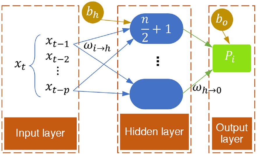
Structure of the FFNN-AR model. Adapted from Rincon et al. 27
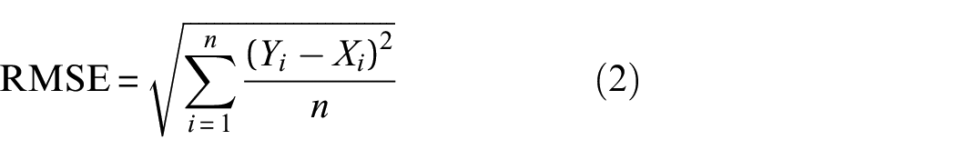
The choice of the activation function in the layers corresponds to the type of the problem being solved and the nature of the input and output of the layers, and is determined through the loss function, that is, root mean square error (RMSE) indicator (Equation (2)) which provides a measure of accuracy by measuring the average magnitude of the differences between the predicted (Y) and the actual values to minimize the difference. In this study, the activation function for the hidden layer is a non-linear sigmoid activation function (Equation (3)). A linear activation function (Equation (4)) is applied for the output layer since the predictions in the output layer are the weighted sum of the resulting weights and biases from the hidden layer, making it directly proportional relation:
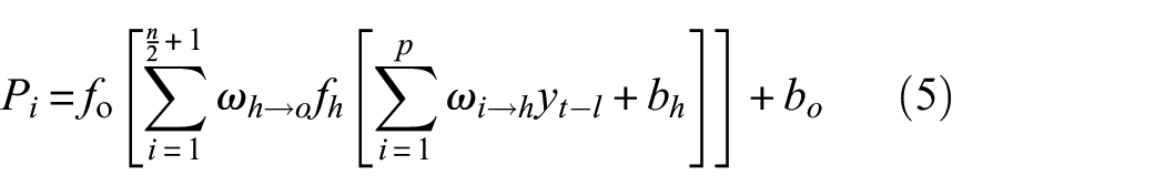
The FFNN-AR model (Equation (5)) considers the dynamic behavior of time series by implementing nonlinearity within the hidden layer to represent nonlinearly the autoregressive process through a nonlinear activation function (Equation (3)) to the weighted sum of the inputs
The FFNN-AR model was trained on temperature measurements for the interval from July 04, 2006 to September 16, 2006 and validated by predicting the temperature measurements from September 17, 2006 to October 04, 2006. The architecture of the FFNN-AR model consists of 15 nodes in the input layer, a hidden layer with eight nodes using a sigmoid activation function, and a single-output node. Training was conducted over 100 epochs using the Adam optimizer with a learning rate of 0.001. The loss function used for training was the RMSE, with a final training RMSE of 0.0003°C.
Figure 5 presents the comparison between the predicted and actual temperature measurements from September 17, 2006 to October 04, 2006, demonstrating good agreement between the two. Table 4 provides the validation error metrics: mean error (ME), mean absolute error (MAE), and RMSE, with values of −0.098°C, 0.99%, and 1.34°C, respectively. The model’s performance was stable, as indicated by the low RMSE and MAE values.
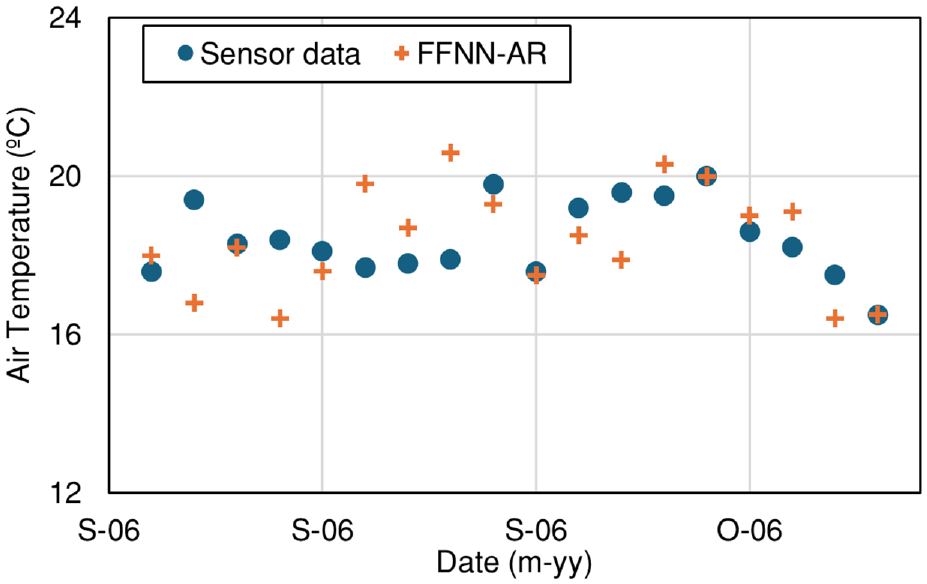
FFNN-AR model validation.
Validation error indicators.
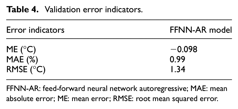
FFNN-AR: feed-forward neural network autoregressive; MAE: mean absolute error; ME: mean error; RMSE: root mean squared error.
Generalized linear models
Another intensive computational method used in the proposed methodology is Generalized Linear Models (GLMs). These are employed when a variable significantly influences the results of another variable. In this case, this model is part of stages C and D in Figure 3, where the predictor variable, air temperature, is used to estimate the values of concrete temperature and concrete electrical resistivity.
Generalized Linear Models (GLMs) constitute a statistical framework that extends classical linear regression models. These models have found widespread use in civil engineering due to their ability to provide greater flexibility in data distribution and the relationship between the dependent variable and the independent variables.29–31
In a GLM, the relationship between the response variable
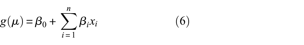
where
Gaussian family distribution was applied for the error function due to the suitable for this problem according to the main key metrics used, including pseudo
Group pattern recognition
To achieve better results with the GLMs, a group pattern recognition algorithm was implemented to identify variations in the readings of the concrete resistivity sensors. These variations could be due to degradation processes or changes in other factors influencing the sensors that were not considered in this study. This step corresponds to Stage D in Figure 3.
Pattern recognition for subgroup creation focuses on identifying and understanding patterns and structures within datasets involving multiple distinct groups or classes. The group-based approach aims to identify similarities and differences among datasets that can be divided into distinct groups or categories, aiding in better prediction of missing data. Various techniques exist to address group pattern recognition. The two primary methods focus on clustering algorithms and classification techniques to assign data to different classes or groups based on their characteristics. 32 Clustering algorithms were used in the group pattern recognition for thisarticle. Correlation was used as the variable to separate different subgroups.
Results and discussion
This section presents the results of the proposed methodology for the case study described in section “Case study description.” In section “Filling missing air temperature data”, the missing data in the air temperature measurements are estimated, while in section “Filling missing concrete temperature data” the results obtained in filling the missing data for the concrete temperature sensors are presented. Section “Filling concrete resistivity data” outlines the final part of the methodology, focusing on filling the missing data for the resistivity sensors.
Filling missing air temperature data
The first step in Figure 3 is to compute the missing air temperature data. This was achieved using a feed-forward neural network (FFNN), as explained in section “Feed-forward neural network method.” The recorded air temperature data were used to train and validate the model. Table 5 presents the amount of known and missing data, and the largest continuous gap of missing data of the air temperature sensor.
Information about the missing data in air temperature database.
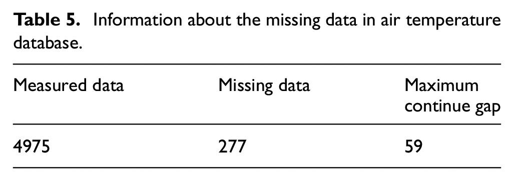
Figure 6 presents the results of the FFNN method for filling missing air temperature data. It is observed that the calculated values align adequate with the temperature variations produced by the sensors. To estimate the approximation accuracy of the FFNN, five artificial gaps of 1, 5, 10, 25, and 60 days were created. Table 6 presents the main error metrics obtained between all the artificial gaps and the values measured by the meteorological station. The MAE of 3.51 indicates that, on average, the values are off by 3.51°C, which is an acceptable value for the study. The
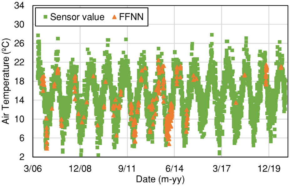
Data filling of air temperature using the FFNN method.
Principal error indicators for the FFNN method.
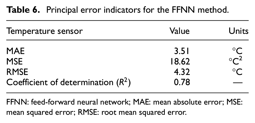
FFNN: feed-forward neural network; MAE: mean absolute error; MSE: mean squared error; RMSE: root mean squared error.
Filling missing concrete temperature data
Once a gap-free air temperature database is obtained, the methodology is applied to the concrete temperature sensors. Table 7 displays the Pearson’s correlation coefficients between air temperature and the five concrete temperature sensors installed within the structure. Schober et al. 34 suggest that a Pearson’s coefficient between 0.7 and 0.89 can be considered a strong correlation. Therefore, with correlation coefficients greater than 0.8, the methodology used GLM to estimate missing data from the concrete temperature sensors. Table 7 also presents the amount of known and missing data, and the largest continuous gap of missing data of the five concrete temperature sensors. Two sensors (L4-T and L5-T) acquired less data and presented maximum continuum gap of 336 days.
Information about the missing data in concrete temperature sensors.
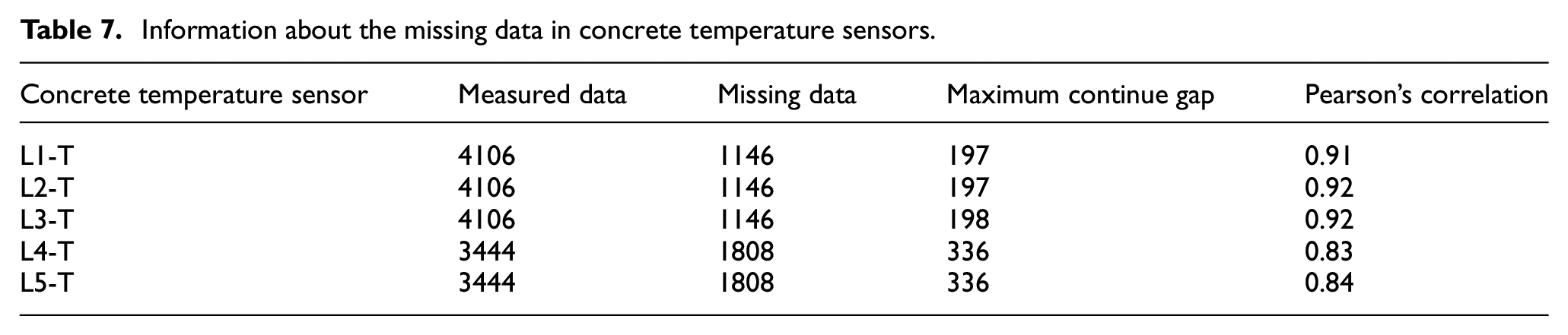
Figure 7 illustrates the results of filling missing data for the concrete temperature sensors. It is noteworthy that the estimations from the GLM adequately fill the gaps in the data for the five concrete temperature sensors. Additionally, a discernible seasonal trend is observed throughout the analyzed period that is also well represented by the filled data. Table 8 presents the primary error indicators for the series of the GLM model adjusted for each sensor. The L2-T and L5-T sensors show the best MAE and RMSE values, indicating greater precision when filling concrete temperature. However, the average MAE is 1.296°C, with low variability (standard deviation of 0.061), indicates that most sensors have similar precision in terms of mean absolute error. The average
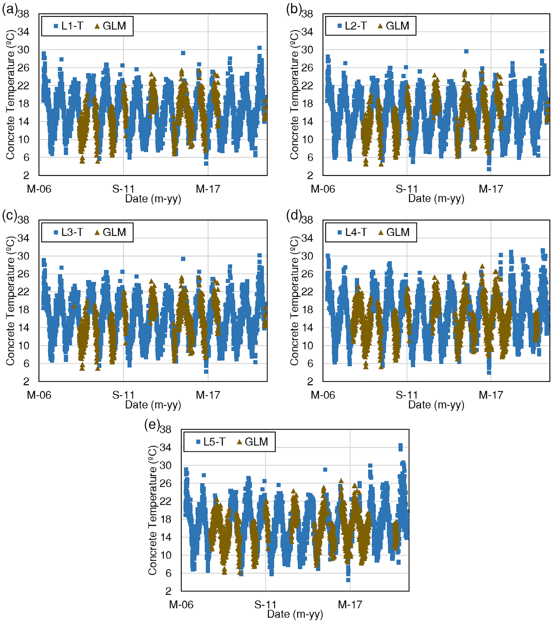
Data filling of the concrete temperature sensors using GLM for each sensor.
Error indicators for the GLM model.
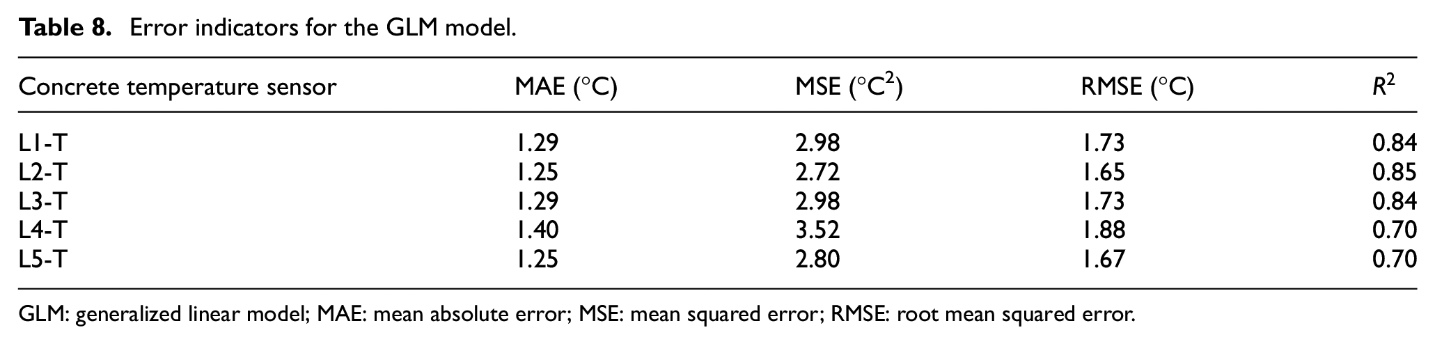
GLM: generalized linear model; MAE: mean absolute error; MSE: mean squared error; RMSE: root mean squared error.
Filling concrete resistivity data
The final step of the methodology is based on the premise of a correlation between temperature and electrical resistivity. This relationship is evident in Figure 8(a) and Table 9 where a negative correlation is observed for almost all cases. However, some sensors do not exhibit a clear correlation (Figure 8(b)). GLMs are consider on the estimation of the missing data in this section. However, the direct application of GLM is not feasible without first identifying patterns in the data. Therefore, pattern recognition techniques are employed to identify subgroups within the dataset that exhibit consistent trends, which then allows for the application of GLM for predictive purposes.
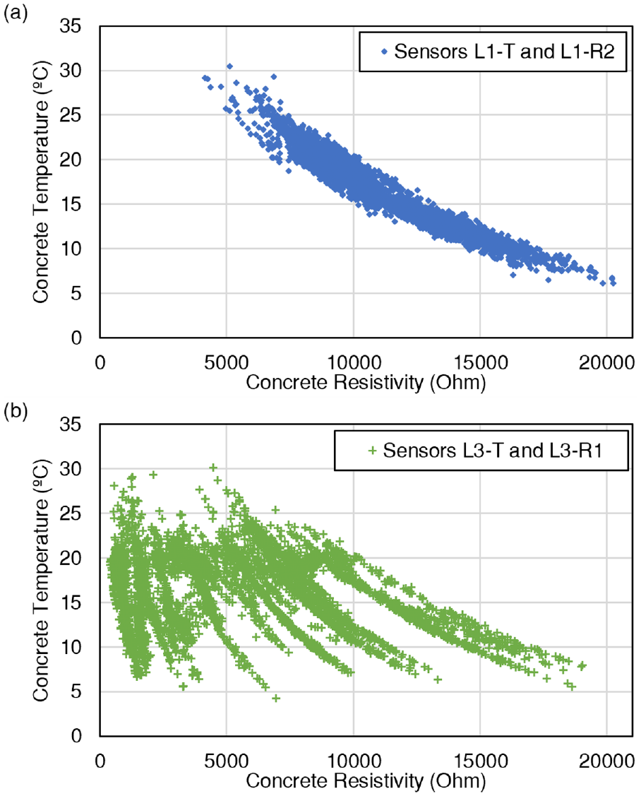
Relation between concrete temperature and resistivity sensors for sensor in location (a) L1 and (b) L3.
Pearson’s correlation between concrete resistivity and concrete temperature.
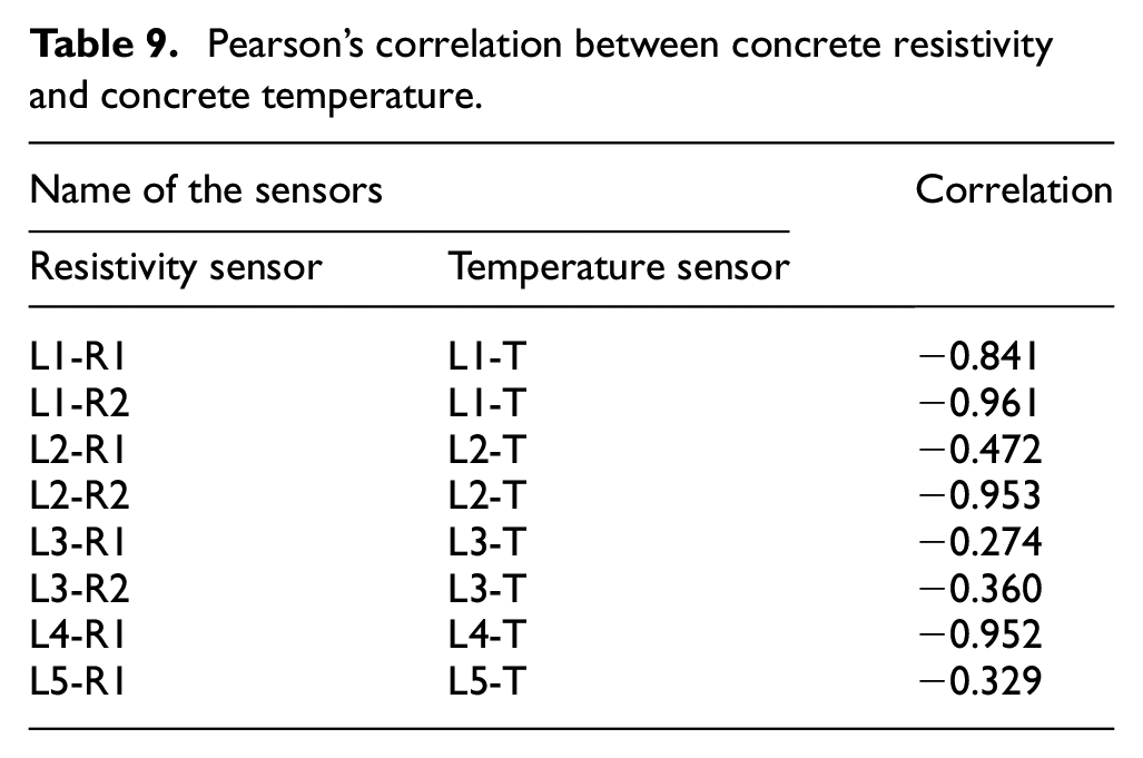
Figure 9 presents a 3D representation of Figure 8(b), highlighting the potential changes in correlation over time. These variations may be associated with fluctuations in concrete conditions. While the correlation varies, its association with temperature appears consistent. Hence, it is proposed to employ a group pattern recognition for resistivity data (stage D in Figure 3, see section “Group pattern recognition”).
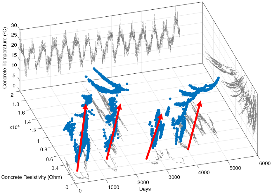
Relation of concrete resistivity, concrete temperature, and days of the sensors in location 3 (L3-T and L3-R1). In red, are possible different trends.
Group pattern recognition is used to identify subgroups among the analyzed sensors where data exhibit a consistent trend. The minimum subgroup size of 365 days was selected to reflect the seasonal cycles that influence concrete resistivity. This period was chosen because it aligns with typical climatic patterns, ensuring that the subgroups capture the variations that occur due to temperature and environmental changes over a complete year.
Starting from this minimum group size, a correlation is calculated, and the most recent data point is compared to the prediction using GLM. To minimize user-induced bias, the segmentation process was designed to be as objective as possible. We implemented a method that compares the relative error between the measured point and the prediction, triggering a new subgroup when this error exceeds a predefined threshold. This automatic procedure reduces manual intervention in subgroup creation, ensuring that the segmentation is based on statistical consistency rather than subjective visual interpretation. A relative error threshold of 0.8 was assumed based on engineering judgment to ensure good separation of subgroups during the pattern recognition process. When the error between the next measured point and the calculated prediction surpasses the threshold, a new subgroup is initiated.
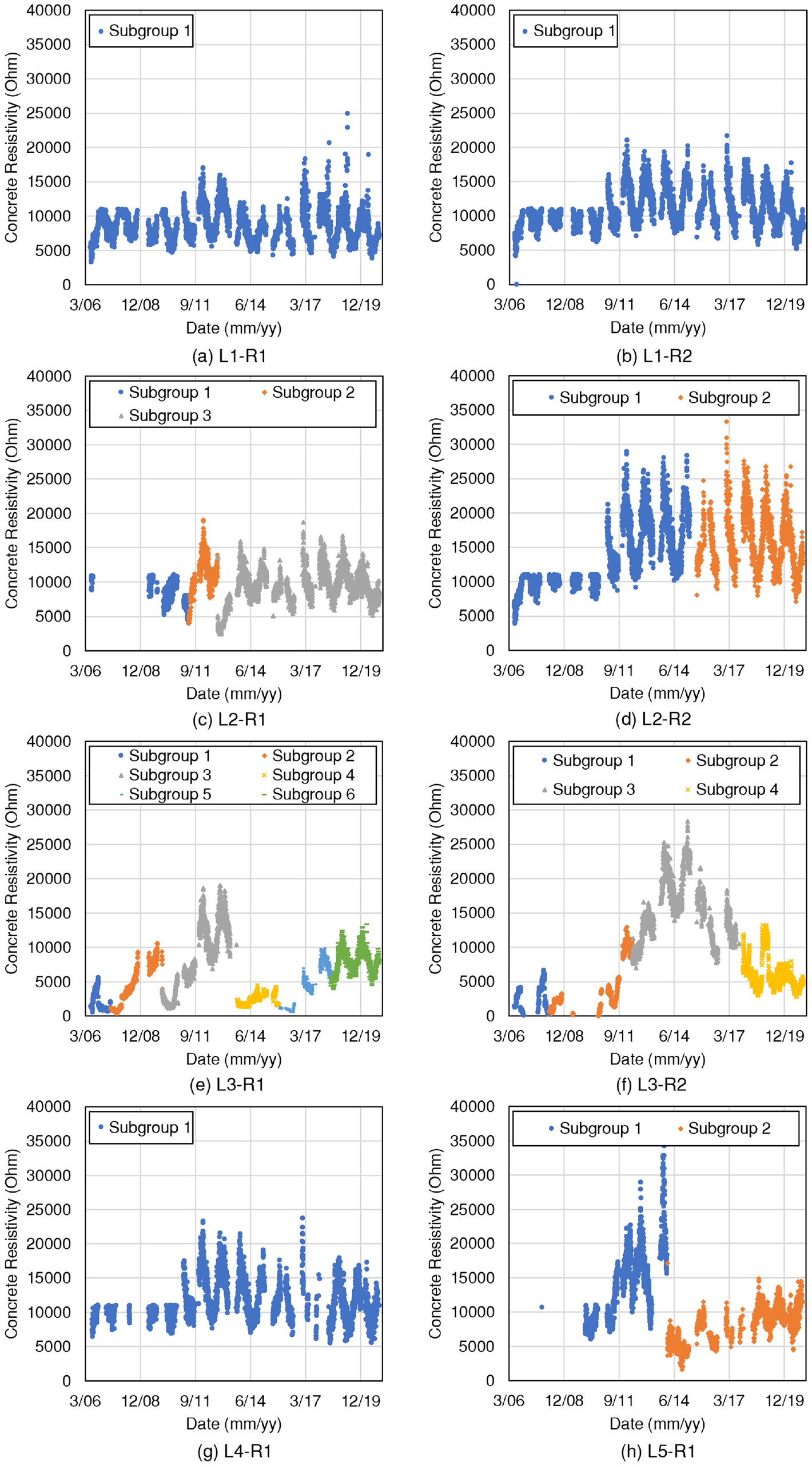
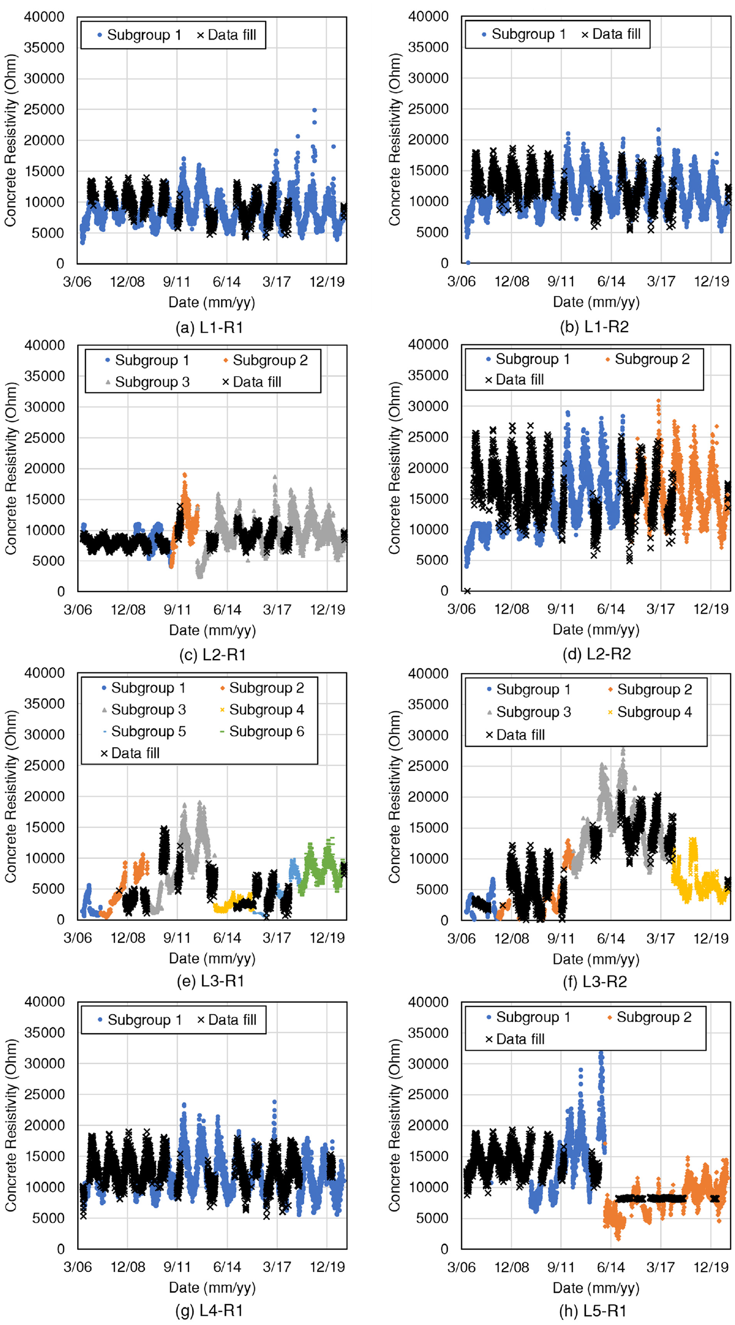
Figure 10 displays resistivity values segmented by subgroups, while Table 10 presents the Pearson’s correlation for each subgroup. The methodology did not identify more than one subgroup for the L1-R1, L1-R2, and L4-R1 sensors, suggesting that the separation into subgroups it is not necessary because a strong correlation was estimated for the considered data indicating consistency in the measurements (see Figure 10(a), (b), and (g)). For the other sensors, the separation of the data into subgroups reveals a variability that is not consistent with the original correlations—that is, positive correlations. This suggests that temporal patterns and trends may vary significantly over time, highlighting the importance of considering subgroups in the analysis to capture more complex dynamics. This pattern recognition also is useful to identify some subgroups with low or positive correlations for which the available data cannot be accurately used for filling purposes.
Subgroups identified using the proposed methodology for each concrete resistivity sensors.
Fundamental information of each subgroup of concrete resistivity sensors.
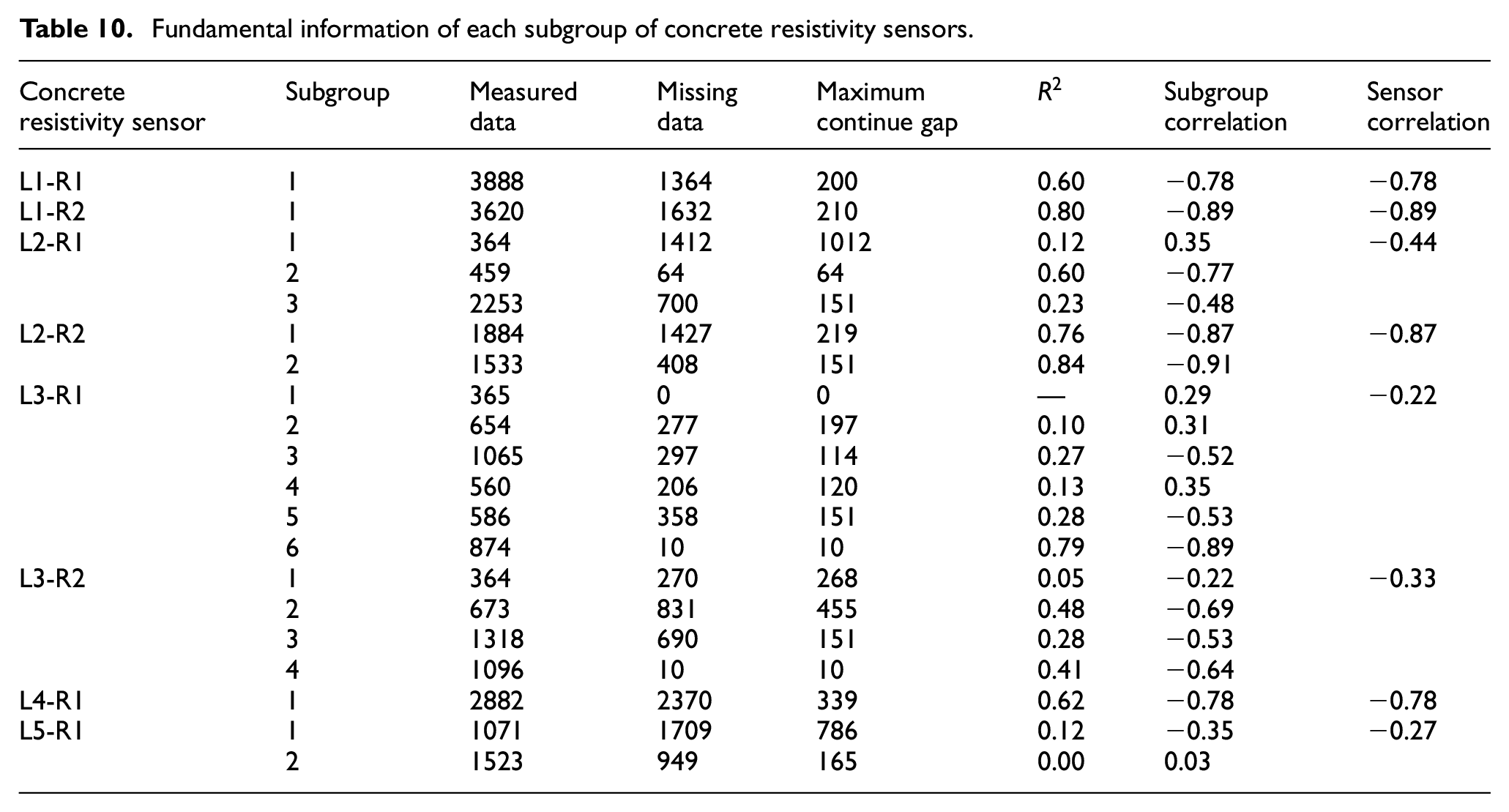
Once the subgroups for each sensor have been identified, the final part of stage D (Figure 3) is carried out. This part involves estimating the missing data for the subgroups using GLM models to complete the information for the resistivity sensors. For sensors where no subgroups were identified, the entire database of the sensor and the air temperature was used for the estimation of missing data. Table 10 also presents the subgroups obtained from the methodology, the amount of known and missing data, the largest continuous gap of missing data.
Table 10 also provides the
Data filling of the concrete resistivity sensors using pattern identification and GLMs for each sensor.
Sensitivity analysis of error propagation
A sensitivity analysis was conducted to evaluate the impact of the MAE results of Table 6 in the imputation of air temperature on the subsequent predictions of concrete temperature and electrical resistivity. Since air temperature is a key input in the imputation process, it was necessary to assess how uncertainties in its estimation propagate through the model and affect the predicted values for other variables.
Three scenarios were defined to simulate the potential impact of the MAE on the imputed air temperature: Scenario 1: The imputations of air temperature were increased by the MAE value of 3.51°C. Scenario 2: The original imputed air temperature was used as a baseline. Scenario 3: The air temperature imputation were decreased by the MAE value of 3.51°C. For each scenario, the Generalized Linear Model (GLM) was applied to predict the missing values of concrete temperature and resistivity. The differences between the predictions in Scenario 1 and Scenario 3 were compared to those in Scenario 2 (baseline) to quantify the impact of perturbations in air temperature on the predicted variables.
The sensitivity analysis demonstrates that the MAE of 3.51°C in the imputed air temperature has a minimal effect on the predictions of concrete temperature and resistivity, with average impacts of less than 1.5%. Table 11 presents the impact on the imputation of concrete temperature and concrete resistivity, calculated as the relative error with respect to Scenario 2 (baseline). This low sensitivity indicates that the model is resilient to uncertainties in air temperature imputations, supporting the validity and robustness of the proposed methodology. The slight asymmetry observed in the results suggests that further investigation could be conducted to better understand the model’s sensitivity to variations in lower temperature ranges, but these findings do not compromise the overall reliability of the results.
Impact of air temperature imputation errors on concrete temperature and resistivity predictions.
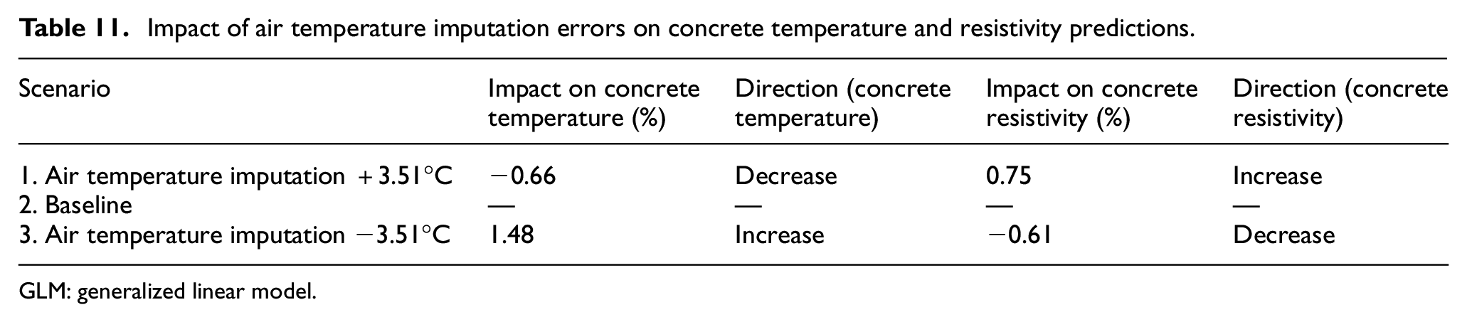
GLM: generalized linear model.
Conclusions
The present research addresses the challenge of missing data in the durability performance monitoring of RC structures using SHM systems. The proposed methodology employs a combination of feed-forward neural networks, generalized linear models, and pattern recognition techniques to impute missing data in air temperature measurements as well as in concrete resistivity and temperature sensors.
The scientific value of this study lies in the significant expansion and improvement of a preliminary methodology presented by the authors. 10 While the previous work was limited to a single year of data for a single resistivity and temperature sensor and focused on filling small data gaps of up to 61 days, this articleintroduces a more robust approach. By incorporating over fourteen years of sensor data and integrating air temperature as an additional input for data imputation, the present study demonstrates a more comprehensive and accurate methodology capable of filling longer data gaps. This is the first study, to the best of the authors’ knowledge, to apply such an imputation methodology for missing data in resistivity sensors within SHM systems.
The results demonstrate that the methodology is particularly effective for sensors with strong correlations between temperature and resistivity (absolute Pearson’s correlation value greater than 0.7) and high
Despite these advances, some limitations remain. The methodology relies heavily on the correlation between temperature and resistivity, which can be problematic in scenarios of concrete deterioration, where this relationship may break down. This limits the effectiveness of the approach in certain deteriorated conditions. Furthermore, the use of GLMs proved to be effective in subgroups with high correlation, but less so in groups with lower correlation values, suggesting the need for future research into more advanced computational models that do not depend solely on correlation.
Pattern recognition allowed the identification of subgroups with similar behaviors, improving Pearson’s correlation and missing data estimation. However, with only 43.4% of the estimated data achieving a strong correlation with the measured data, there is still room for improvement. Future studies could explore the application of more sophisticated machine learning models or hybrid approaches that can address data variability more effectively, particularly in regions with high uncertainty.
Footnotes
Declaration of conflicting interests
The author(s) declared no potential conflicts of interest with respect to the research, authorship, and/or publication of this article.
Funding
The author(s) disclosed receipt of the following financial support for the research, authorship, and/or publication of this article: This work is financed by national funds through FCT—Foundation for Science and Technology, under grant agreement 2021.05862.BD attributed to the first author. Doi: ![]() .
.
This work was partly financed by FCT/MCTES through national funds (PIDDAC) under the R&D Unit Institute for Sustainability and Innovation in Structural Engineering (ISISE), under reference UIDB/04029/2020 (doi.org/10.54499/UIDB/04029/2020), and under the Associate Laboratory Advanced Production and Intelligent Systems ARISE under reference LA/P/0112/2020.
Ethics approval
Not applicable.
Consent to participate
Not applicable. This article does not contain any studies with human or animal participants.
Consent for publication
Not applicable.