Multiple-input,multiple-output modal testing of a Hawk T1A aircraft: a new full-scale dataset for structural health monitoring

Abstract

The use of measured vibration data from structures has a long history of enabling the development of methods for inference and monitoring. In particular, applications based on system identification and structural health monitoring have risen to prominence over recent decades and promise significant benefits when implemented in practice. However, significant challenges remain in the development of these methods. The introduction of realistic, full-scale datasets will be an important contribution to overcoming these challenges. This article presents a new benchmark dataset capturing the dynamic response of a decommissioned BAE Systems Hawk T1A. The dataset reflects the behaviour of a complex structure with a history of service that can still be tested in controlled laboratory conditions, using a variety of known loading and damage simulation conditions. As such, it provides a key stepping stone between simple laboratory test structures and in-service structures. In this article, the Hawk structure is described in detail, alongside a comprehensive summary of the experimental work undertaken. Following this, key descriptive highlights of the dataset are presented, before a discussion of the research challenges that the data present. Using the dataset, non-linearity in the structure is demonstrated, as well as the sensitivity of the structure to damage of different types. The dataset is highly applicable to many academic enquiries and additional analysis techniques which will enable further advancement of vibration-based engineering techniques.

Introduction

The unexpected failure of many types of structures – including bridges, buildings, aircraft, power infrastructure, and marine vessels – can be financially costly and can also a present severe set of safety risks. The field of structural health monitoring (SHM) aims to use data collected from a structure to detect the presence of damage, localise its position, categorise its type, assess its extent and predict the future life of the structure.^1–4

Vibration-based monitoring of structures is a highly informative process for examining engineering structures, which are often used for SHM. Modal characteristics are particularly useful for inferring structural properties; this is due to their sensitivity to both the global and local physics of the structure as well as their relatively low dimensionality. ⁴ In predominantly linear systems, damage (in the form of cracks and material failure) is often detectable as a local loss of stiffness, leading to a shift in the natural frequencies of the system. However, the presence of non-linearity can lead to both false positives and false negatives in the damage identification task. ⁵ The additional difficulty of discriminating between data from a structure in its normal condition – with potentially variable operating conditions^6,7– or in the presence of structural damage, is an ongoing challenge in SHM.

The development of robust methods for SHM requires meaningful, high-quality, openly available benchmark datasets. Furthermore, there is an urgent need to bridge the gap between simple laboratory structures and full-scale structures in service, since many existing datasets are either highly complex or overly simplistic: examples include civil structures (such as the Z24 road bridge ⁸ and LUMO lattice mast ⁹ ), individual components such as aerofoils,^10,11 or bench-top models with comparatively simple geometries.^12,13 Bridging the gap between these two levels of complexity this will require datasets which

• (1) Are sufficiently realistic to describe in-service engineering structures.

• (2) Are sufficiently complex that system identification is not trivial using current methods.

• (3) Contain data from a number of different conditions (including operating conditions and damage states).

In this article the authors present a new benchmark dataset for the purposes of SHM and system identification (SYSID). This dataset consists predominantly of force, acceleration and strain data collected from dynamic testing of a BAE Systems Hawk T1A aircraft. The work significantly extends a previous dataset collected by Haywood-Alexander et al.,^11,14 which considered only the starboard wing of the same aircraft. In addition to extending vibration testing of the both the undamaged and pseudo-damaged structure to the entire body of the aircraft, the current dataset also builds on the previous work by including data from multiple-input multiple-output (MIMO) testing, multi-site pseudo-damage tests, and data from actual damage induced by removing panels from the skin of the structure (Table 1).

Table 1.

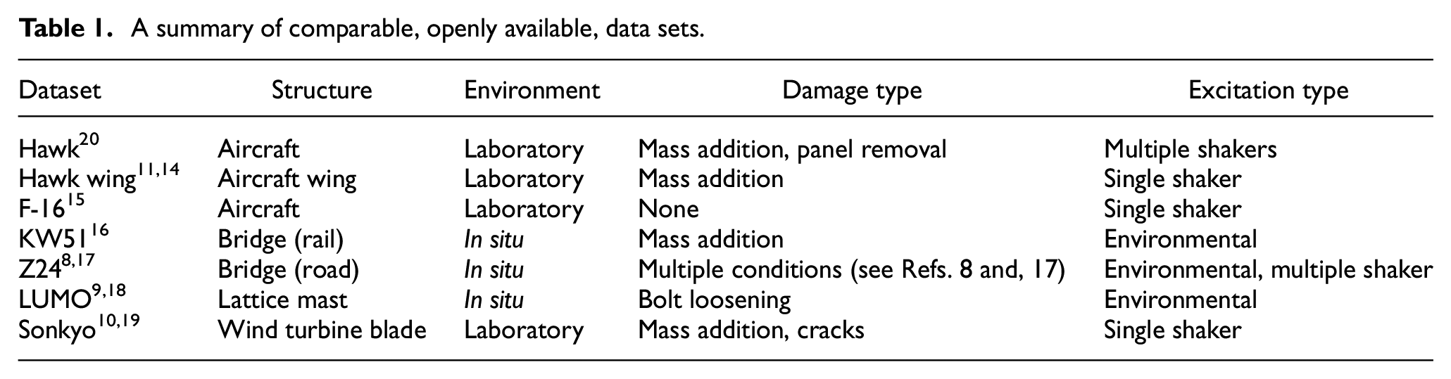
A summary of comparable, openly available, data sets.

Dataset	Structure	Environment	Damage type	Excitation type
Hawk 20	Aircraft	Laboratory	Mass addition, panel removal	Multiple shakers
Hawk wing11,14	Aircraft wing	Laboratory	Mass addition	Single shaker
F-16 15	Aircraft	Laboratory	None	Single shaker
KW51 16	Bridge (rail)	In situ	Mass addition	Environmental
Z248,17	Bridge (road)	In situ	Multiple conditions (see Refs. 8 and, 17)	Environmental, multiple shaker
LUMO9,18	Lattice mast	In situ	Bolt loosening	Environmental
Sonkyo10,19	Wind turbine blade	Laboratory	Mass addition, cracks	Single shaker

The dataset is freely provided with the intention that it might be used by others to develop new algorithms for structural dynamics. Access is facilitated via a Python interface (https://github.com/MDCHAMP/hawk-data) developed by the authors for both this dataset and the previous dataset by Haywood-Alexander et al.^11,14

The remainder of this article is structured as follows: first, the Hawk structure is described in detail. Second, the experimental work is described, including discussions of the testing regime, setup and hardware and acquisition and control. A further section describes the dataset itself. Finally, the challenges presented by this new dataset are explored, including SYSID and SHM. The principal contributions of this work are as follows:

• A full-scale MIMO vibration test of the BAE Systems Hawk T1A aircraft is presented as a new benchmark dataset.

• The dataset includes broadband excitation data from five locations on the Hawk, which was instrumented with over 140 sensors.

• The dataset comprises over 200 test conditions including different excitation signals and amplitudes, as well as comprehensive damage simulations.

• The entire dataset is made freely available alongside with a convenient Python interface that enables users to work with a subset of the data as required.

Structure

The structure presented in this article is a BAE Systems Hawk T1A (‘the Hawk’) that was donated to the University of Sheffield by the Defence Science and Technology Laboratory. The Hawk is housed at the Laboratory for Verification and Validation (LVV) within the university; it is a decommissioned aircraft previously used for advanced training by the British Royal Air Force. Structurally, the airframe of the aircraft is largely complete; however, the engine, certain wing flaps, the cockpit canopy and various other components have been removed. The aircraft is positioned resting on its wheels on the ground. A full set of technical drawings is not available.

Figure 1.

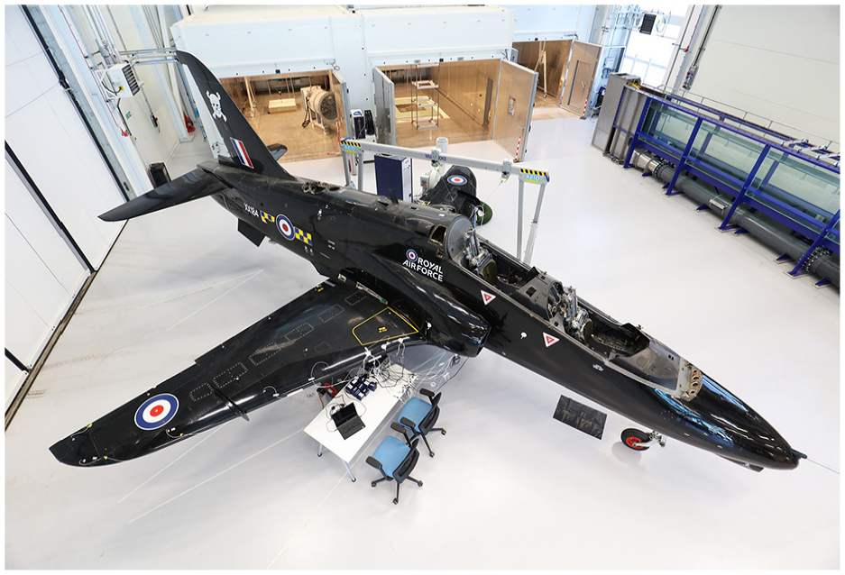
The Hawk at the laboratory for verification and validation.

Experimental work

Details of the experimental work are presented in this section. First, the experimental setup and hardware are described, followed by details of the testing regime. Finally, the acquisition and control of the input force are discussed. A full set of schematic diagrams summarising the placement of accelerometers, shakers, fibre-Bragg grating (FBG) strain gauges and damage locations are given in Figures 2 to 6 to complement this section.

Figure 2.

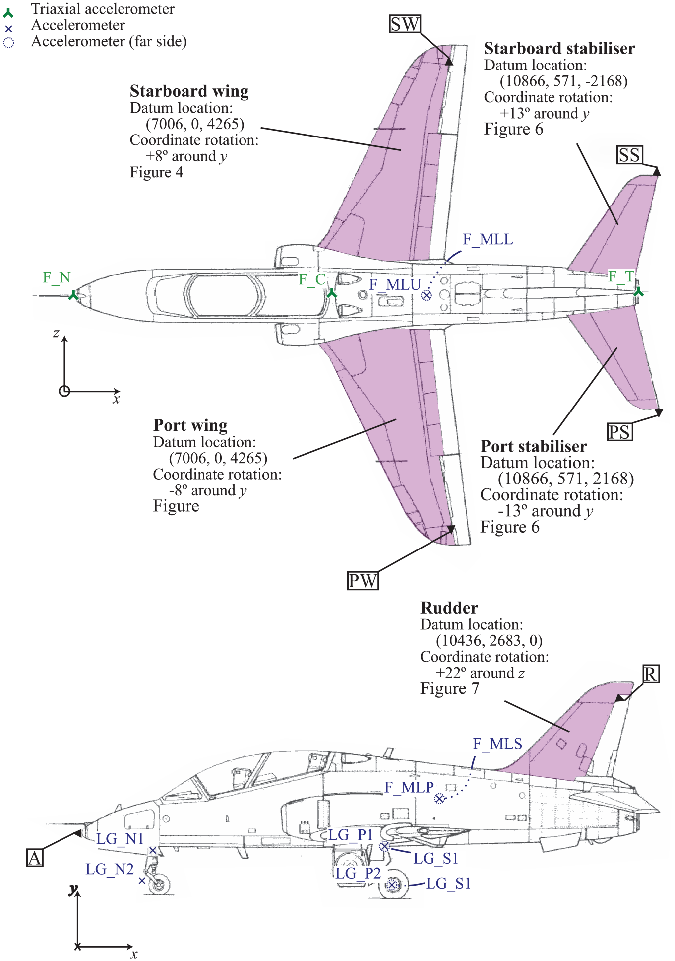
Summary sensor placement sketch for the Hawk, showing the locations of the nearside, farside and triaxial accelerometers on the main chassis. Also shown are the locations of the datums (SW, SS, PS, and PW) relative to the global datum, A. The substructures highlighted in magenta are detailed in Figures 3 to 6. The diagram is not shown to scale – for precise locations, refer to the dataset. ²⁰

Figure 3.

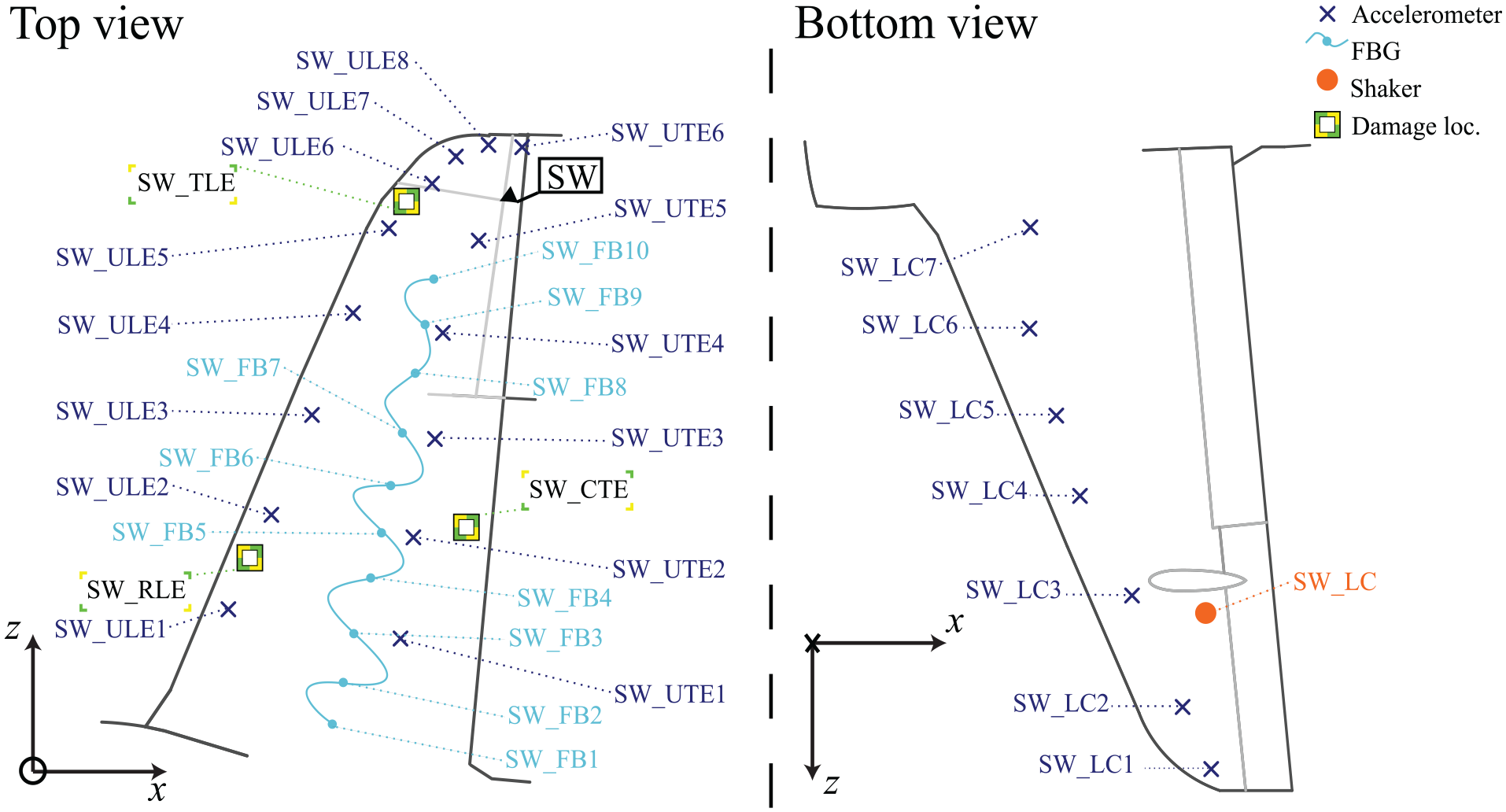
Schematic diagram for the starboard wing, showing the location of the accelerometers, FBGs, shakers, and pseudo-damage. Not to scale.

Figure 4.

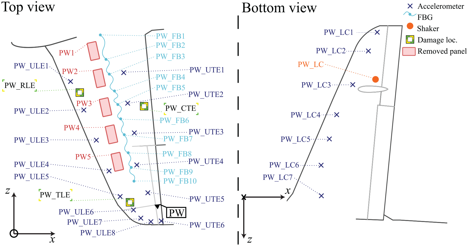
Schematic diagram for the port wing, showing the location of the accelerometers, FBGs, shakers, pseudo-damage and removed panels. Not to scale.

Figure 5.

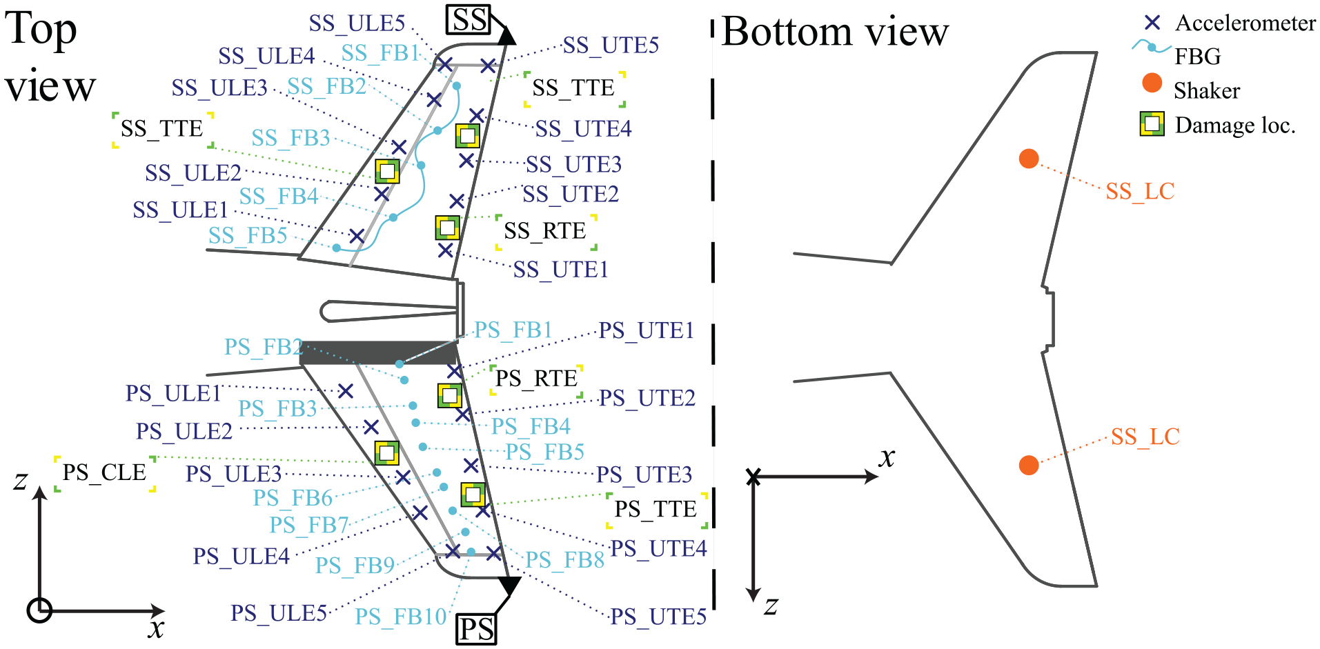
Schematic diagram for the stabilisers, showing the location of the accelerometers, FBGs, shakers and pseudo-damage. Not to scale.

Figure 6.

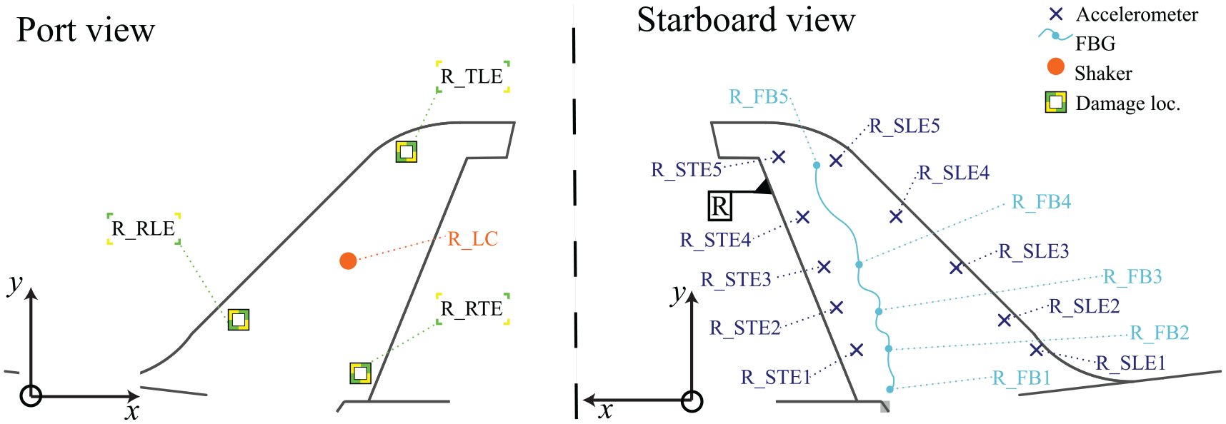
Schematic diagram for the rudder, showing the location of the accelerometers, FBGs, shaker and pseudo-damage. Not to scale.

Setup and hardware

Five types of sensor were used in these tests: accelerometers, FBG strain gauges, force transducers, a resistance temperature detector (RTD) and a microphone. The force transducers measured the excitation forces from the shakers, the accelerometers recorded the acceleration response and the strain gauges recorded the strain. The ambient temperatures were recorded using the RTD and a triaxial accelerometer recorded ground vibrations. All of these measurements were recorded in the time domain. Ambient noise was also recorded using a microphone; for privacy reasons this was not recorded in the time domain – a Fourier transform of these data was recorded instead. An image of the Hawk during instrumentation is shown in Figure 7.

Figure 7.

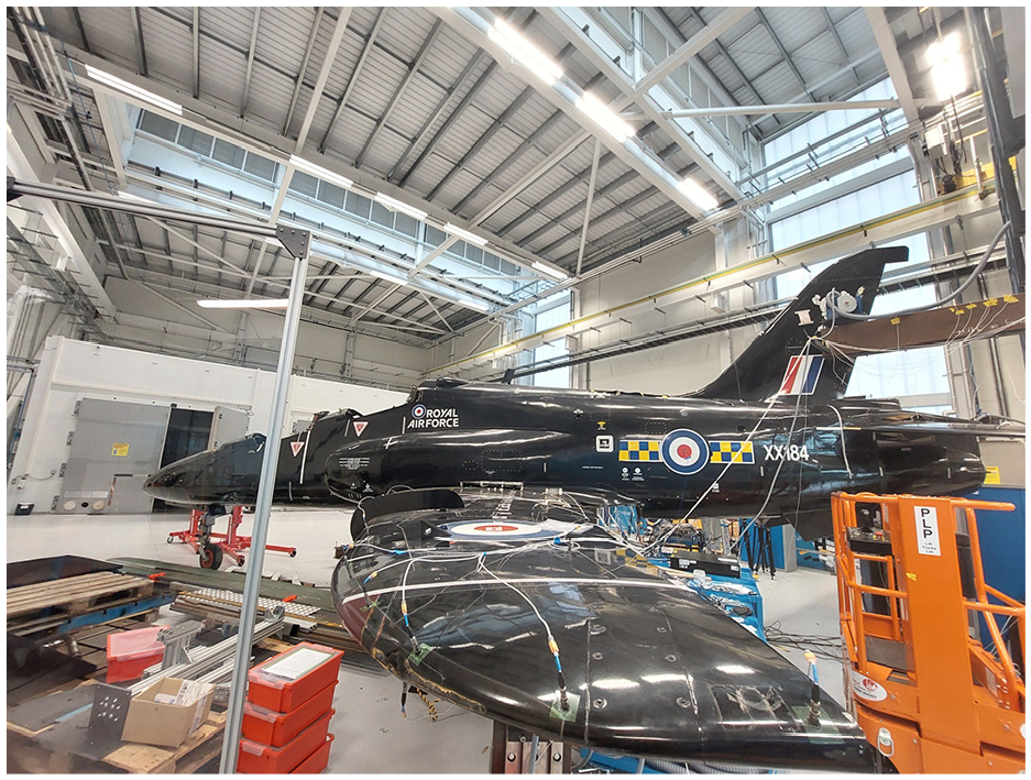
The port wing of the Hawk during instrumentation.

The electrodynamic shakers were positioned to excite each wing, each stabiliser and the rudder. This was to ensure that a strong dynamic response could be recorded across the whole structure. Their exact locations were guided by limitations of the structure (such as the need to avoid exciting near the landing gear). Tira TV 51140-MOSP modal shakers were used in conjunction with BAA 1000 amplifiers. The force transducers were PCB Piezotronics 208C02s, with a nominal sensitivity of 11,241 mV/kN.

To measure the structural response, PCB Piezotronics accelerometers were used with a nominal sensitivity of 10 mV/g. When converting voltage readings to acceleration values, the sensor-specific sensitivities (contained within the metadata ²⁰ ) were used. A set of triaxial accelerometers were placed at the nose, cockpit and tail of the Hawk fuselage; PCB Piezotronics accelerometers were used with a nominal sensitivity of 100 mV/g. A set of four uniaxial PCB Piezotronics accelerometers, also with a nominal sensitivity of 100 mV/g, were placed on the fuselage midpoint on the top, bottom, port and starboard sides. Pairs of these sensors were also placed on each landing gear; one above the hydraulic suspension and one on the axle of the wheel. A total of 85 accelerometers were placed on the Hawk.

FBG strain gauges were mounted along the length of each wing, as well as along each stabiliser and up the rudder. Ten measurement locations were placed on each wing, and on the port stabiliser. A single FBG strain gauge was shared between the rudder and the starboard stabiliser, meaning that five measurement locations were available on each of these substructures. The precision of the strain gauges was 1με and their measurement length was 10 mm; on a large surface such as the Hawk skin these can effectively be considered as point measurements.

One PCB piezotronics triaxial accelerometer, with a nominal sensitivity of 100 mV/g, was placed on the ground. A microphone was placed under the fuselage of the Hawk to record any significant ambient noise. The microphone was a GRAS 46AE with a precision of 0.08 dB. The RTD used was an RS PRO PT100 sensor and was accurate to 0.1°C. Exact sensitivities of all sensors are available as part of the dataset record at Wilson et al. ²⁰

The coordinate locations for the sensors were measured on the structure itself where possible; these were measured from local reference points on each surface. Despite some difficulties in measuring distances across curved surfaces, the location of these points is considered sufficiently accurate for SYSID. The global datum was taken from the tip of the nose (labelled ‘A’ in Figure 6) of the Hawk. The global measurements, including the coordinates of the various reference points, were measured from drawings of the Hawk, which was scaled to a particular reference length on the real structure. The coordinates shared as part of the dataset are intended for use in visualisation of the structure only; more advanced measurement techniques would be required to derive a set of fully accurate coordinates. Most sensors on the structure were aligned along a particular coordinate axis. Wherever there was a significant deviation in this direction, this is noted in the data record. All sensor coordinate data are available in Wilson et al. ²⁰

The landing gear tyres were inflated to a pressure of nine bar prior to testing. Following a period of downtime in the LVV from 10th to 25th August 2023, the tyres were repressurised to this value on 29th August 2023.

Testing regime

The experimental work was carried in five phases. The first phase concerned the acquisition of data to fully describe the normal, undamaged condition of the Hawk. The aircraft was excited by signals with a range of amplitudes, enabling the identification of any amplitude-dependent non-linearities. Input excitation signals were designed as white noise and pink noise signals. For all tests, the excitation bandwidth was 5–256 Hz and the sampling rate was 2048 Hz.

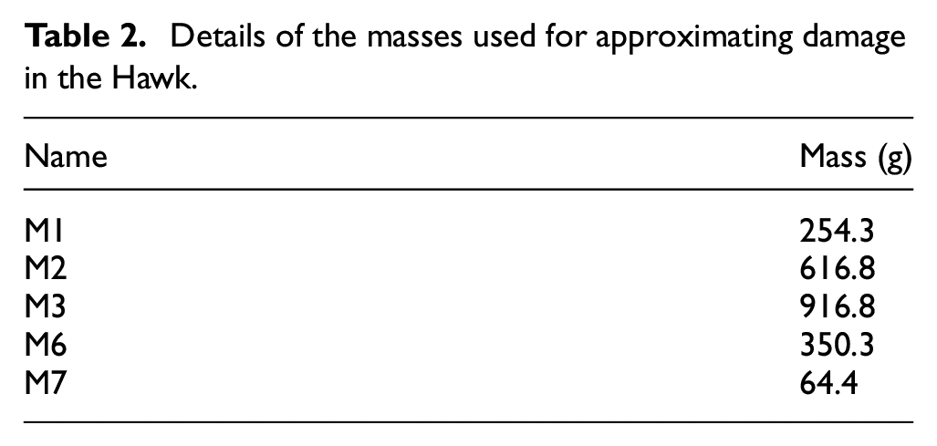
Following the undamaged tests, the Hawk was tested in a range of single-site damage scenarios. The damage scenarios considered in these tests were limited to interventions that would not permanently affect the integrity of the structure. Other conditions, such as bolt loosening or the introduction of cracks were therefore not investigated. Pseudo-damage was introduced to the structure by the addition of weights of varying mass at a range of locations; mass addition has a similar impact on the dynamic response of a system to loss of stiffness caused by true damage, and can therefore be used in non-destructive demonstrations such as these. ²¹ The masses were attached to the surface of the Hawk by suction cup. Details of the masses used are given in Table 2. Damage locations are presented in the schematic diagrams shown in Figures 3 to 6. White noise excitation was used for these tests, where the excitation bandwidth was 5–256 Hz and the sampling rate was 2048 Hz. A range of excitation amplitudes were used, corresponding to those used in the first testing phase.

Table 2.

Details of the masses used for approximating damage in the Hawk.

Name	Mass (g)
M1	254.3
M2	616.8
M3	916.8
M6	350.3
M7	64.4

The third phase of testing entailed excitation of the structure in its undamaged condition using odd random-phase multisine (ORPM) excitation. This is a popular input design method to enable non-linear SYSID in the frequency domain. The excitation profile contains a random selection of odd-frequency sine waves; leakage into the response of other frequency content can then be treated as an indicator of non-linearity in the structure. ²² The ORPM tests were carried out with the Hawk in its undamaged condition, and also with some single-site mass additions. Initial ORPM tests were conducted in a single-input multiple-output (SIMO) configuration, considering each input location separately, with following tests carried out as previously in a MIMO configuration.

The fourth phase of testing investigated the response of the Hawk to multisite damage. The structure was excited using white noise signals in the range 5–256 Hz, and the sampling rate was again 2048 Hz. The same masses and locations as were used in the single-site damage tests were employed here. Up to three masses were positioned on the structure at any one time.

The final phase of testing involved a series of actual damage-state tests where surface panels were removed from the port wing of the Hawk. The panels were arranged in a line along the length of the wing; five panels were identified for the tests and were labelled PW1–PW5. The panel removal tests were carried out at the end of the testing to avoid the impact that the removal and reattachment of any panels may have on the response of the structure in other tests. Only one panel was removed at a time, and for each scenario, the structure was excited with white noise signals at three different amplitude levels.

The full experimental campaign comprised 216 individual tests. For the sake of brevity, the full list is not tabulated here. The interested reader is directed to the dataset at ²⁰ for the full downloadable tabular record of test conditions; a hierarchy of the test structure is also illustrated in Figure 8.

Figure 8.

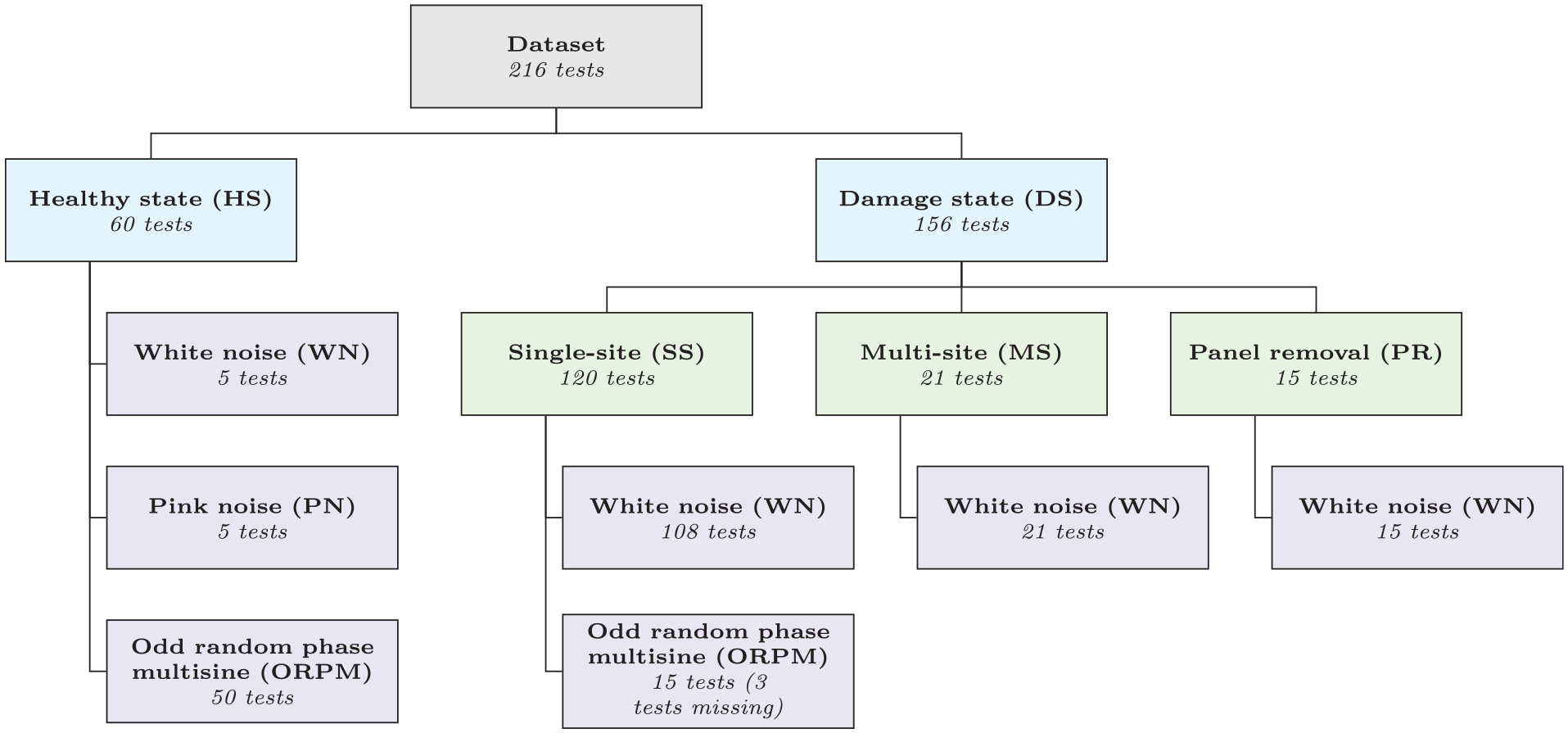
A graphical illustration of the structure of the dataset.

Acquisition and control

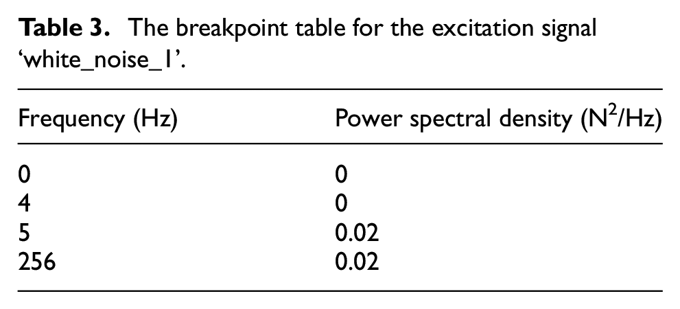
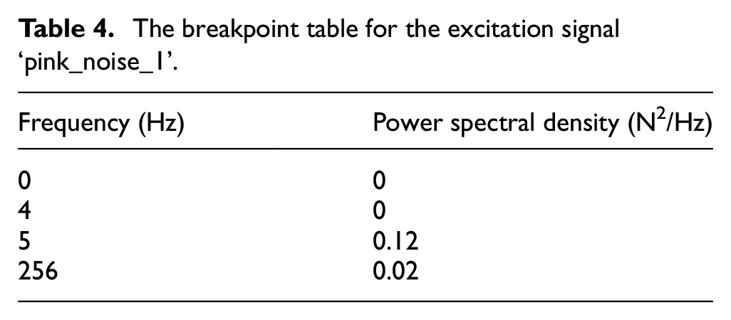
The majority of testing on the Hawk was carried out using random excitation, with white noise and pink noise signals used. The spectral densities of the input signals were pre-determined using ‘breakpoint’ tables. These tables define a rectangular or trapezoidal spectral density profile (for white and pink noise respectively) in the frequency domain for each shaker. The highest input amplitude was limited by the maximum safe level of excitation that could be applied to the Hawk via stinger, and the testing amplitudes were reduced linearly from these upper bounds. In total, five excitation levels are defined for both white and pink noise excitations.

Sample breakpoint tables for white noise and pink noise excitation are given in Tables 3 and 4. The breakpoint tables were resampled 8192 times to generate an amplitude ‘mask’ across the full bandwidth (up to 2048 Hz). For a full description of all breakpoint tables and input signal metadata, the reader is directed to the dataset record. ²⁰

Table 3.

The breakpoint table for the excitation signal ‘white_noise_1’.

Frequency (Hz)	Power spectral density (N 2 /Hz)
0	0
4	0
5	0.02
256	0.02

Table 4.

The breakpoint table for the excitation signal ‘pink_noise_1’.

Frequency (Hz)	Power spectral density (N 2 /Hz)
0	0
4	0
5	0.12
256	0.02

It should be noted here that the signals used are generally lower in amplitude than those used for the starboard-wing tests by Haywood-Alexander et al. ¹¹ This is due to the MIMO nature of this testing campaign; overall, a greater total excitation energy is supplied compared to a single-shaker setup. Furthermore, excitation was additionally applied to substructures of the Hawk tailplane (stabilisers, rudder) that are likely to have a dramatically lower stiffness than the wings, requiring less input energy for a similar signal-to-noise ratio.

The time-domain drive signals for each input shaker were generated by an iterative procedure. For each of the five shakers, a unique drive signal was created by generating a random summation of sine waves, each of which was assigned a random phase. The initial amplitude mask (in the frequency domain) could then be generated by multiplying the breakpoint table by an initial value of 0.01, which provided a conservative point at which to begin iterating the drive signals. Each shaker was driven with its corresponding drive signal and the output measured at the load cell was compared to the target power spectral density (PSD) defined by the breakpoint table. The quotient of the two was then used as a multiplier to update the drive signal for the next iteration. This process was iterated until the error between the measured and target PSDs met a defined tolerance – set to 4% for these tests – for all shakers, at which point, the spectral gain mask was stored for each shaker.

The drive signals were then generated for each shaker according to the spectral gain masks. The spectral gain masks were resampled in the frequency domain to differing lengths by linear interpolation to allow for variable test periods to be specified. This would introduce some error on the desired excitation, which could be captured by interrogating the measured excitation signals for each test. New spectral drive masks were generated if the structure was modified between tests (such as by adding a pseudo-damage mass) or at the beginning of each test session to account for the effects of any variations on the structure.

For the ORPM tests, a mask of ones and zeros was generated to accept the odd spectral content and reject the even content. This was used as an additional multiplier when generating the drive files. 50% of the odd frequency content was retained for each iteration of the ORPM tests.

Dataset

Overall, 216 tests were conducted during the campaign, each comprised of 139 individual sensor channels with an average of 10 repeats per test. The raw size of the collected dataset exceeds 500 GB, far in excess of most users’ capacity to load it into memory. A graphical illustration of the structure of the dataset with respect to the testing carried out is provided in Figure 8.

The Hawk full-structure dataset is packaged in the widely used hierarchical data format (.hdf5). The .hdf5 format allows data and metadata to be stored concurrently and facilitates lossless data compression. Many software packages are available for opening and exploring .hdf5 files and programmatic access is implemented in most popular programming languages.

In order to further facilitate simple and practical access to the data, a simple interface has been created in the Python language. The Python interface (available at github.com/MDCHAMP/hawk-data) automatically handles the downloading and storage of the Hawk data from the centralised repository ²⁰ ensuring that the data are up to date and avoiding generation loss by repeated sharing. Data are accessed programmatically meaning that only data that is required by the user is downloaded. The API first checks for local versions of the files and, if they do not exist, accesses the data from the central repository, comparing the MD5 hash to ensure the data is up to date. Note that use of the Python interface is not required in order to obtain the data, it is only provided to simplify the process for users who require such functionality.

In order to serve only the data that are required to the user, the whole dataset is divided into discrete units. This is achieved by leveraging the hierarchical nature of the .hdf5 file format and using external links to connect a number of separate .hdf5 files to a single .hdf5 header file. Data files are atomised on a per-test basis, including all repeats and metadata. Dividing the dataset in this way allows it to be distributed in single-test files, each around 1 GB in size (rather than a single compressed record of around 250 GB). Packaging the data in this way drastically lowers the required disk footprint for users who only require a subset of the test conditions for benchmarking and analysis.

Additionally (as in Haywood-Alexander et al. ¹¹ ), the dataset has been compiled in a self-describing format. Self-describing datasets package pertinent metadata alongside raw sensor output data in order to create a data record that does not require the user to have detailed knowledge of the test campaigns in order to use the data. In the context of the Hawk, full structure test metadata (i.e., signal name, sensor, sensor type, sensitivity, sensor location, units and test conditions) are stored alongside each channel in a hierarchical format. For a more complete description of which metadata are available, the interested reader is directed to the usage examples on the data repository. ²⁰

Dataset challenges

In section ‘Introduction’, the authors argued that bridging the gap between SHM of laboratory and full-scale structures requires the use of realistic, complex datasets with data from a number of different conditions. It is hoped that the dataset presented in this article will be of interest to a wide range of researchers with a shared interest in understanding full-scale dynamic systems. In this section, some open research challenges that the dataset highlights are discussed. These challenges pertain to the practicalities of working with large datasets, SYSID of a complex structure, and SHM. Following each of these subsections, the key challenges are enumerated for ease of reference.

In order to visualise some salient aspects of the Hawk dataset, several frequency response functions (FRFs) are computed here in Figures 9 to 14. However even these simple analyses represent a non-trivial challenge for the Hawk dataset. Well-established methodologies can present challenges on large-scale datasets. In the context of the Hawk aircraft, a natural way to characterise the (predominantly) linear dynamics is through the lens of modal analysis. ²³ In the MIMO setting, the FRF matrix can be estimated from the measured input-output data. For a linear system in the frequency domain, one has

$$Y\left(\omega \right)=H\left(\omega \right)X\left(\omega \right)$$

(1)

where H is the MIMO FRF, and X and Y are the Fourier transforms of the input and output data respectively. Post-multiplying the above by the conjugate transpose of X and taking expectations gives

$$S_{xy}\left(\omega \right)=H\left(\omega \right)S_{xx}\left(\omega \right)$$

(2)

where S _xy is the cross-spectral density of the input with the output and S _xx is the auto-spectral density of the output. The linear Equation (2) can thus be solved for H at each frequency line. Attempting to solve the above for many input and output channels is likely to be poorly conditioned numerically and lead to corruption and artefacts in the identified FRF. In the present work, FRFs for visualisation are computed via a short-time Fourier transform (STFT) with a Hann window, a segment length of 16,384 and an overlap of 8192. The resulting linear system is solved in the least-squares sense by taking the inner product over the number of segments in the STFT.

Figure 9.

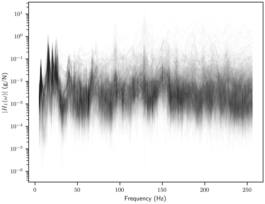
FRF magnitudes (from every accelerometer channel) superimposed for the white noise healthy state test at amplitude level 5.

Figure 10.

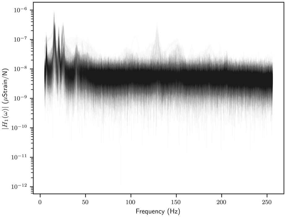
All FBG strain FRF magnitudes superimposed for the white noise healthy state test at amplitude level 5.

Figure 11.

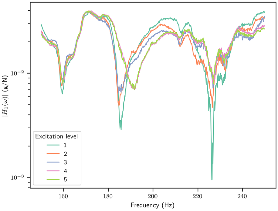
Cropped FRF magnitude from starboard wing shaker (SW_LC) to lower starboard landing gear (LG_S2) depicting non-linear hardening.

Figure 12.

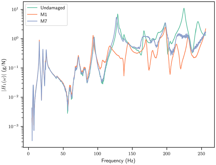
FRF magnitude from port wing shaker to PS_ULE5 in the presence of damage at PW_TLE (amplitude level 5).

Figure 13.

FRF magnitude from starboard stabiliser shakerto SS_UTE3 in the presence of damage at SS_TTE (amplitude level 5).

Figure 14.

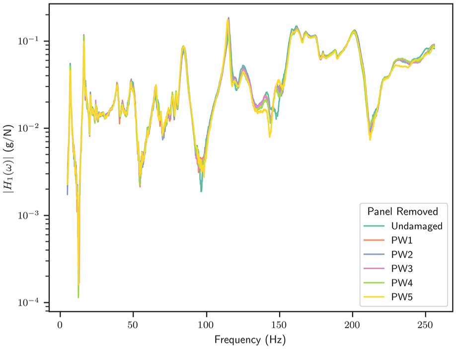
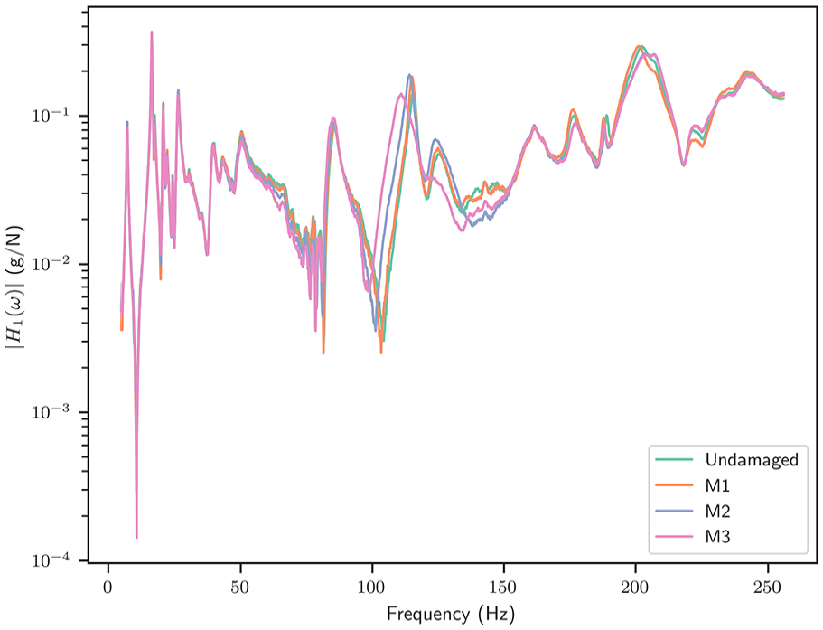
FRF magnitude from port wing shaker (PW_LC) to PW_ULE3 during the panel removal tests (amplitude level 5).

Large datasets

This dataset represents a comprehensive set of testing which may be carried out on a structural dynamic system. Inevitably, the testing of full-scale structures across a range of conditions gives rise to relatively large datasets, which may not be easily analysed on a local computer due to limitations in memory. As data-driven approaches to SHM become adopted more widely in industrial settings, the necessity of handling datasets of this scale will grow. In the context of an academic research environment, it is worth highlighting that as methodologies are developed, this context should be taken into account. The practicality of using already-established algorithms in the context of large datasets also needs to be evaluated.

Additionally, as the size of these datasets increases, reliance on ad hoc human interpretation of the data becomes harder and the need for further levels of automation in analysis will increase. For example, inspecting Figure 9, it is clear that the complexity of a structure such as the Hawk aircraft is very high and direct observations (even from a skilled operator) may be limited. In order for these techniques to be practical in industrial settings, operators need to be able to check, in a realistic timescale, that the data are being collected as expected. The development of practical workflows and the implementation of automated checks presents an open challenge. The key challenges can thus be summarised:

• Challenge 1. Using existing and new SYSID algorithms on large datasets in realistic time frames.

• Challenge 2. Aiding (or reducing the reliance on) operator interpretation when collecting large datasets.

System identification

It is envisioned that the Hawk dataset will provide a meaningful testbed for identification algorithms in the context of structural dynamics. For such dynamics analyses, it is often necessary to determine the underlying properties of the dynamic system (e.g., a representative set of governing differential equations) from the available data. This dataset presents a number of challenges to researchers in this area.

It is difficult to develop accurate models of large, built-up structures (such as this aircraft) owing to the richness of the dynamics involved. The dataset itself is generated using MIMO tests, which only increase the quantity of data in comparison to SIMO, and so can require more care in the signal processing.

In dynamical systems theory, it is generally assumed that a system is governed by a set of unknown partial differential equations which cannot be directly determined, and that have complex and unknown boundary conditions. The structure comprises components and subsystems, each of which have varying dynamic properties. These parts are assembled into the full structure in a manner which requires modelling of jointed interactions – an open area of fundamental research.^24–26

Figures 9 and 10 show the combined data recorded from the structure to interrogate the form of the FRFs for the acceleration and strain sensors, respectively. The figures give an idea of which resonances are present in the majority of channels by plotting each individual FRF with 50% transparency. Darker peaks represent global resonances (where many sensors have large responses) and more faint peaks correspond to more localised resonances (only present in a small number of sensors). While behaviour can be distinguished in the FRFs which may be attributed to global modal behaviour in the low-frequency region, the full picture is far more complicated. Since the structure contains many thin panels, a global modal behaviour is difficult to resolve. It can therefore be expected that alternative methods that combine deterministic and statistical analyses such as hybrid statistical energy analysis (SEA), ²⁷ will be required.

Figure 11 depicts a subset of the frequency lines from the FRF of the starboard wing shaker to the lower section of the landing gear on the starboard wing. Here, a further challenge becomes apparent. The FRF in certain regions of the frequency range can be seen to exhibit strong dependence on the excitation amplitude. This dependence is one indicator that the dynamics of the structure are not well approximated by linear theory. The behaviour observed in 11 shows some drift resonant peaks with increases in amplitude which may be associated with non-linear hardening behaviour in those resonances (and anti-resonances). The presence of non-linear dynamics in aerospace structures is well known in the literature, for example see a previously published dataset ²⁸ where testing is carried out on an F-16 aircraft. The identification of non-linear systems with many degrees of freedom remains a challenge and this dataset adds to the utility of ²⁸ by providing a MIMO test case and an extended sensor network covering the full structure. It should be noted that the complexities previously discussed regarding the mid-frequency region continue and may require the utilisation of non-linear forms of SEA, for example Spelman and Langley. ²⁹

One common purpose of system identification is to update or validate existing physics-based models of the structure of interest; model calibration and validation are critical to ensuring the accuracy and reliability of a predictive model and model updating is applicable as a damage inference problem. Uncertainty quantification for physics-based models, particularly in the face of epistemic uncertainty as in this dataset,^4,30 is a major challenge. The lack of a high-quality numerical model, as is common with legacy infrastructure, increases the applicability of this challenge.

In the context of a built-up, multi-component structure such as the Hawk, the idea of hierarchical validation offers potential solutions to a range of issues concerned with model validation,^31,32 where relevant challenges would include how to combine datasets collected on components and subsystems of a more complex overall object. There is an opportunity to investigate model updating in this hierarchical context by using this dataset in combination with the previously presented starboard wing data. ¹¹

The challenges relating to the Hawk dataset in SYSID are summarised below:

• Challenge 3. Developing accurate models of large, built up structures using MIMO data.

• Challenge 4. Modelling the dynamic properties of structures with jointed subsystems.

• Challenge 5. The identification of global modal behaviour.

• Challenge 6. The identification of non-linearities within the system.

• Challenge 7. Uncertainty quantification and physics-based model updating in the face of epistemic uncertainty.

• Challenge 8. Hierarchical validation, in conjunction with the previous dataset.

Structural health monitoring

As previously stated, the principal purpose of the Hawk dataset is to provide a meaningful benchmark for SHM in aerospace structures. It is intended that the presented dataset is able to function as a useful tool to bridge the gap between small-scale laboratory experiments and complete operational systems. The level of system complexity seen in this dataset greatly complicates the application of many SHM approaches. Opportunities exist to extend existing and develop new techniques spanning the all levels of Rytter’s hierarchy barring remaining life prognosis. ¹

Various levels and types of (pseudo-)damage have been simulated to provide a number of scenarios under which methods may be tested. The addition of masses has been conducted in the same manner as shown in Haywood-Alexander et al., ¹¹ this point is important as it allows the evaluation of methods from a population-based structural health monitoring viewpoint where transfer learning may be applied between the two alternative sensing and excitation setups. The effects of these added mass simulated damages are illustrated in Figures 12 and 13 for the cases where damage has been simulated on the port wing and starboard stabiliser, respectively. Both figures show pronounced effects at higher levels of added mass (mass references in figure legends refer to Table 2). It is expected that detection of these damage scenarios should be achievable on the basis of the response in the higher-frequency ranges.

Of particular interest is the effectiveness of methods using only the strain data or methods which seek to perform classification or estimation of damage extent. It would be especially desirable if these quantities could be transferred between this test dataset and that previously published on only a single wing. ¹¹

A further challenge is the case of panel removal. Such a case is shown in Figure 14, where FRFs are shown for panels removed from the port wing of the aircraft. The effect of the panel removals is, at least visually, significantly harder to detect than that of the added masses and should be considered as a more meaningful challenge with respect to the testing of any SHM methodology.

If SHM technologies are to see widespread adoption, they must consider whether it is practical to collect required data for different algorithms during the operational life of the structure. There exists a distinction between what data would be available in a laboratory or development setting and what could be practically collected in service. Installing a comprehensive network of accelerometers on an aircraft for use in flight is a concept that presents many practical difficulties. It is for this reason that FBG data were included in this dataset, in addition to the accelerometer data. Alternative sensing techniques, such as FBG sensors, may provide more viable routes to in-service monitoring of structural vibrations. However, each sensing modality comes with its own restrictions and limitations. For example, in the case of the FBG data, a much lower signal-to-noise ratio is present, which may be observed when comparing Figure 10 to Figure 9. Performing SHM with this sparser, noisier data present a greater challenge than with the accelerometer data.

Finally, an open question remains concerning the change in available data between the ‘training’ phase of an SHM algorithm and that which is used in ‘testing’ (i.e., practical usage). This can be summarised as ‘Should “higher quality” data be used during algorithmic development with a view to adapt to the data available in use or should only operationally available data be used?’. The picture is complicated even further if a population-based approach ³³ is taken. It is hoped that the data set presented here can be used to further explore this question in the future.

Dataset challenges in SHM are summarised below.

• Challenge 9. Detecting and classifying pseudo-damage using the entirety of the available data.

• Challenge 10. Detecting and classifying pseudo-damage using subsets of the available data.

• Challenge 11. Detecting and classifying panel removal with any amount of the available data.

• Challenge 12. Detecting and classifying pseudo-damage with exclusively the FBG data.

• Challenge 13. Establishing the extent to which higher-quality data is useful in the training phase, when only lower quality data is available during operation.

Conclusion

This article presents a new comprehensive dataset for SHM, acquired from a BAE Systems Hawk T1A. The intention of the dataset is to provide a benchmark for the development of vibration-based SHM and SYSID methods on a full-scale aerospace structure, with the benefit of laboratory testing conditions.

The key details of the experimental work carried out to acquire the data have been described. Representative sections of data have been presented to highlight damage sensitivity, non-linearity and strain responses of the structure. These examples were presented to indicate the potential applications and challenges of the dataset in future research work.

The key challenges that are foreseen based on this dataset relate primarily to SYSID and SHM. Here, the large scale of the dataset, the significant complexity in the dynamics (including non-linearity) and the use of strain measurements were highlighted as future challenges for the research community to address.