
Abstract
This study introduced a framework that facilitates bridge diagnostic and prognostic evaluations and related visualizations, leveraging building information modeling (BIM) techniques and data-driven structural health monitoring. Diagnostic and prognostic algorithms are proposed and able to provide intuitive and accessible structural insights via three-dimensional visualizations supported by the BIM techniques. Through the data communication channel established, virtual model information was successfully embedded into the bridge health evaluations, emphasizing the contribution of BIM techniques for data analysis. The proposed algorithms were applied to a case study of a reinforced concrete bridge. Strain distribution along the bridge deck was mapped in the 3D virtual model, which was able to precisely identify the critical location for potential damage. The residual fatigue life of different parts of the bridge deck was estimated and visualized by considering the main effects of traffic loading, exhibiting good alignments with the diagnostic results. The proposed framework is able to provide understandable and actionable structural information for stakeholders, facilitating the timely identification of structural issues and long-term planning of maintenance schedules.
Keywords
Introduction
Structural health monitoring (SHM) systems, employing an array of sensors such as strain gauges (SGs), accelerometers, and thermometers, offer continuous, real-time, and objective monitoring of the behavior of infrastructures. With the advancement of sensor technologies, SHM systems have gained increasing recognition in the field of bridge health monitoring and management, where diagnostic and prognostic evaluations constitute two important components of bridge SHM data analysis and interpretation, working collaboratively to ensure structural integrity and longevity. In detail, diagnosis involves the interpretation of monitoring data to detect, locate, and characterize any damage or deterioration in bridge structures. Prognosis, extending beyond diagnosis, involves predicting the future condition of the bridge based on current diagnostic data and the historical performance of the structure. A number of bridges, such as the Tsing Ma Bridge, 1 the Golden Gate Bridge, 2 and the Akashi-Kaikyo Bridge, 3 have adopted SHM systems for efficient and labor-saving health monitoring.
In the field of current bridge diagnostic and prognostic evaluations, methodologies can be broadly divided into data-driven and model-based algorithms.4–6 Data-driven algorithms are increasingly favored for assessing aging bridges, especially in cases where original design data may be lacking. This preference is due to the fact that data-driven algorithms do not require a detailed prior understanding of the physical properties or behavior of bridge structures. Furthermore, these algorithms leverage statistical7,8 and machine learning techniques9,10 to analyze large amounts of sensor data. They have been effectively implemented in the domains of bridge damage detection, condition assessment, and predictive maintenance.11–13 For instance, Pan et al. 14 employed main feature extraction techniques, including the Wavelet transform, the Hilbert-Huang transform, and the Teager-Huang transform, to extract time-frequency characteristics from vibration data. The resulting features, such as time-frequency representation points, were adopted to identify the presence of damage on cable-stayed bridges. Similarly, Wang et al. 15 utilized sparse Bayesian learning and vibration data to identify damage-sensitive frequency bands for detecting damage. To predict the lifespan of bridge structures, Wang et al. 16 proposed a bridge dynamic deformation index and a temperature-time-deformation model to assess and forecast long-term deformation. However, it should be noted that the output from current data-driven practices based on on-site collected sensor data requires further interpretation, difficult to directly translate into actions for bridge maintenance and health management, especially for stakeholders from different backgrounds. Moreover, these diagnostic algorithms primarily analyze vibrational data to evaluate the overall health of a bridge, thus offering a limited role in locating damage.
On the other hand, the massive volume and complexity of SHM data present significant challenges in terms of its interpretation and management. Specifically, an SHM system can generate gigabytes of data daily, all of which require proper storage, processing, and analysis. 17 To enhance the interpretation and management of SHM data for bridge maintenance and health management, various visualization and management techniques have been employed.18–22
Building information modeling (BIM) techniques, which originated from building lifecycle management, have achieved significant accomplishments in bridge design and construction phases 23 for effective data management and visualization. Recently, their application in bridge operation and maintenance (O&M) phases is gaining increasing attention. Traditionally, research has focused on utilizing BIM as an information repository and developing models to support bridge management systems (BMSs) through visualizations of on-site inspection data. 24 For instance, McGuire et al. 25 created a self-defined damage cube within the BIM environment to document and visualize the geometries and locations of bridge damage due to corrosion, based on on-site inspection data. Similarly, Marzouk et al. 26 employed BIM techniques to develop a detailed database and inspection sheets, resulting in an efficient and accurate BMS that visualized inspection results through a link in Navisworks Manage software. Further integrating BIM with BMSs, Jeong et al. 27 proposed an information repository framework by integrating the extended OpenBrIM standard with a NoSQL database, allowing the creation of finite element models from BIM-documented geometrical information. They also introduced methodologies for modeling sensor networks, enhancing the integration of BIM with model-based SHM.
In parallel, the prosperity of data-driven SHM has directed research toward creating BIM models for documenting and visualizing complex SHM data. For example, Boddupalli et al. 28 visualized sensor schedule table in Revit, documenting the links to files containing sensor information and the visualizations of both bridge static and dynamic analysis results. Deng et al. 29 developed a front-end visualization platform using Revit application programming interface to visualize and share safety warnings of bridge health status by setting thresholds for strains collected from on-site sensors. By utilizing Internet of Things (IoT) sensors and BIM techniques, Sakr and Sadhu 30 enabled real-time visualizations of diagnostic information for the monitored structure, incorporating both time and frequency domain analyses based on sensor data collected from laboratory experiments.
Despite these achievements, the application of BIM techniques to the O&M phases of the bridge lifecycle is still under development, particularly in their integration with data-driven SHM. Specifically, BIM models are still limited in documenting inspection and evaluation results, offering general maintenance advice and limited structural information. Additionally, visualizations based on the integration of BIM techniques and data-driven SHM are primarily achieved through back-end software, with BIM platforms merely storing links to these visualizations, lacking direct display within a 3D BIM model. Moreover, current studies mainly focus on analyzing and visualizing global health characteristics of the monitored bridge, such as natural frequencies, offering limited value in the monitoring of local degradations.
This study introduces a framework that integrates BIM techniques with data-driven SHM, enhancing the visualization of evaluation results within a 3D BIM model. Different from previous research, information documented in the BIM model is actively involved in the evaluation process, particularly the diagnostic evaluations, where a diagnostic algorithm is developed to process strain data collected on-site and is able to locate and visualize potential damage utilizing the geometrical information documented in the BIM model. In parallel, a prognostic algorithm grounded in fatigue theories was formulated to estimate the residual fatigue life of bridge components in terms of years. To improve local health monitoring of bridges, this study divides the monitored structure into finer partitions within the BIM environment, enabling the detailed documentation and visualization of the structural properties of bridge components and information of sensors. The practical application of these methodologies was demonstrated using a two-span reinforced concrete culvert bridge to validate the effectiveness of the framework and developed algorithms, where scan-to-BIM method was adopted to construct the case study bridge in the BIM environment.
Methodology
This section begins with an introduction to the proposed framework, followed by a detailed explanation of the proposed diagnostic and prognostic algorithms which are based on field strain measurements. Then, the data communication between the data-driven SHM process and the BIM environment and its visualizations are demonstrated.
Framework introduction
The primary objective of the framework proposed in this study is to provide accessible interpretations of SHM data for better bridge health management. Four phases of the SHM data processing are included in this framework, encompassing data collection at the bridge site (Phase I), data storage with databases (Phase II), data analysis with analytical tools and algorithms (Phase III), and data visualization with BIM techniques (Phase IV). Effective data communications are established among the SHM data processing phases, facilitating interactive visualization of the diagnostic and prognostic data, and therefore offering valuable and understandable structural insights for bridge integrity and longevity.
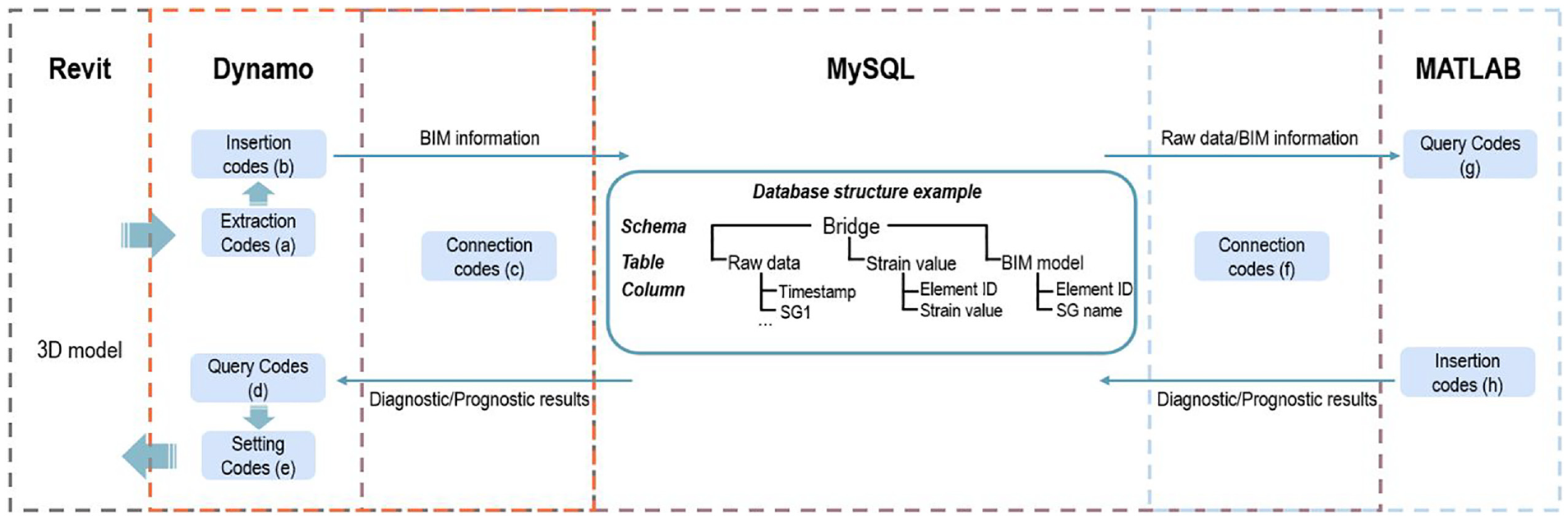
Figure 1 demonstrates the workflow of the proposed framework, which is composed of two parts: the data-driven SHM process and the BIM environment. In detail, the data-driven SHM process employs MATLAB as the analytical tool to perform diagnostic and prognostic evaluations, dedicated to extracting structural information relevant to bridge health. In parallel, the BIM environment leverages Revit-Dynamo as its foundational platform for the visualization of SHM data. Meanwhile, the MySQL database was adopted to store both the BIM model information and the SHM data due to its high compatibility with both the Revit-Dynamo environment and MATLAB, thus functioning as a crucial link between the BIM environment and the data-driven SHM process.
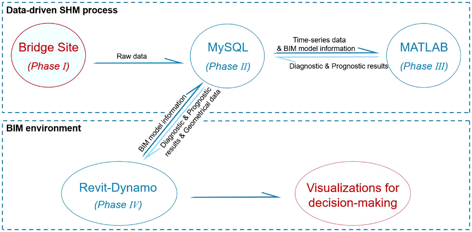
The workflow and data flow of the proposed framework.
The framework intends to provide automatic data flow among the four phases of SHM data. As shown in Figure 1, on-site collected raw data, including time-series data and geometrical data, is automatically transferred and stored in the MySQL database. 31 Sequentially, the geometrical data is queried using Dynamo for automatic model construction within Revit, 32 while the time-series data is queried and processed with MATLAB for diagnostic and prognostic evaluations. To actively involve the BIM model in the diagnostic and prognostic evaluations, associated model information is transferred to the analytical tool through the links built by the database. The outcomes of these evaluations are then synchronized with the BIM model information and re-routed into Revit-Dynamo for visualization. Consequently, diagnostic and prognostic insights are firmly connected and visualized with the BIM model.
Diagnostic and prognostic algorithms
Diagnostic algorithm
In this study, the algorithms developed for bridge diagnosis and prognosis are specifically tailored to the identification and visualization of critical areas on bridge deck, enhancing the clarity and accessibility of diagnostic and prognostic data. Strain data was selected for diagnostic analysis in this study due to its sensitivity to local structural damage and changes.33,34 The spatial distribution of strain across the bridge deck yields critical insights into both structural integrity and traffic dynamics, identifying the most deformed area on the deck and providing traffic patterns. To cost-effectively map the spatial strain distribution on the deck, the values collected by the SGs on-site are used to extrapolate the strains of adjacent areas according to specific rules detailed below.
It is assumed that when traffic load acts at the location of the SG, the strain distribution in the affected area of the load reaches its maximum at the location of the SG and decreases progressively with distance from the gauge following predefined strain mapping rules. The influence zone of each SG is defined as a circular area, centered at the location of the gauge. The strain value at a given location on the deck is determined as

where

where
On the other hand, by assuming a more gradual decrease in strain values from the center of the influence zone and consequently, more conservative results, a normal distribution rule is also considered to calculate the corresponding SCC
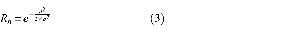
Similarly, the standard deviation
Prognostic algorithm
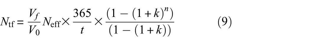
In this study, the prediction of residual fatigue life is performed in two steps using field strain measurements, employing the classical approach35,36 of combining the S − N curve with the cumulative damage law. 37 A schematic flowchart of the fatigue analysis is presented in Figure 2. In detail, residual fatigue cycles are derived from the strain-time history through a sequence of processes, involving conversion to stress-time history, rain-flow counting, S − N curve analysis, and calculations based on Miner’s rule. 37 Subsequently, the obtained results are converted into residual fatigue years, utilizing an appropriate assumption that correlates fatigue cycle consumption with traffic volume growth.
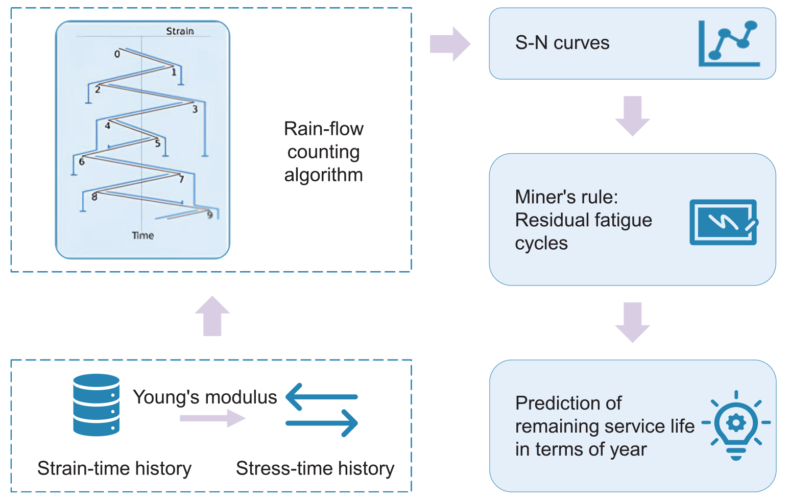
Schematic flowchart of residual life estimation.
In detail, on-site collected strain data is first converted to stress data by employing Young’s modulus relationship. 38 Following this conversion, the stress data is processed with the rain-flow counting algorithm, resulting in the generation of a stress-spectrum histogram. 39 Subsequently, the equivalent effective stress is calculated correspondingly as
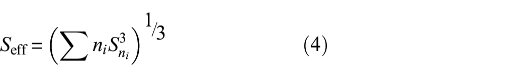
where
By employing Miner’s rule, which allows for the quantification of cumulative fatigue damage by correlating the stress cycles to their respective fatigue life contributions, the effective fatigue cycles that the bridge has sustained can be expressed as

where
For concrete bridge deck reinforced with steel rebars, which can be considered as a combination of several reinforced concrete beams,

In this case, each stress range
It is understood that vehicles with similar weight and speed running through the bridge would generate similar responses to the bridge. Consequently, after analyzing the data collected from the same SG with the rain-flow counting algorithm, the number of fatigue cycles consumed is expected to show minimal variation. On the assumption that the traffic component and the speed limit on the bridge are constant from its opening, the number of fatigue cycles consumed is therefore linearly related to the traffic volume. Given that the focus of this study is the bridges primarily subjected to traffic-induced damage, other factors that may contribute to the fatigue damage, such as the environmental effects, corrosion, and physical impacts, are neglected in this analysis. With these assumptions, this study modifies traditional life estimation methods, which typically generate fatigue cycles only, to the direct calculation of structural residual life in terms of year.
In detail, the linear relationship between the traffic volume and fatigue cycles consumed in the same year is assumed as
where
The total consumed number of cycles is the sum of the number of cycles consumed each year from construction to date, which can be illustrated as the sum of a geometric sequence by assuming a constant growth rate of traffic volume k per year as
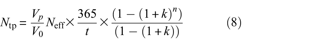
where
The residual number of cycles of the bridge,
where the only unknown variable is the number of residual years, n, which can be inversely calculated.
Data communication and visualization
To establish effective and precise connections between the Revit model and the diagnostic and prognostic analyses, and then achieve data visualizations within the BIM environment, it is crucial that the virtual model in Revit aligns with the physical structure in the real world. This alignment encompasses not only the primary bridge structures, such as the deck and piers but also the SHM system installed on the bridge. Sensors belonging to the SHM system should be accurately placed in the virtual model, mirroring their real-world layout. In accordance with the hierarchy-based paradigm employed by Revit,
41
the process of sensor modeling should proceed through a sequence of steps: selecting the appropriate category, creating a family, developing a type, and placing instances. Furthermore, it is essential to define instance parameters that reflect the functions of the sensors, thereby enabling the incorporation of data passed from the SHM system. Figure 3 presents an example of modeling SGs. A new family is created within the Data Devices category, incorporating a new type with a geometry of
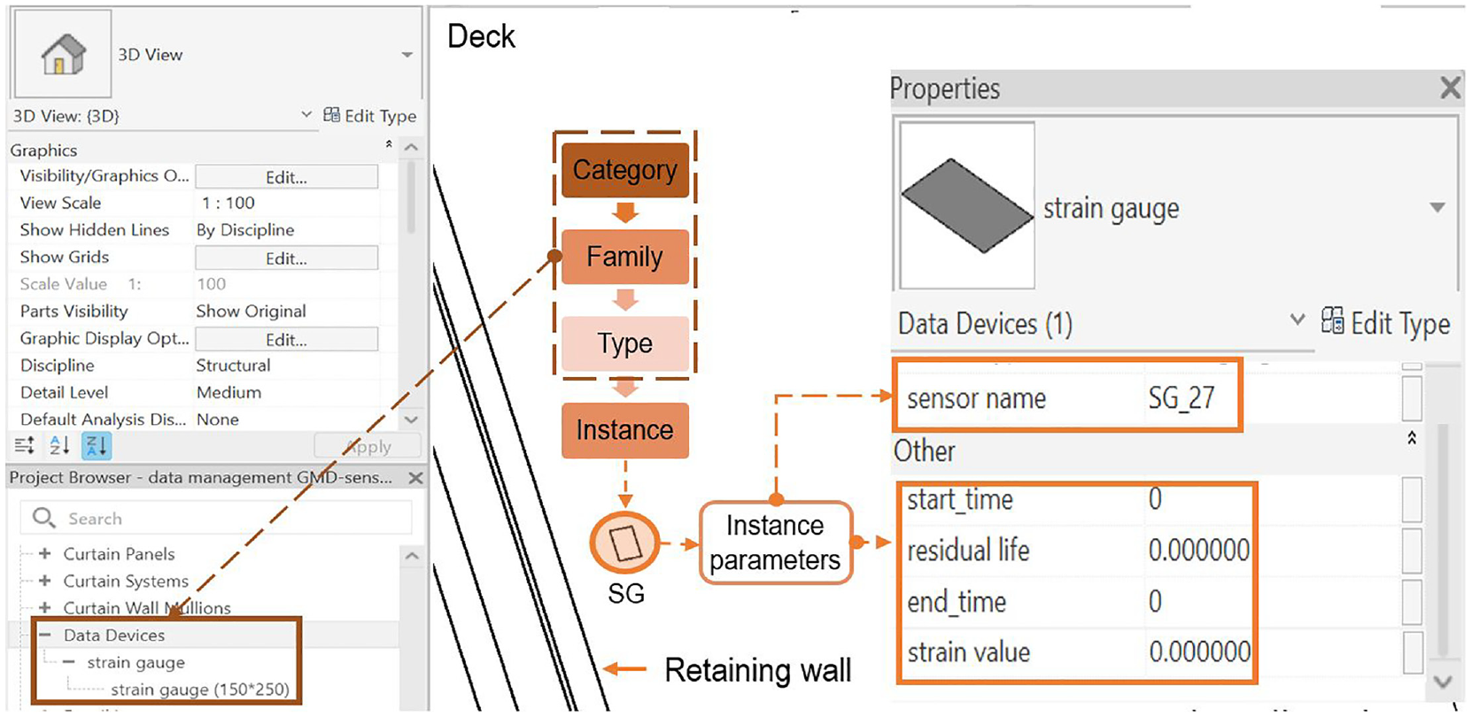
Hierarchy of the sensor family.
Based on the model alignments, data communication within the proposed framework is achieved through the established communication channels and a bidirectional mapping. Communication channels are established through Dynamo and MATLAB scripts, while MySQL database, gathering data from both MATLAB and Revit-Dynamo, is a crucial link for the mapping process. Raw data collected on-site is periodically transferred to the database, and the diagnostic and prognostic procedures are carried out on demand.
Figure 4 illustrates the detailed interactions between MATLAB, MySQL, and Revit-Dynamo in the proposed framework with an example of the database structure utilized. A schema (database) called Bridge is created with tables to hold data from different sources and for different purposes. For example, strain data collected on-site is periodically saved in table Raw data with timestamps as the primary key, and the strains from different SGs are stored in the corresponding columns. To pass the strain data to the BIM model, the element IDs and names of the virtual entities (VEs) of SGs are extracted and stored in table BIM model by adopting Extraction codes (a) and Insertion codes (b) as shown in Figure 5. The connection between the database and the BIM model is established with Connection codes (c) in Figure 5, while Query Codes (d) and Setting Codes (e) are adopted to query the evaluation results and update the corresponding parameters in the Revit model.
Data communication between MySQL, MATLAB, and the BIM model.
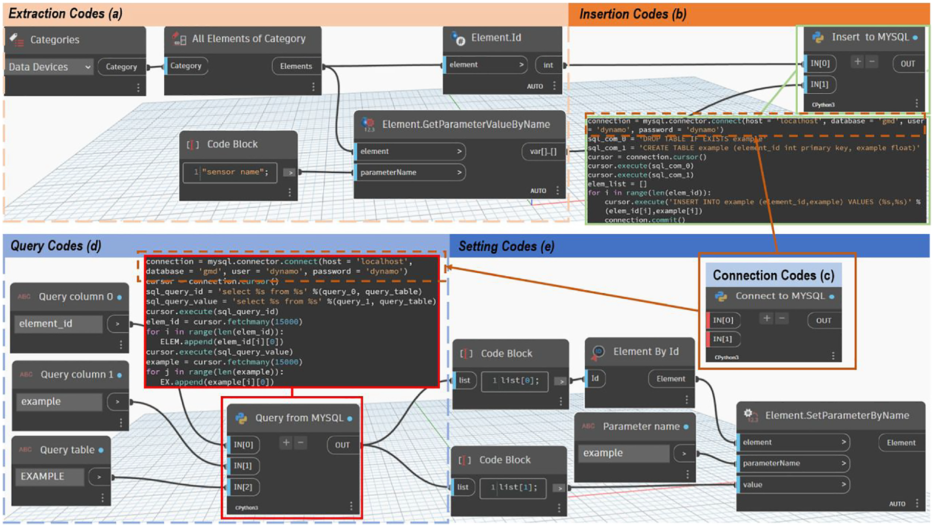
Examples of dynamo codes utilized for the communication between MySQL and the BIM model.
The database and MATLAB are connected using Connection codes (f) in Figure 6. MATLAB is configured with Open Database Connectivity (ODBC) drivers to ensure a robust and reliable connection. With the established tables Raw data and BIM model, the mapping process begins by querying both tables using Query Codes (g) in Figure 6, and the mapping results are returned to the Bridge schema as table Strain value through Insertion Codes (h). The mapping of the strain at a specific timestamp is detailed in Figure 7. Based on the consistency of the SG names, the strain values in table Raw data are aligned with the corresponding element IDs in table BIM model and inserted into the table Strain value. Dynamo then reads the Strain value table to update the Revit model, where the element IDs are read to locate the corresponding virtual SGs, and the strain value parameters of those VEs are populated with the corresponding strain values.
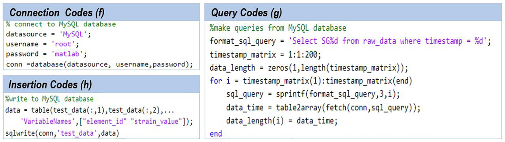
Examples of MATLAB codes utilized for the communication between MATLAB and MySQL.
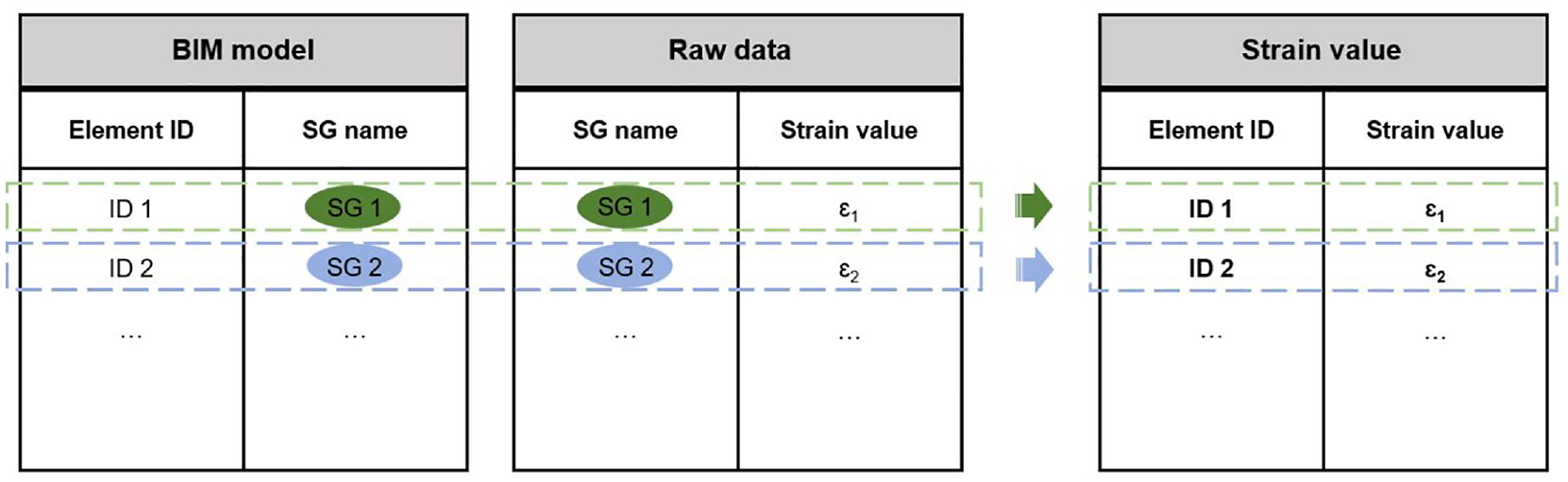
Strain data mapping example.
To facilitate the visualization of bridge local health, this study proposed to divide the monitored structure into finer partitions in the Revit model employing the Create Parts tab in the toolbar. Similar to the modeling of SGs, each partition is modeled with parameters to accommodate the required structural properties, allowing the visualization of structural properties in finer units. Specifically, to visualize the distribution of strains on the bridge deck, the distances between the virtual SGs and the finer partitions are calculated and then passed to the analytical tool, involved in the diagnostic analysis. Sequentially, the strains obtained are assigned to the finer partitions as parameters for visualization following the mapping process described. In this visualization scheme, varying colors are adopted to represent different strain intensities on the deck. Similarly, in the prognostic visualization, estimated residual fatigue years are mapped back to the BIM model as instance parameters of virtual SGs, with color variations indicating the likelihood of fatigue failure.
Case study
The Governor Macquarie Drive (GMD) bridge, situated in the suburb of New South Wales (NSW), Australia, is presented as a case study. Built approximately 30 years ago, this bridge consists of concrete culverts with two spans and three shear walls. In February 2018, the GMD bridge was extended as shown in Figure 8. Figure 8(a) provides a 3D view of the GMD bridge, including its detailed dimensions, while Figure 8(b) presents the top view of the GMD bridge with the installed SHM system and the extended part. To facilitate bridge health management, an SHM system consisting of 27 SGs and 18 accelerometers was installed to monitor the vibrational responses of this small-scale bridge.38,42 Figure 9(a) and (b) show examples of the sensors mounted on the bridge in real world. Additionally, the GMD bridge was thoroughly examined using a terrestrial laser scanner. Phase-based method was adopted and a FARO Focus scanner was utilized. Several anchor points were established using different reference locations to aid the creation of point cloud data. Over 10 h and 12 different locations were utilized for the scanning as shown in Figure 9(c) and (d).
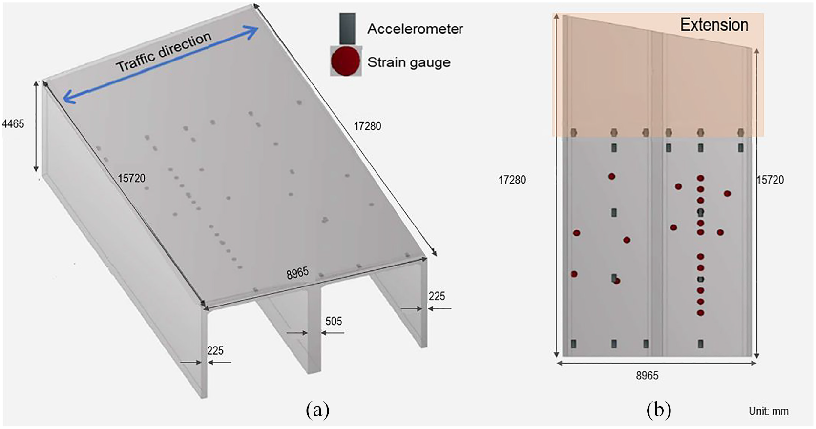
(a) 3D depiction of the GMD bridge and the installed SHM system (units: mm). (b) 2D top view of the GMD bridge and the installed SHM system.
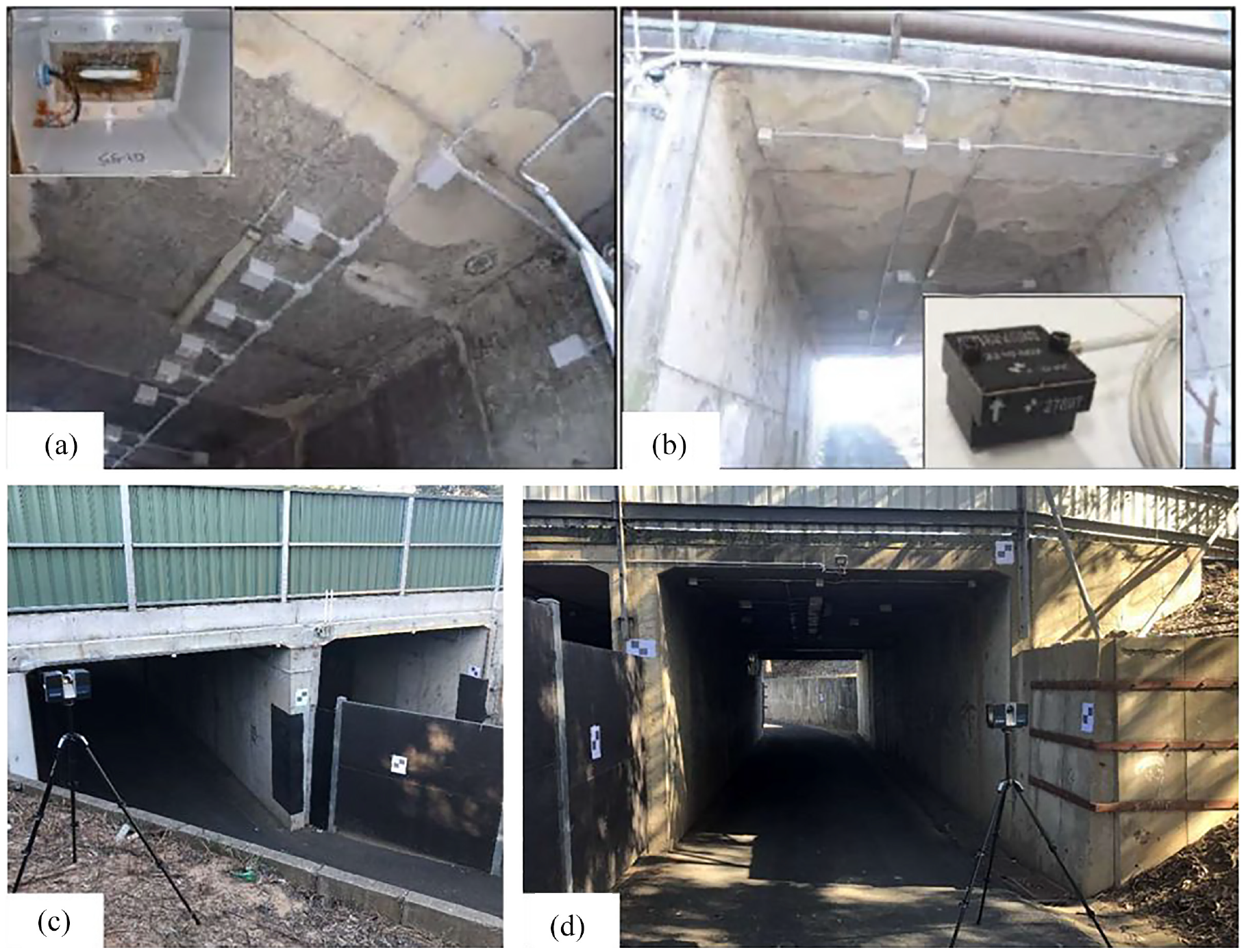
Photos for on-site data collections: (a) and (b) present sensor network on bridge deck, (c) and (d) show the device placement for point cloud data collection.
Model construction and alignment
The development of the BIM environment for the GMD bridge began with the creation of a 3D virtual model in Revit. To recreate the reality capture, the acquired 12-point cloud data files were integrated and combined using Autodesk Recap, as shown in Figure 10(a). It is essential to eliminate extraneous aspects from the reality capture, such as vegetation, unnecessary structures, automobiles, and obstructions. The results can be further simplified depending on the amount of information and point of interest as shown in Figure 10(b) and (c), where circles indicate different laser scanning positions. The resulting point cloud model was then transferred into CloudCompare for dimension measurement. The Revit 3D model was thus created with the measured dimensions.
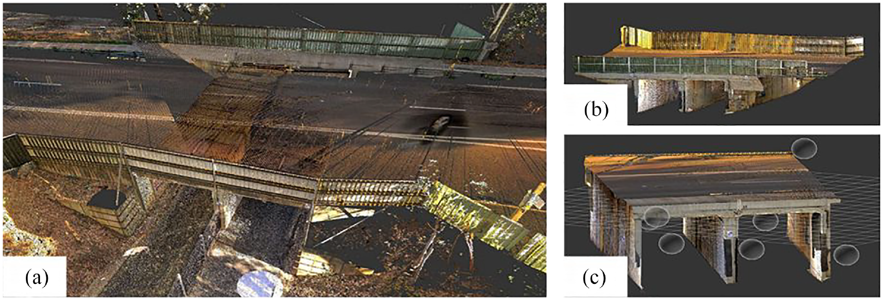
Process of constructing BIM model from point cloud data.
To streamline the analysis, this study focused exclusively on strain data, and therefore only the SGs from the installed SHM system were modeled. Parameters relevant to the diagnostic and prognostic analyses were established to facilitate data storage and subsequent visualization. In preparation for bidirectional data mapping, the element IDs of the virtual SGs were rigorously aligned with their respective names and recorded in the MySQL database. Figure 11 illustrates the Revit model of the GMD bridge, highlighting the setup for SHM data analysis and visualization.
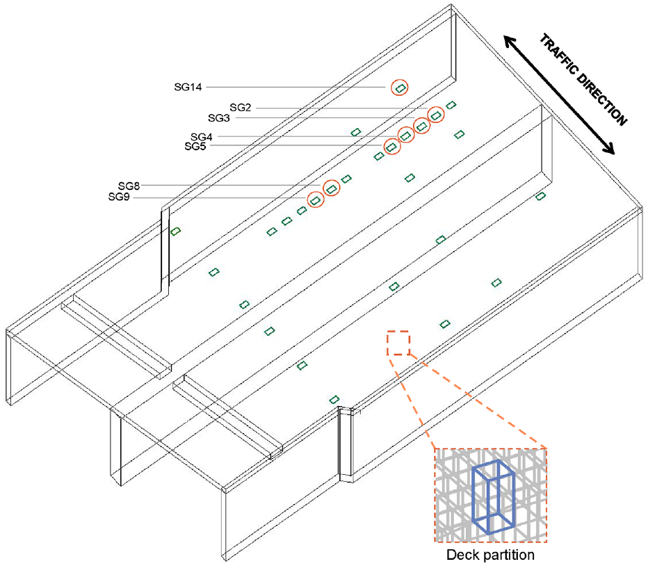
The 3D virtual model of the GMD bridge in Revit. Sensors circled have a residual fatigue life less than 60 years.
For the interactive diagnostic analysis in MATLAB, the bridge deck was partitioned into
The Dynamo scripts utilized for the distance calculation are presented in Figure 12. The coordinates of virtual sensor elements can be easily found in Dynamo with the help of standard nodes, such as Element.GetLocation. Since partitions belong to the bridge component that they are parted from and have no independent coordinates, Bounding Box nodes were adopted to locate the coordinates of the partitions. Bounding Box is the smallest possible orthogonal box that can fit the desired partitions inside. By calculating the geometrical center of such a box, the center of the corresponding partition can be identified. The distance data table, with a size of
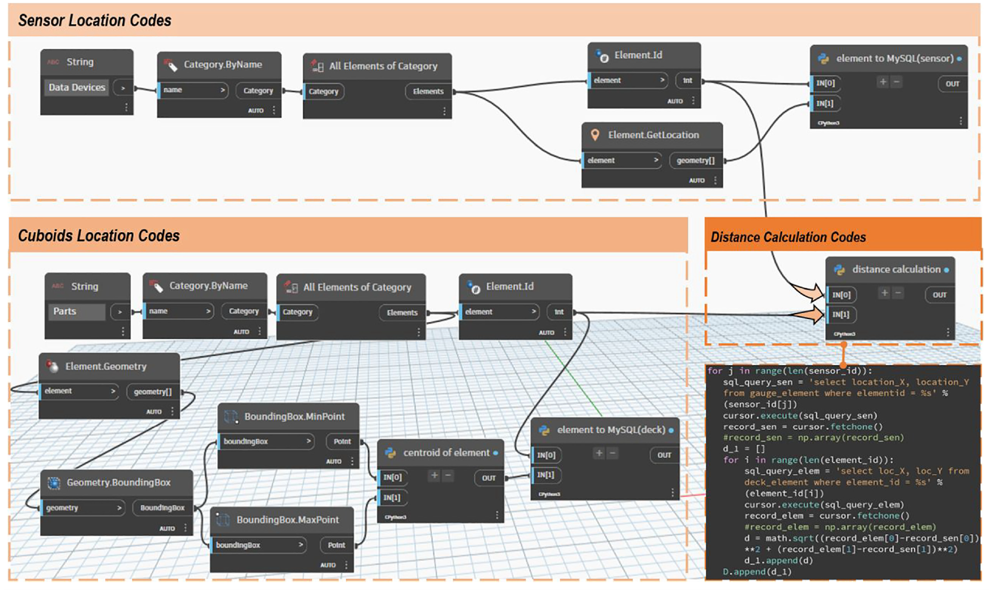
Examples of dynamo scripts for distance calculation.
Data-driven SHM process
Assuming that traffic follows the same pattern throughout the years, representative strain data collected on two independent sampling days with an interval of half a month were utilized for analysis. After denoizing, the strain data were compiled into two matrices for the subsequent diagnostic and prognostic analyses. These matrices, each with a size of
Diagnostic process
In order to cover most areas of the deck and avoid excessive overlapping, this study defined the diameter of the influence zone of each SG as 2 m. Thus, the parameters (
To enhance computational efficiency and reduce the workload, it was crucial to minimize the sizes of the SCC matrices. Only the non-zero elements in the SCC matrices were calculated and the strain of each cuboid at each sampling point of the SGs was calculated as

where
Prognostic process
In preparation for the application of the rain-flow counting algorithm, the strain-time data is first converted to the stress-time data (σ), followed by an essential pre-processing phase to eliminate the stress cycles that contributed insignificantly to the overall fatigue damage.
43
Figure 13(a) presents the processing of an 8-min strain data collected from SG 8 to locate the maximum and minimum values of each stress cycle. While these values were retained, the intermediate data points were removed as shown in Figure 13(b). The rain-flow counting algorithm was then applied to the stress data, and the resulting stress-spectrum histogram presented in Figure 13(c) was adopted for the calculation of effective cycles (
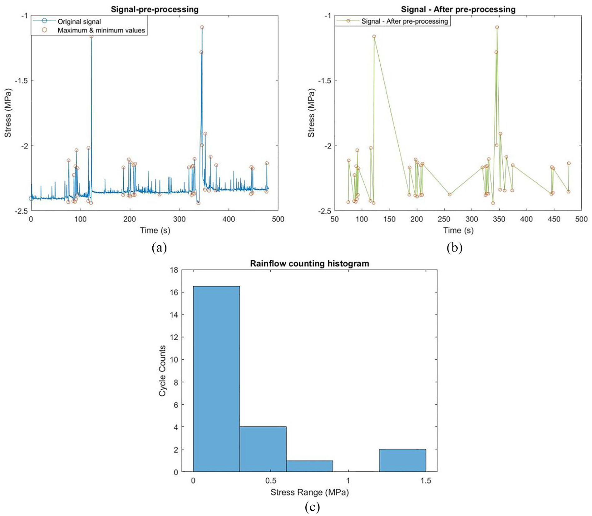
Example of strain data processing: (a) Example of data processing with original data, (b) Example of data processing with stress data that contributes to fatigue cycles, and (c) Stress spectrum histogram.
To accurately calculate the residual fatigue life of the bridge in terms of years, it is essential to first determine the unknown variables in Equations (8) and (9). These variables include the traffic volume at the time when the bridge was constructed (then traffic volume) and the current traffic volume, as well as the sampling time of the SGs. For this case study, the then traffic volume

In this study, the strain data was collected over two distinct days, thereby establishing the sampling time for the SGs as 1 day. Consequently, the variable
Based on the variables identified, the total consumed cycles (
Residual fatigue years less than 60 years.
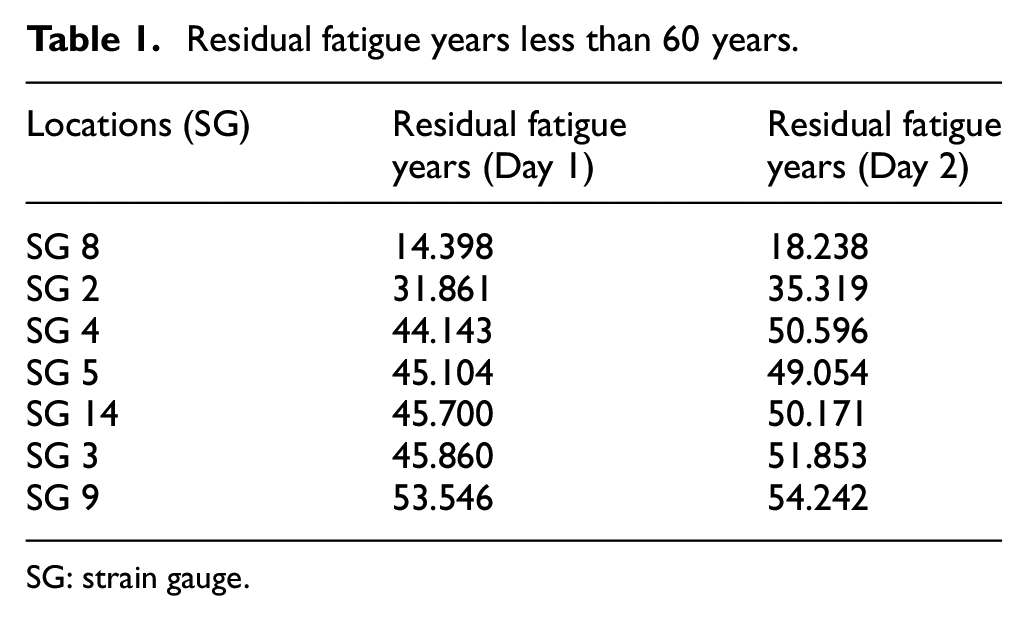
SG: strain gauge.
Diagnostic and prognostic visualizations
With the preparations above, the visualizations of diagnostic and prognostic results were achieved along with the 3D virtual model of the GMD Bridge in Revit as shown in Figure 14(a) and (b). The strain values and residual fatigue life were mapped to their corresponding parameters of the partitions and virtual SG entities, respectively. Then, color-coded schemes were employed to represent varying levels of strain intensity and residual fatigue life duration. Additionally, as shown in Figure 14(c), real-time sensor data were visualized with the virtual 3D model as raster images, each linked to the corresponding parameters of the virtual SGs. The use of Dynamo for the real-time sensor data visualization provided detailed insights into the strain data, further enriching the understanding of the structural health of the bridge.
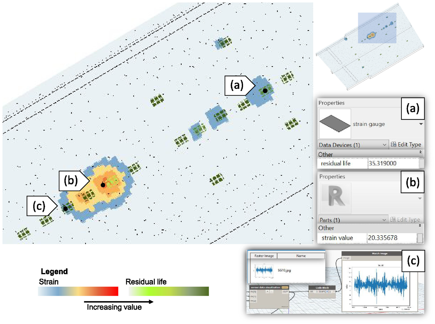
Visualization of structural information in Revit: (a) Prognostic data visualization (Residual fatigue life), (b) Diagnostic data visualization (The most deformed area), and (c) Real-time sensor data visualization.
The visualizations of the daily maximum strain the bridge experienced are presented in Figure 15, while Figure 16 shows the distribution of the daily average strains. In both figures 15 and 16, Figure (a) and (c) depict the strain distribution derived from the strain data collected on Day 1, while Figure (b) and (d) illustrate the results from Day 2. The strain distributions in Figure (a) and (b) are based on the normal distribution rule, whereas Figure (c) and (d) are the outcomes of the negative linear relationship rule. Each figure features a zoomed-in view of the critical area, located in the left corner. Figure 15 provides the information for timely identification of anomalies, while Figure 16 presents a long-term pattern of the strains along the deck.
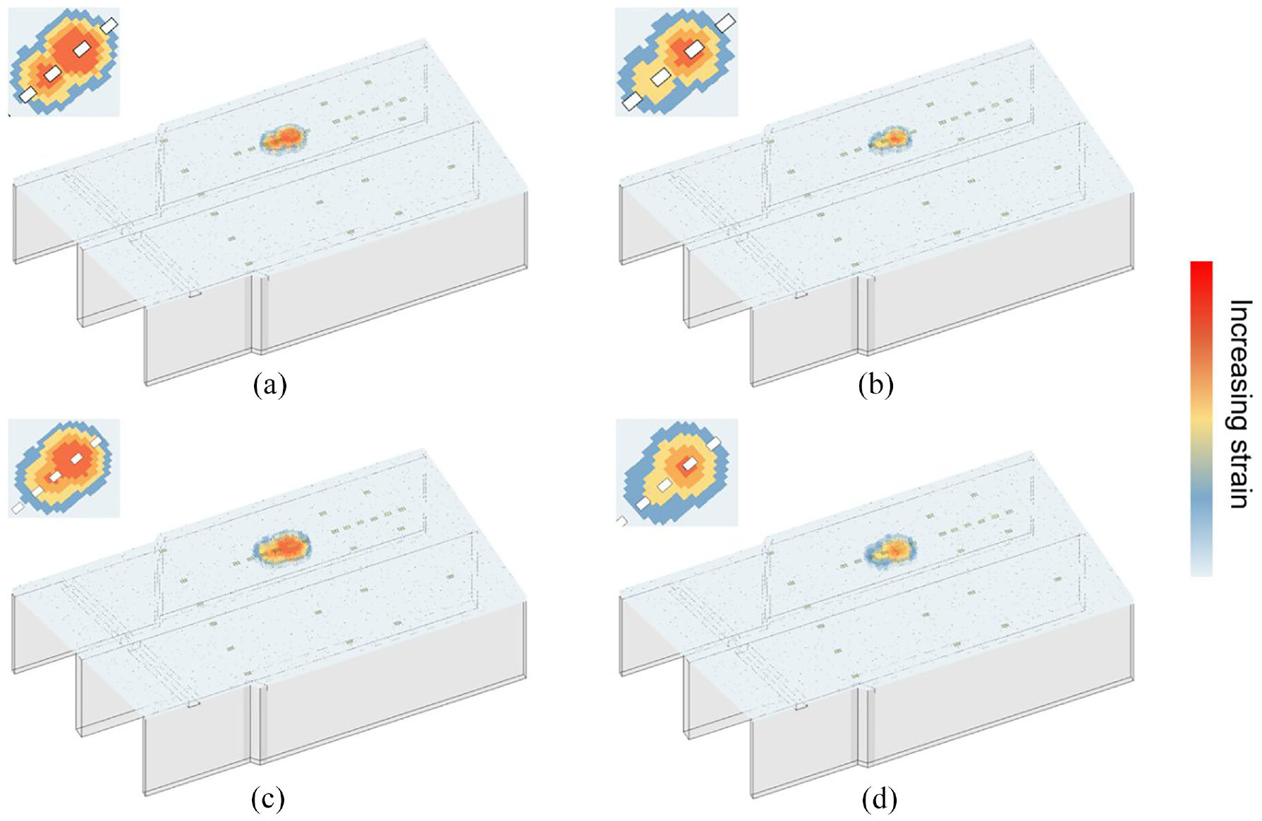
Maximum strain distribution on the deck. (a) and (c) Strain distribution of Day 1 under normal distribution and negative linear relationship rules, respectively. (b) and (d) Strain distribution of Day 2 under normal distribution and negative linear relationship rules, respectively.
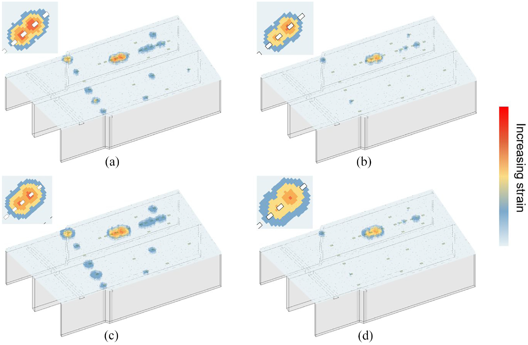
Average strain distribution on the deck. (a) and (c) Strain distribution of Day 1 under normal distribution and negative linear relationship rules, respectively. (b) and (d) Strain distribution of Day 2 under normal distribution and negative linear relationship rules, respectively.
It was also observed that larger areas were highlighted in orange under the normal distribution rule, which seems particularly sensitive to large loadings and tends to yield more conservative results. In contrast, the negative linear relationship rule distributes the recorded strains over a broader range, offering a different perspective on the strain distribution. Notably, in all figures, the area near SG 8 is highlighted in orange, indicating the highest strain intensity on the deck and identifying it as the most critical area, which is consistent with the prognostic results in Table 1.
The visualization details of the prognostic results are depicted in Figure 17(a) and (b) based on the data collected on Day 1 and Day 2, respectively. In this scheme, deeper shades of green correspond to longer residual life spans. In both Figure 17(a) and (b), SG 8 is distinctly highlighted in light green, signifying the location with the shortest calculated residual life spans, and therefore is the most critical location on the deck. It is important to note that the predicted residual fatigue life does not necessarily indicate an imminent structural collapse at the end of the estimated period. Rather, it serves as a valuable indicator for determining the timing of critical maintenance and the frequency of necessary on-site inspections.
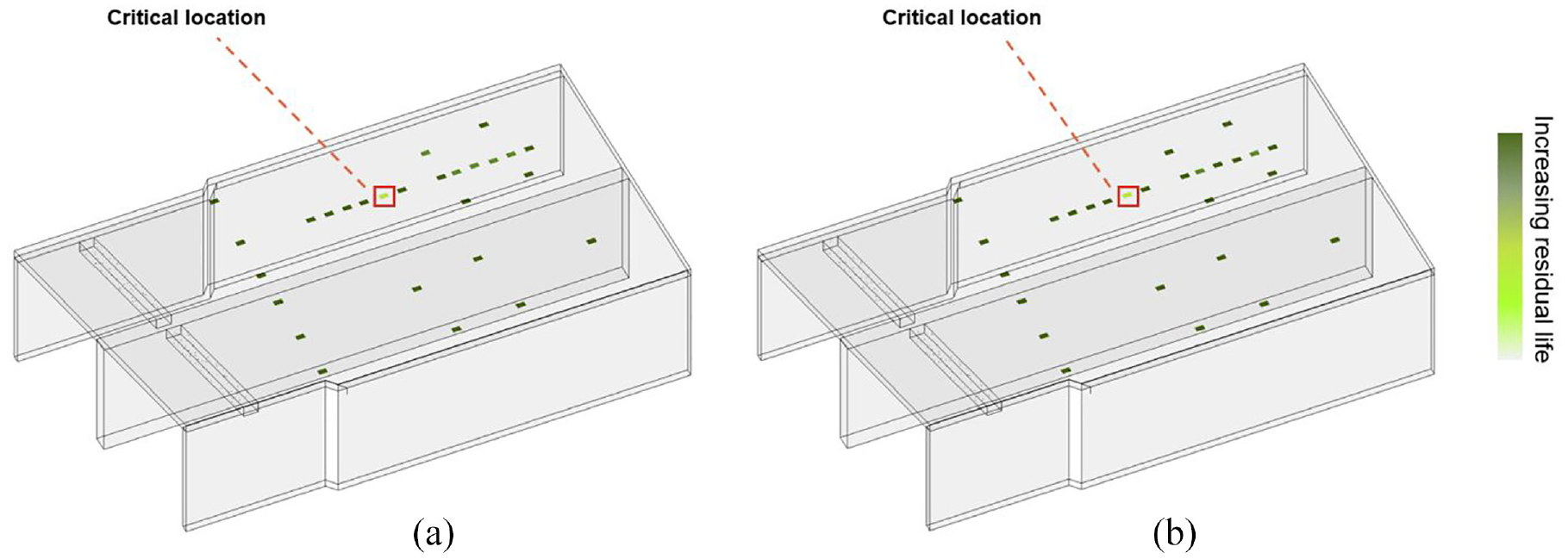
Visualizations of prognostic results: (a) and (b) Showing the results obtain from Day 1 and 2, respectively.
Discussion
This study aimed at aiding bridge O&M phases monitoring through the integration of BIM techniques and data-driven SHM. The proposed methodologies were effectively demonstrated through a two-span reinforced concrete bridge as a case study. Though data analysis and 3D visualizations for diagnosis and prognosis were achieved with on-site collected strain data, limitations and challenges for the current framework still exist.
Firstly, the proposed framework adopted a relational database, which has inherent drawbacks when dealing with large datasets although it is highly compatible with both Revit environment and MATLAB. Moreover, it is also limited in processing unstructured or semi-structured data, which is common in bridge health monitoring.
Secondly, since the proposed framework was ad hoc designed for SHM data visualization and bridge local health monitoring, the diagnostic and prognostic algorithms rely heavily on field strain measurements, which may limit their applications to road bridges that are mainly subjected to cyclic traffic loading only. The generality of the effectiveness of the proposed framework for other types of bridges with different loading conditions will be the focus of future studies.
Thirdly, though the update of structural behavior such as residual fatigue life is achievable by adopting the proposed framework with new data collected by on-site sensors, challenge still exists in ensuring the dynamic updating and management of the BIM model throughout the entire lifecycle of the structure. To support the full-life monitoring of bridges and ensure the BIM model to be an accurate tool for long-term structural management, it is indispensable to dynamically integrate more critical information such as bridge damage and subsequent repairs or interventions into the BIM model over time.
Conclusion
This study introduced a framework that utilizes the BIM techniques for bridge SHM, supporting bridge diagnostic and prognostic analyses while facilitating their visualization. To achieve this, the data communication channel between the data-driven SHM process and the BIM environment was established, allowing bidirectional data mapping. Additionally, the study has proposed and customized diagnostic and prognostic algorithms specifically designed for graphical presentation within the BIM environment, thereby enabling intuitive visual assessments of bridge integrity and longevity.
The proposed algorithms were applied to a case study bridge. The BIM model was actively involved in the diagnostic and prognostic evaluations by embedding the geometrical information of the virtual model into the evaluation processes. The 3D visualization of diagnostic and prognostic data directly related the potential damage with the dimensions of the structure, improving the precision for damage localization. The visualization of diagnostic data is capable of being updated within seconds, accurately reflecting the distribution of strains across the entire deck for each sampling point of the SGs. The graphical presentation and visualization of the diagnostic and prognostic data provided timely identification of structural issues and traffic patterns and assisted in the long-term planning of maintenance schedules.
Footnotes
Declaration of conflicting interests
The author(s) declared no potential conflicts of interest with respect to the research, authorship, and/or publication of this article.
Funding
The author(s) received no financial support for the research, authorship, and/or publication of this article.