
Abstract
Induction motors (IMs) play a pivotal role in various industrial applications, powering critical systems such as pumps, compressors, fans, blowers, and refrigeration and air conditioning systems. Monitoring the health of these IMs is essential for ensuring reliable operation. Numerous sensors, including vibration, current, temperature, acoustic, and power sensors, can be employed for their health monitoring. This article conducts a comprehensive comparative analysis of two widely used sensors—vibration and current, for classifying different health states of IMs, such as a healthy condition, bearing fault, and misalignment. The study employed deep learning techniques, specifically 1D and 2D convolutional neural networks, trained on raw data. Additionally, machine learning techniques, including random forest and XGBoost, were utilized and trained on features derived from preprocessed signals using fast Fourier transform and discrete wavelet decomposition. Comparative results indicated that vibration signals achieved remarkably high accuracy, nearly 100%, in detecting the investigated mechanical faults, while current signals, after signal processing and manual feature extraction, achieved an accuracy of 87.41%. These results demonstrate that, though current sensors are a viable alternative to vibration sensors, their performance can be affected by the type and degree of the considered faults. This study also highlights the attributes of vibration and current signals in the health monitoring of rotating machinery such as IMs.
Introduction
Induction motors (IMs) are used in diverse industrial applications, and they make up nearly 85% of all the motors used in manufacturing equipment and operations. Their low cost, robust structure, and reliability make them suitable for many applications such as conveyors, cranes, compressors, and pumps.1,2 Nonetheless, the harsh operating conditions IMs are subjected to, which include overload and sudden load change, cause the mechanical and electrical parts to experience faults.3,4 Such faults include bearing faults, misalignment, eccentricity, stator winding faults, rotor bar faults, etc. 2 Hence, it is important to develop a fault diagnosis system for IMs to prevent unplanned downtime and reduce maintenance costs by optimizing the process.
The three methods of diagnosing IM faults are model-based, signal-based, and artificial intelligence (AI) methods. 5 The first two methods, model-based and signal-based, are traditional methods and they require high-level domain - expertise to implement. In the model-based method, the governing equations or mathematical model describing the behavior of a system are used in diagnosing fault conditions, while the latter method uses signal-processing techniques to detect patterns that are distinct to each fault case. 6 These two methods not only require expert knowledge; they also take an ample amount of time and may lead to inaccurate results in diverse industrial scenarios.
The recent or modern method, which is intelligent fault diagnosis, leverages system data and machine learning (ML) or deep learning (DL) algorithms such as random forest (RF), K-nearest neighbor (KNN), support vector machine (SVM), artificial neural network (ANN), and convolutional neural network (CNN), and its results in the fault diagnosis of IMs are very promising.5,7 Performing intelligent fault diagnosis often involves extracting features from preprocessed signals using techniques such as fast Fourier transform (FFT) and wavelet transform (WT). This enables the extraction of relevant information from raw signals for effective analysis. Among the DL models, CNNs have recently become increasingly popular because of their effectiveness in extracting features directly from raw data, without the need for manual feature extraction, which takes time when multivariable signals are used.5,8 In other words, DL methods circumvent the time it takes to perform signal processing, which can be significant when dealing with datasets with large data points and channels.
Furthermore, the signals used in the condition monitoring of IMs include current, vibration, acoustic, thermal, etc. However, to rank the usage of different signals in literature, vibration comes first, followed by current signals. Vibration signals are very sensitive to mechanical faults and are well-researched. However, vibration signals are expensive because external sensors like accelerometers are needed to be installed on the IM.3,9 Current signals are cheap to acquire from the test rig current transformers or through the use of a current transducer. Besides, current signals are considered nonintrusive for condition monitoring because the measurement is typically carried out without physically coming in contact with interfering with the IM being monitored. The downside to current signals is that they are sensitive to electrical characteristics. 10 Therefore, the objective of this research is to investigate the effectiveness of using current signals from IMs in diagnosing weak mechanical faults.
The contribution of this article is summarized in two points. First, the performance of vibration and current signals are investigated in the classification of an induction motor state, under two mechanical fault scenarios (misalignment and outer bearing fault). Second, the article conducts a rigorous comparative analysis, evaluating the efficacy of widely used ML and DL methods in this context, thereby providing valuable insights into the most effective approaches for fault diagnosis in induction motors (IMs).
The remaining parts of this article are structured in the following order: a comprehensive literature survey that explores the utilization of different signals and both ML and DL algorithms for condition monitoring. The subsequent sections detail the experimental methodology, encompassing the setup for data acquisition and the application of DL models. Conversely, the use of ML models is covered, including various types of feature extraction techniques and the application of different ML models. The article follows by presenting the results, conducting a comparative analysis, and engaging in a thorough discussion. The concluding remarks encapsulate the key findings and implications drawn from the study.
Brief review of condition monitoring of IMs
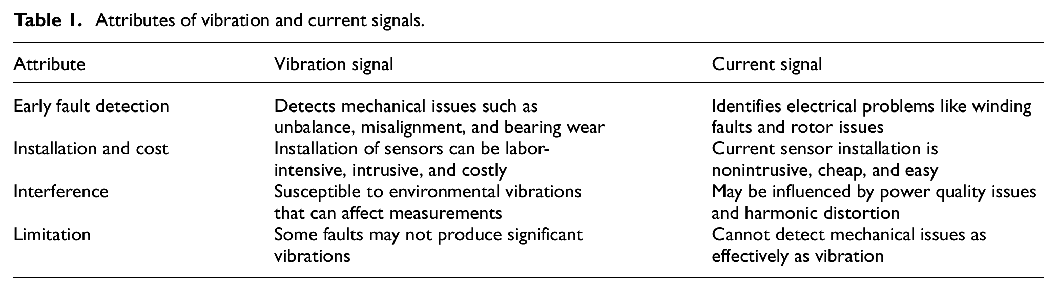
The two main signals used in the condition monitoring of an induction motor are vibration and current. The choice of any of these signals depends on the operating conditions of the motor and the examined fault. For instance, condition monitoring using vibration signals can pose challenges, primarily because of the impact of background noise and variations in the rotational speed of components. Additionally, during the initial phases of a defect, the signal containing pertinent information about the anomaly may become obscured by concurrent vibration phenomenon. 11 While vibration monitoring yields exceptional results in detecting mechanical faults such as bearing issues, imbalance, or misalignment in small-rated IMs, its accuracy diminishes when applied to high-rated induction machines. On the other hand, during operation under low-load conditions, the current signal might lack adequate information to differentiate specific mechanical faults. However, the subsequent impact of these mechanical issues, such as rotor or bearing faults, can manifest in the failure of electrical components like high-resistance contacts within IMs, causing abrupt variations in the current signal. This phenomenon enhances the effectiveness of current signature analysis. 12 To summarize, the important attributes of vibration and current signals are discussed in Table 1.
Attributes of vibration and current signals.
In recent years, with the evolution of advanced intelligent algorithms and fast computers, significant progress has been made in the field of health monitoring of IMs. Many research works have been conducted on the intelligent fault diagnosis of an induction motor using knowledge-based methods and signal processing methods. Figure 1 shows an overview of intelligent fault diagnosis using AI techniques. Diagnostic methodologies in the context of condition monitoring can be broadly classified into two categories: feature-based and raw time series data-based approaches. Feature-based techniques typically follow a two-step process, involving meaningful feature extraction as the first step and subsequent decision-making as the second. These features may span various domains, including time, spatial, frequency, or time–frequency. Additionally, combinations of features derived from different domains are often employed to enhance the diagnostic accuracy and robustness of the methodology.
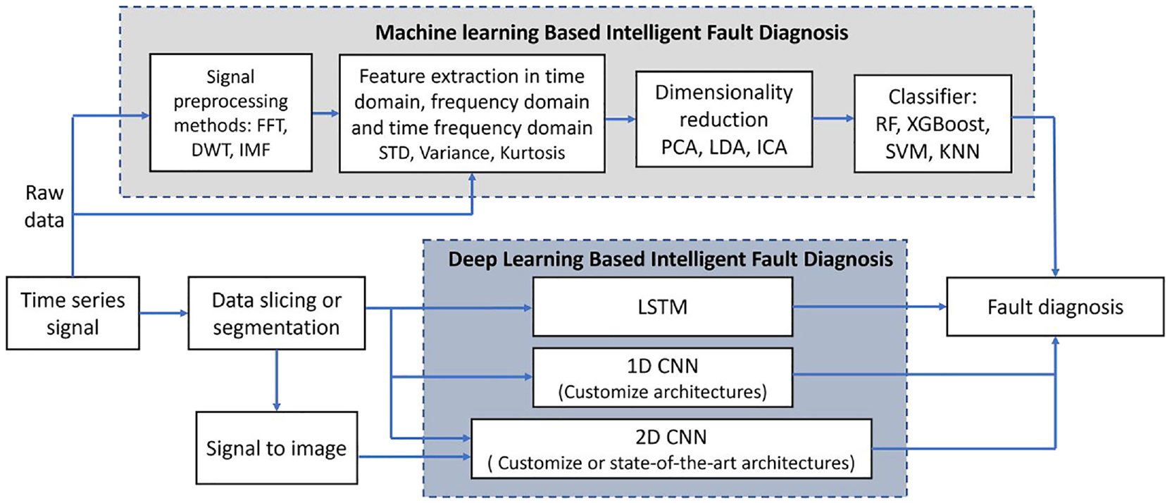
Intelligent fault diagnosis using AI techniques.
In the domain of AI-driven methods, ML techniques have been extensively employed for fault detection and diagnostics. However, addressing the limitations inherent in ML, such as the challenge of learning directly from raw data and the reliance on domain experts for feature extraction and selection, DL methods have gained prominence, enhancing both the reliability and efficiency of fault diagnosis. 13 DL employs neural networks (NNs) with extended chains of layers to learn hierarchical features from input data. Various DL architectures, including CNNs, recurrent neural networks, and long short-term memory, have been developed to improve machine health monitoring performance using extensive datasets collected from multiple sensors. CNN, recognized as a state-of-the-art DL approach, particularly stands out for fault diagnosis due to its capability to transform intricate information into multilevel classification tasks. A standard CNN architecture is characterized by a sequential arrangement of convolutional layers and pooling layers, often stacked alternately. This summary will focus on CNN-based induction motor fault diagnosis within the broader context of DL methods.
DL on vibration and current signal
For example, Sun et al. 14 used 1D CNN with convolutional discriminative feature learning to extract features from raw vibration signals and classify the health states using SVM. The combined CNN and SVM approach achieved an accuracy of 97.8% in classifying six health states, surpassing supervised CNN by 14%. Hoang and Kang 15 used 2D CNN for bearing faults diagnosis using vibration signals, and the model was trained on the Case Western Reserve University/CWRU dataset. 16 An architecture comprising two convolution layers with each followed by a subsampling layer was proposed. The obtained classification accuracy was 100%. The performance of 2D CNN, 1D CNN, and SAE were compared. When the signal-to-noise ratio (SNR) was −10 dB, 2D CNN gave 97.74% accuracy while 1D CNN gave 90.75% accuracy. A similar work with the same dataset was reported by Zhang et al., 17 where a 2D CNN architecture with two convolution, two pooling, and two fully connected layers was proposed. The results showed that the proposed method outperforms the other methods (i.e., raw 1D + 1D CNN and FFT + ANN). Also using vibration signals, two datasets (CWRU and Intelligent Maintenance System/IMS datasets 18 ) were used to train a 1D CNN. 6 The 1D CNN classifier gave an accuracy of 93.9% for IMS and 93.2% for CWRU-bearing fault classification.
In contrast, there exist studies highlighting the viability of utilizing current signals for the health monitoring of IMs. One such initial investigation by Schoen et al. 19 explored the effectiveness of current monitoring for detecting bearing faults. The study correlated the relationship between stator current and vibration signals, capitalizing on the understanding that bearing faults induce variations in air gap flux density, consequently altering the current spectrum. The findings concluded that, with adequate spectral resolution, the harmonics present in the stator current spectrum serve as reliable indicators of rolling-element bearing faults. Building upon these findings, the researchers further developed their work to detect motor faults. They employed an unsupervised method that involved transforming the time series current signal into a frequency-domain spectrum. Subsequently, a rule-based frequency filter was applied to select dominant harmonics, and a neural network was employed to identify any changes in the spectrum compared to that of a healthy motor. 20 However, it is noteworthy that this rule-based filtering approach necessitated expert knowledge, and the method exhibited limitations in its ability to classify between various types of faults. Motor current signal was used to train a 1D CNN for bearing faults analysis by Ince et al. 21 The proposed model has three convolutional layers followed by two fully connected layers. The result shows 97.4% accuracy. The structure of 1D CNN is simple, and it is easier to deploy to hardware. Current signal was also used by Gundewar et al. 22 but the states considered are healthy, and four broken bars faults of different severity. Different CNN architectures were trained based on the input image pixel sizes, learning rate, and minimum batch size to identify the best 2D CNN architecture. The average classification accuracy of the CNN models is 99.58%.
In the work of Samuel et al., 23 multisensory signals, including vibration, current, voltage, and speed, were gathered from an induction motor test stand across various operational scenarios: healthy operation, shaft misalignment, and outer bearing fault. These signals were used in seven different combinations to train 1D and 2D CNN architectures for motor fault classification. A comparative analysis was conducted to evaluate the diagnostic accuracy, parameter count, and computational time of the CNN models. Results revealed that utilizing only the motor’s vibration signals for training both 1D and 2D CNN models yielded optimal performance. Additionally, the 2D CNN model demonstrated slightly superior validation accuracy compared to the 1D CNN across different multisensory signal combinations. Motor current from multiple phases of current was used by Hoang and Kang, 24 and feature sets were derived through the application of CNN to the current signal of each phase. An information fusion technique at the decision level was employed to combine the information extracted from all the individual CNNs. The utilization of this merged information yielded a notably elevated fault detection accuracy of 98.3%, surpassing the accuracy achieved with a single current phase, which stood at approximately 91%. It is noteworthy, however, that the accuracy obtained through this approach using vibration signals was even higher at 99.47%. Nonetheless, employing a conventional CNN for fault detection based on raw signals proves to be computationally expensive, constraining its applicability in real-time scenarios. To address this limitation, an accelerated CNN was specifically designed for detecting bearing faults in IMs. 25 While the proposed method demonstrated a slightly higher accuracy compared to the classical CNN, its advantage lies in computational efficiency, being three times faster in terms of processing speed.
To enhance fault classification accuracy and ensure model stability using a single sensor, multiple sensor signals—both vibration and current—were concurrently employed with their time–frequency images (i.e., WT) serving as inputs to the deep architecture. The multisignal model, featuring three 2D convolutional layers, achieved an accuracy of 99.83%, surpassing the individual accuracies obtained with only vibration (98.72%) or current (98.26%) signals. 26 Other CNN variants, such as temporal convolutional networks (TCNs) 27 and attention mechanism enhanced TCN, 28 along with pre-trained models like RESNET-50, 29 have also been explored in the literature.
ML on vibration and current signal
Utilizing ML algorithms for health monitoring of IMs involves preprocessing raw data to extract feature matrices, serving as inputs to classifiers. Various statistical models such as mean, median, kurtosis, skewness, standard deviation,30,31 and frequency and time–frequency domain analyses such as FFT, 32 short-time Fourier transform (STFT), 33 wavelets, 3 Hilbert-Huang transform, 34 and sparse decomposition 35 have been employed in literature for feature extraction. Meanwhile, powerful ML models, including SVM,31,36,37 KNN,31,37,38 ANN, 39 Decision Trees, 40 Random Forests, 36 and Naïve Bayes classifiers,36,37 find widespread application in this context.
SVM integrated with the binary particle swarm optimization algorithm for feature selection, aimed at maximizing class separability, was employed in the detection of bearing faults by Ziani et al. 41 The approach achieved 100% accuracy with an optimal feature set tailored for various fault conditions, including inner race, outer race, and rolling element faults. Nishat and Kim 3 used discrete wavelet transform (DWT) and ML to develop a fault diagnostic model for inner and outer bearing faults with current signals. Three different mother wavelets (db4, sym4, and Haar) were examined in the DWT of the current signals obtained from an induction motor. A notch filter was used at the preprocessing stage to remove the current signal supply frequency, which is 60 Hz, and two ensemble ML classifiers (RF and XGBoost) were trained based on 11 time–frequency domain features extracted from DWT coefficients at the 11th level. An accuracy of 99% was obtained using the filtered signal with all three-mother wavelets and the two classifiers. No feature selection was done. DWT and ANN were used by Zuhaib et al. 42 to diagnose rotor bars and high contact resistance faults. The mean and RMS features were extracted from the resulting wavelets of current signals gotten through DWT and an ANN model was trained for fault classification. The results revealed the mean features yielded a classification accuracy of 98%, which is better than RMS features.
Gaps in the existing literature
The comprehensive literature survey reveals that both vibration and current signals offer valuable insights into the health of IMs. However, these signals inherently convey distinct information, serving as useful indicators for different fault conditions. While certain ML or DL models exhibit efficacy with vibration data, others excel with current signals. Previous studies have focused on either ML or DL models exclusively, leaving a notable gap in the literature regarding a comprehensive comparison among popular ML and DL models when applied to both vibration and current signals. Addressing this gap, this article seeks to present an in-depth analysis and comparison of these models, bridging the knowledge divide and contributing to a more holistic understanding of induction motor health monitoring.
Research questions and objectives of this study
Based on the identified research gap, the research questions that serve as the driving motivation for this study are:
Can current signals, which are nonintrusive and typically associated with electrical faults, be effectively used to replace vibration signals in the classification of motor mechanical faults?
Can DL models perform accurately without relying on feature extraction when diagnosing fault-weak signals?
When adapting the feature-based method, which type of feature (in frequency and time–frequency domains) will be more effective in improving the accuracy of fault classification?
To address these research questions, the following objectives have been established:
Compare the effectiveness of current and vibration signals in the diagnosis of common motor mechanical faults.
Evaluate the performance of two popular DL models (1D and 2D CNN) without performing explicit feature extraction.
Investigate the extraction of fault features from preprocessed current signals through FFT and DWT and observe their impact on the accuracy of ML classifiers (RF and XGBoost).
In contrast to majority of studies that rely on vibration signals for fault diagnosis, this research focuses on enhancing the accuracy of current signature analysis in detecting weak mechanical faults through signal preprocessing. By combining frequency domain (FFT) and time–frequency domain (DWT) features, this study offers a promising alternative to traditional methods that predominantly depend on vibration-based diagnostics.
Methodology
This methodology section encompasses the experimental setup for data acquisition and the DL models examined in this work are presented. In addition, the ML models used are discussed along with various types of feature extraction techniques used with them.
Experimental setup
The Centre for Efficiency and Performance Engineering, University of Huddersfield (UK), induction motor experimental test rig was used for a series of experiments that produced the dataset used in this article. An AC induction motor, a DC loading generator (4 KW, 1500 rpm), flexible coupling, and a few sensors make up the test rig in Figure 2. The induction motor was designed with a rated speed of 1730 rpm, operated at a frequency of 50 Hz, and had a rated power of 4.5 kW (5.5 HP). Two accelerometers, one on the vertical side and the other on the horizontal side of the induction motor, were installed to acquire vibration signals, while the three-phase current signals were measured from the current transformer (in the control box).
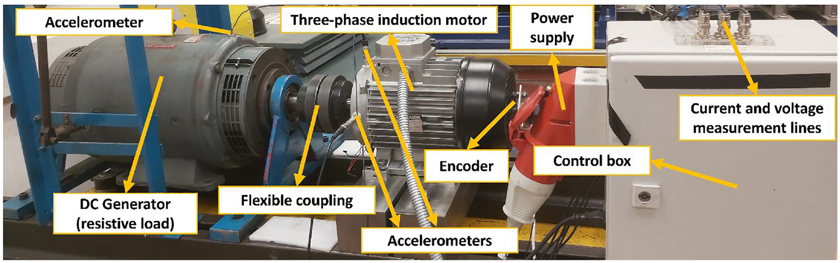
Induction motor test rig. 23
In addition, three separate situations/states, that is, healthy condition, misalignment, and outer bearing fault, were considered. A series of 15 experiments were carried out for each of these situations according to the design shown in Table 2, which demonstrates the variance in test load and speed under various test scenarios. The load settings (0%, 20%, 40%, 60%, and 80%) represent different levels of mechanical stress, from no load to near full load while the speed settings (50%, 75%, and 100%) cover a range of critical speeds (from partial to full-speed operation), which is important for assessing the efficiency and torque characteristics of the motor with or without faults. These two settings ensure faults are detected across all possible scenarios the motor might encounter. A load of 100% was not used because in practical applications, operating the IMs at the maximum mechanical load will result in potential overheating and excessive wear, leading to accelerated failure. Additionally, low speeds like 25% were not used because the dynamic characteristics of the motor do not vary significantly at such low speeds, and the faults may not have a representative influence on the signal quality. Two motors were used for the experiments: motor 1 ran the case of a healthy condition and a misalignment fault, while motor 2 ran the case of an outer bearing defect.
Designed experiments under varying load and speed.
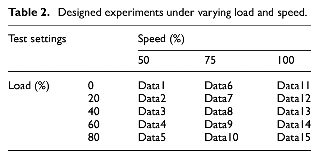
Figure 3(a) and (b) show the time domain plots of current and vibration signals for the healthy condition at different load and speed levels (Data1, Data8, and Data15). A slight fluctuation in the phase and amplitude of the current profile could be observed, while the vibration signals did not exhibit distinguishable change across the different load and speed conditions. However, the FFT spectra of the vibration signals revealed prominent changes in the magnitude and position of the harmonics as shown in Figure 3(c). Therefore, the distinct peaks and frequency components in the FFT data can be used as valuable features to capture the signal characteristics. The plots in Figure 4 show the time domain signals of current and vibration obtained for the healthy, misalignment, and outer bearing fault conditions. From the plots, it is evident that there is a substantial effect of these mechanical faults on the vibration signal, compared to the current profiles. The vibration signal under misalignment exhibited increased amplitude compared to the healthy state, with more pronounced fluctuations. The signal became even more irregular with larger spikes in the case of the outer bearing fault. However, the changes in the vibration signature did not follow a consistent pattern, appearing noisy and unpredictable. On the other hand, no significant differences in amplitude or waveform shape were observed in the current signals across the different fault conditions. This lack of clear, distinguishable features in the raw signals hinders their ability to accurately identify and diagnose faults. Therefore, advanced signal processing techniques are needed to extract meaningful features corresponding to different fault conditions.
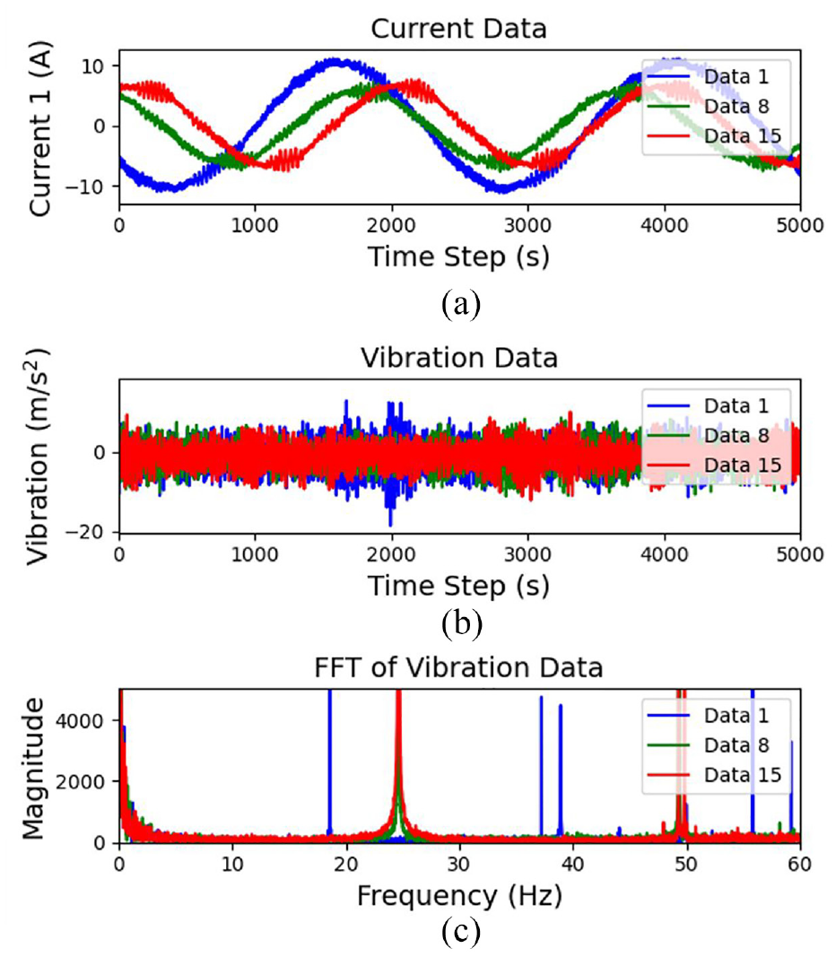
The healthy data obtained from different channels: (a) time-domain current 1 signal, (b) time-domain vibration (vertical) signal and (c) frequency-domain vibration (vertical) signal.
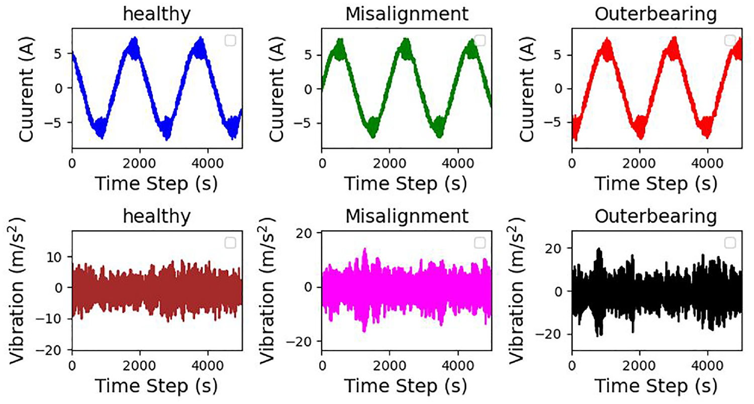
Current and vibration data under healthy, misalignment, and outer bearing fault conditions.
DL with 1D CNN and 2D CNN
CNN is a widely employed category of deep NNs, particularly effective in tasks related to image and video recognition. Broadly, the architecture of any CNN comprises the input layer, convolutional layer, pooling layer, and may include a fully connected layer and/or output layer, as illustrated in Figure 5. The input layer of a CNN is designed to accommodate time series signals in a standardized format suitable for 1D or 2D CNN utilization. However, before feeding raw data into a CNN model, various preprocessing steps are essential to optimize the data for accurate analysis. These steps include detrending, which removes underlying trends of the signals that might obscure critical patterns, and data scaling or normalization, which standardizes the range of variables, ensuring that no single feature dominates the model. Additionally, data slicing is employed to segment time series data into smaller portions using a sliding window technique, increasing the data size, and aligning with the input requirement of 1D and 2D CNN models.
43
The slicing window although selected systematically by trial and error has a profound impact on the model performance. As depicted in Figure 6, a slice or segment of each time-series signal, denoted as W, is chosen and organized horizontally for
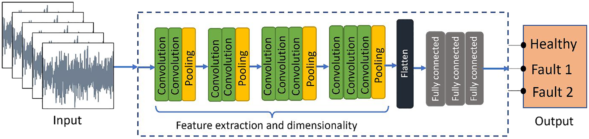
CNN architecture.
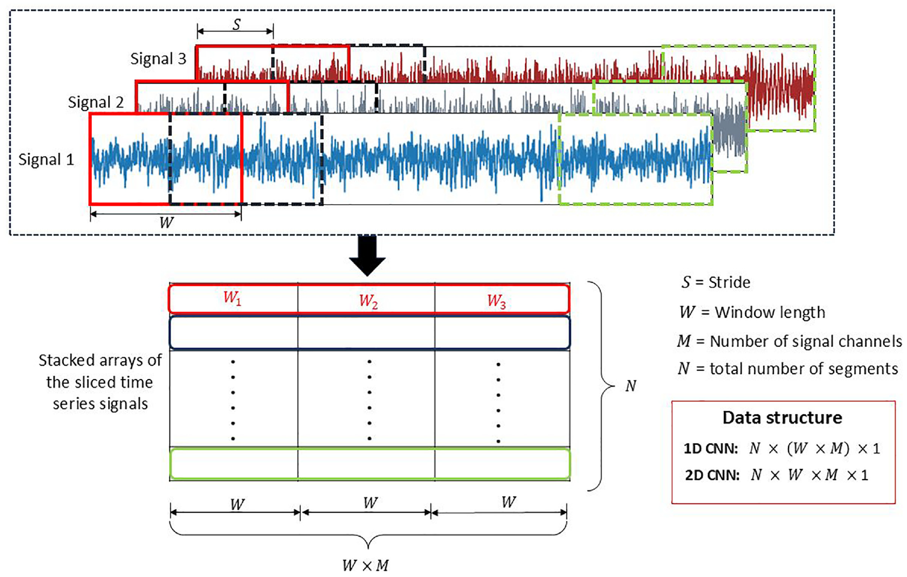
Data slicing. 23
For the 2D CNN application, a slight modification is made to the slicing algorithm, and the final data structure in this case is
The dataset was split into training and test sets with a train-test ratio of 7:3. The 70% training set is employed for training the CNN model, while the remaining 30% (i.e., the test dataset) is used for model validation.
In the convolutional layer, diverse filters are applied to the input data through a dot product operation (matrix multiplication), yielding feature maps. 17 These filters possess weights adjusted during training via a backpropagation algorithm to extract various features from the layer input.
The mathematical expression for convolution operation is
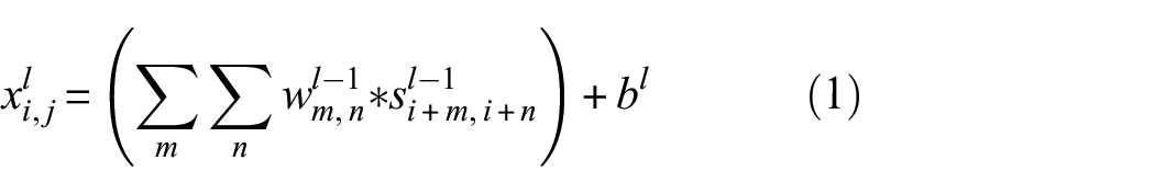
where
Following the convolution operation, the output
In the pooling layer, the spatial dimensions of the feature maps are decreased, aiming to reduce the model’s computation size and the risk of overfitting. 22 The resulting output of the pooling layer is flattened to ensure its depth is one, making it suitable for utilization in the fully connected layer. Additionally, the flattened output serves as the input for the fully connected layer, which operates as a standard feedforward network where neurons between two layers are interconnected. 15
Machine learning
Signal processing and feature extraction
Signal processing through FFT and DWT involves transforming time-domain signals into the frequency and time–frequency domain, respectively. Both FFT and DWT are valuable tools for feature extraction, but in most cases, they are not used simultaneously. In this study, FFT and DWT-based features were combined to capture the full spectrum of information across both frequency and time–frequency domains. The magnitude of the FFT harmonics obtained are used as the first set of features while the second set is obtained from the wavelet coefficients at each decomposition level. FFT provides a global frequency analysis, highlighting periodic components, while DWT captures localized features, offering information on nonstationary signal behaviors. This combined feature extraction approach consequently enhanced the sensitivity of the ML models to subtle anomalies and weak mechanical faults.
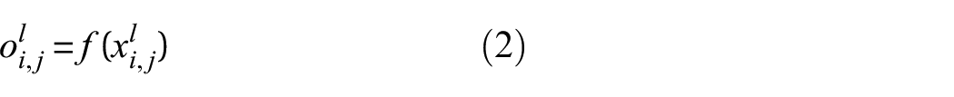
FFT is a long-existing tool for analyzing stationary signals (i.e., signals with unchanging spectral information over time). FFT is a method of representing a signal as a combination of a series of sine and cosine signals. A signal is transformed from the time domain to the frequency domain using FFT. The frequency spectrum produced by the FFT shows the amplitudes and phases of various frequency components of the input signal. Specific fault signatures or irregularities connected to various defects can be found by looking at the frequency spectrum. To characterize a fault, different features can be retrieved from the frequency spectrum obtained by FFT. The magnitudes of particular frequency peaks (see Figure 7), the presence of harmonics or sidebands, the spectral distribution, or other pertinent metrics are examples of these properties.
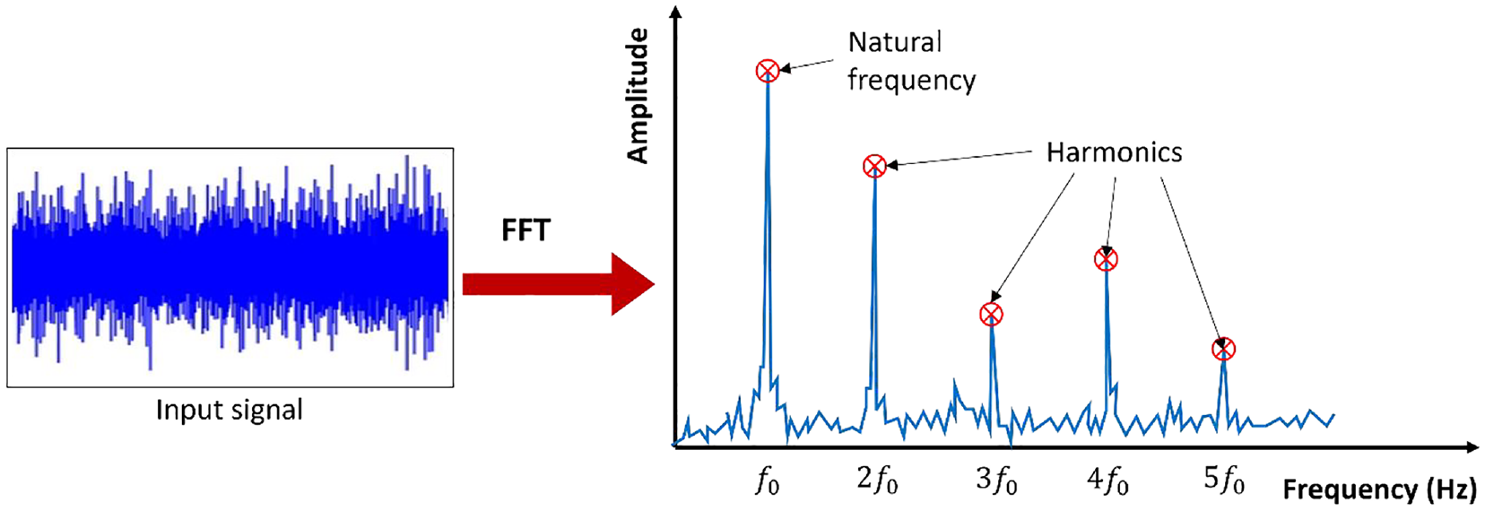
Schematic of FFT spectra indicating the natural frequency and harmonics.
Mathematically, FFT transforms the analyzed waveform X(t) with t samples into the frequency domain, represented by a finite number of frequency lines denoted as f. The separation between each line signifies the frequency resolution. The expression of FFT is presented in Equations (3) and (4). Figure 6 displays the typical FFT spectrum highlighting harmonics. These harmonics are characterized by being integer multiples of the natural frequency (f0) of the motor, presenting as clear peaks in the frequency domain at values like 2f0, 3f0, and so forth.
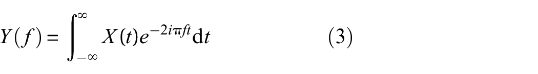
where

To address the challenge of information loss in either the time or frequency domain and achieve simultaneous optimal information from both domains, time–frequency analysis is employed. While STFT uses basic sine and cosine functions for time–frequency analysis, the WT stands out as a more sophisticated technique. WT utilizes a family of independently dilatable and shiftable elementary functions called wavelets. 46 Commonly used wavelet transform techniques include continuous wavelet transform (CWT), DWT, and wavelet packet transform. CWT is known for its redundancy in signal reconstruction, necessitating extensive computation time. Conversely, DWT provides sufficient information for original signal analysis with significantly reduced computation time. 47
The selection strategy of an appropriate wavelet function for analyzing nonstationary data in structural health monitoring was extensively discussed by Silik et al. 48 It was established that Daubechies (db) and Symlet (sym) wavelets, particularly order 3, demonstrated superior performance in denoising, feature extraction, and signal recovery accuracy. Furthermore, db3 outperformed other wavelets by showing low mean squared error and high SNR, and also exhibited a good balance between preserving signal energy and representing it sparsely. The “db” wavelet family had been used in other studies49,50 because of its distinct characteristics like smoothness, time–frequency localization, and vanishing moments over other mother wavelets like Haar and Symlet wavelets of the same order. It can effectively handle both sharp and smooth variations in signals, making it versatile for a wide range of applications such as feature extraction. Therefore, the “db3” wavelet was selected for the present analysis, with the decomposition performed up to 12 levels.
In DWT, a signal is broken down into several frequency sub-bands at various resolution settings. This is accomplished by passing the signal through several high-pass and low-pass filters. A set of approximation coefficients (low-frequency components) and detail coefficients (high-frequency components) at various scales are produced by the decomposition as illustrated in Figure 8. The high-frequency components of the signal are described by the detail coefficients from the DWT. These coefficients capture brief or sudden signal shifts, which are frequently an indicator of faults. Informative features can be extracted by looking at the statistical qualities or other traits of the detail coefficients. After DWT the signal undergoes decomposition into a tree structure, wherein each level of the signal is represented by detail (
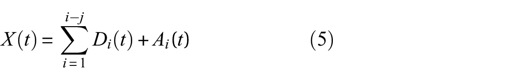
Different levels of DWT decomposition and extracted features.
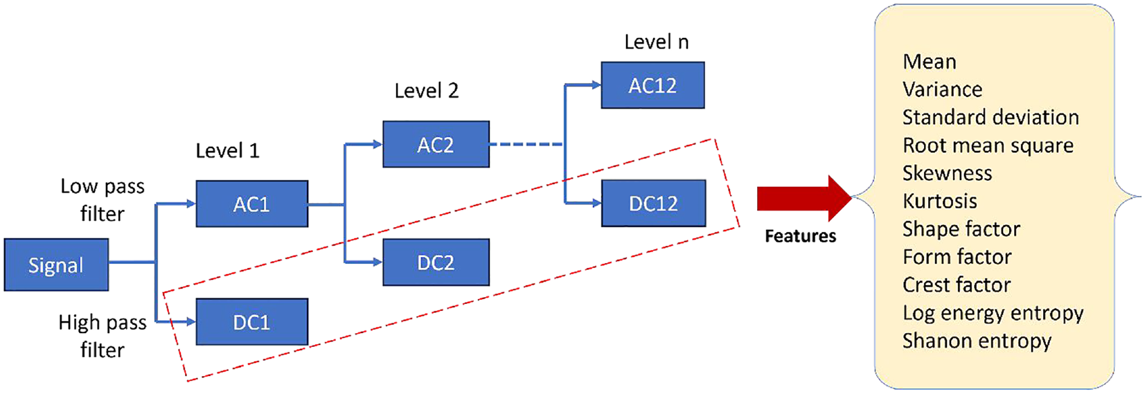
Not every particular coefficient might be important for identifying faults. Some coefficients might include noise or unrelated data. Techniques for feature selection can be used to find the coefficients that are most informative and discriminative. This may aid in lowering the dimensionality of feature space and enhancing classification precision. The formulas of the statistical, shape-based, and entropy features extracted from DWT-transformed signals are listed in Table 3.
Different features extracted from the vibration and current signals.
Random forest
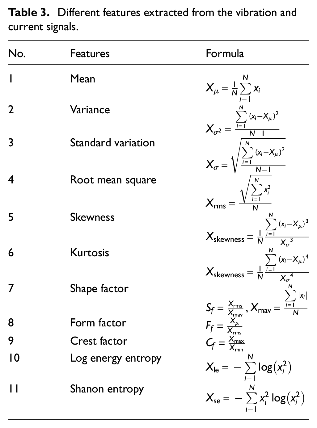
Random forest is a supervised ML technique that is built upon multiple decision trees and can be used for classification tasks. 51 Decision trees are simple yet a powerful type of ML model that recursively splits the dataset into subsets based on the most informative features to make predictions. RF uses random sampling, random feature selection, and a voting mechanism to ensure a stable and reliable prediction is attained; thus, overfitting is prevented. 3 Figure 9(a) diagrammatically shows the concept of the random forest algorithm. In classification tasks such as fault diagnosis of IM, the final output of an RF is the class that is chosen by the majority of the individual trees in the ensemble. RF has hyperparameters like the number of trees (n_estimators), the maximum depth of trees (max_depth), and the number of features to consider at each split (max_features). Tuning these parameters can greatly affect model performance.
Structure of (a) random forest and (b) XGBoost classifiers.
XGBoost
XGBoost, which stands for eXtreme Gradient Boosting, is a powerful and efficient ML algorithm that belongs to the gradient boosting family. Similar to RF, XGBoost is an ensemble learning method that combines the predictions of multiple weak learners (typically decision trees) to create a strong predictive model. XGBoost uses gradient boosting, which means it optimizes the loss function by iteratively adding decision trees to the ensemble as depicted in Figure 9(b). 3 Each tree is trained to minimize the residual errors of the previous trees. The final prediction in XGBoost is based on the weighted average of the predictions from all the trees, with more weight given to the trees that contribute more to reducing the error. Random Forest and XGBoost are ensemble learning methods that aim to improve predictive accuracy and reduce overfitting. However, they differ in the way they create and combine the individual models within the ensemble. Random Forest creates a set of independent decision trees and aggregates their results, while XGBoost builds a sequence of interrelated decision trees through the boosting process.
Results and discussion
The results obtained with the DL and ML techniques are presented in this section. The presented ML and DL models were trained using the TensorFlow DL framework on an Intel Core i7 1.80GHz CPU, 16-GB RAM, and an NVIDIA GeForce MX150 4GB GPU. Moreover, the approximated time taken for each model to predict the class of the test dataset is given in Table 4. The computational time result suggests that the ML models (RF and XGBoost) are relatively faster to run than the DL models (1D and 2D CNN), as the ML models rely on pre-engineered features. In comparison, the DL models extracted complex features from the sequential data but required multiple passes through the network layers. Interestingly, in all the models, the time required for processing vibration data was consistently lower compared to current data. This difference can be attributed to the more intricate frequency components and patterns present in current signals, especially under varying load and speed conditions, which demand additional processing time. However, all the ML and DL models demonstrated rapid test performance, with test times under 0.32 s, making them highly suitable for real-time applications.
The computational time of the models with the test datasets.
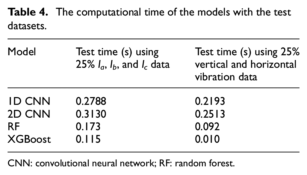
CNN: convolutional neural network; RF: random forest.
1D and 2D CNNs results
A simple 1D and 2D CNN architectures, each with two convolution layers, two pooling layers, one flattening layer, and two fully connected layers were developed as illustrated in Figure 10 and trained on the experimental data obtained as reported in the section “Experimental setup.” In both networks, the ReLU activation function is employed for the hidden layers, and the last layer in both architectures utilizes Softmax to determine the class of the outputs. The training hyperparameters are defined as follows: 20 epochs, 1000 batches, Adam optimizer, and categorical cross-entropy loss.
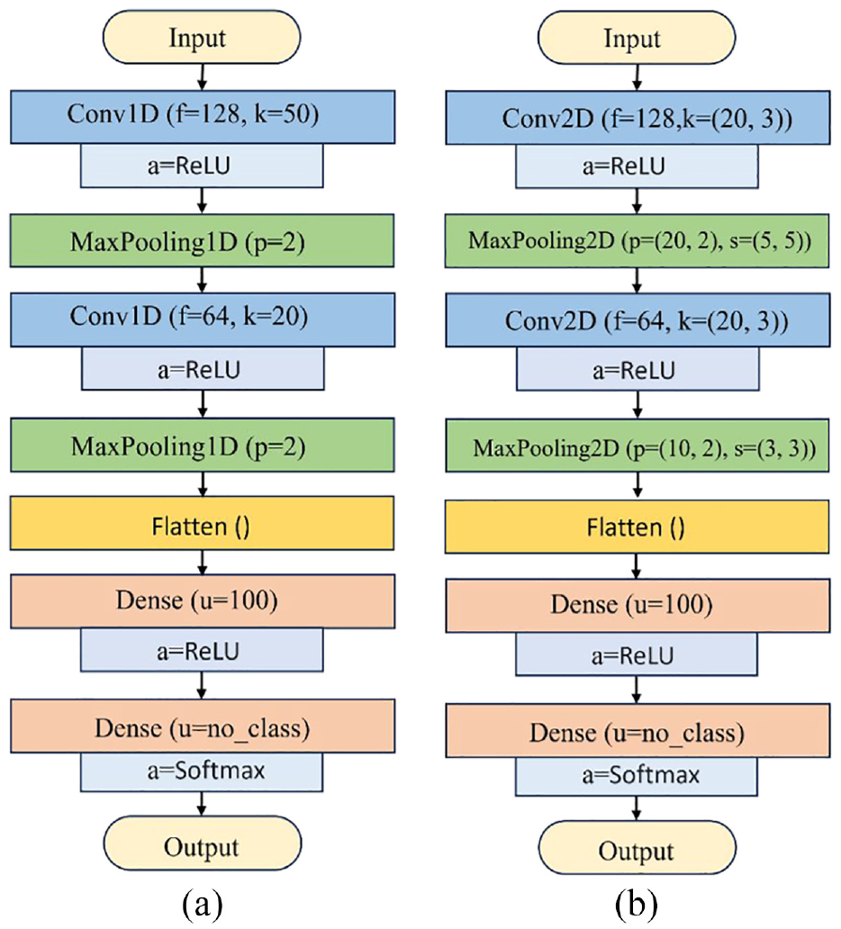
Structure of (a) 1D CNN and (b) 2D CNN models for IM fault diagnosis.
The results presented in Tables 5 and 6 show the test and validation accuracies obtained in the classification of the motor faults using 1D and 2D CNNs respectively. The results also include columns detailing the amount of training parameters and training time for each case. From Table 5, both 1D and 2D CNNs gave accuracies greater than 95% with the motor 2 vibration signals (i.e., the vertical and horizontal vibration from the motor housing). The t-distributed stochastic neighbor embedding (t-SNE) plot depicted in Figure 11 provides a low-dimensional representation of both the input and sixth layers of the CNN models. It reveals that the two models effectively learned the patterns associated with each fault when vibration signals were utilized. Results shown in Table 6 for the case of the three-phase current signals are unsatisfactory.
The performance of DL models with the motor 2 vibration signals.
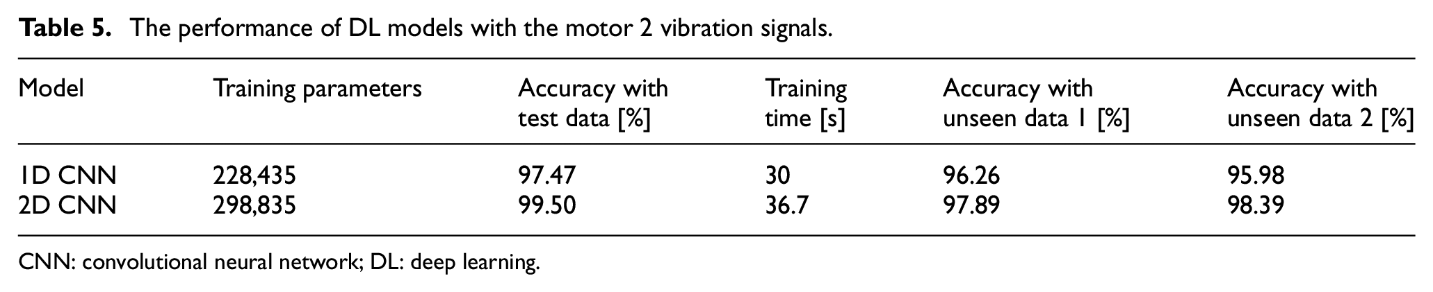
CNN: convolutional neural network; DL: deep learning.
The performance of CNN models with the motor 3 current signals (I a , I b , and I c ).
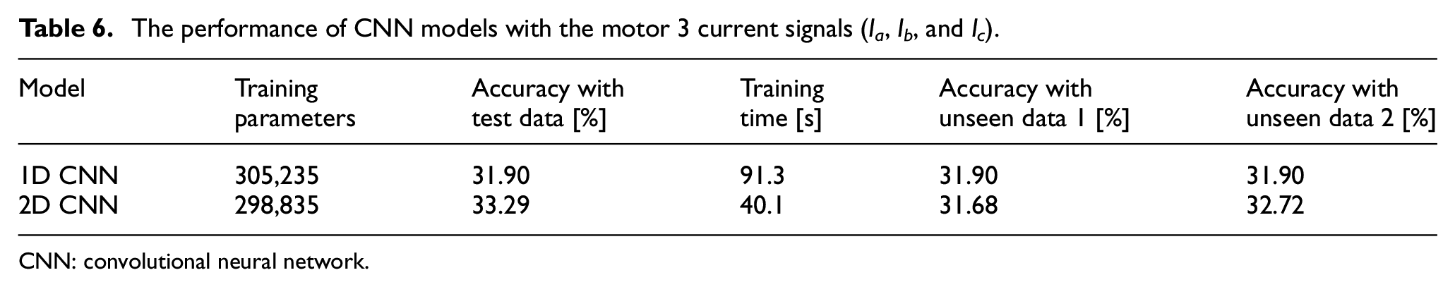
CNN: convolutional neural network.
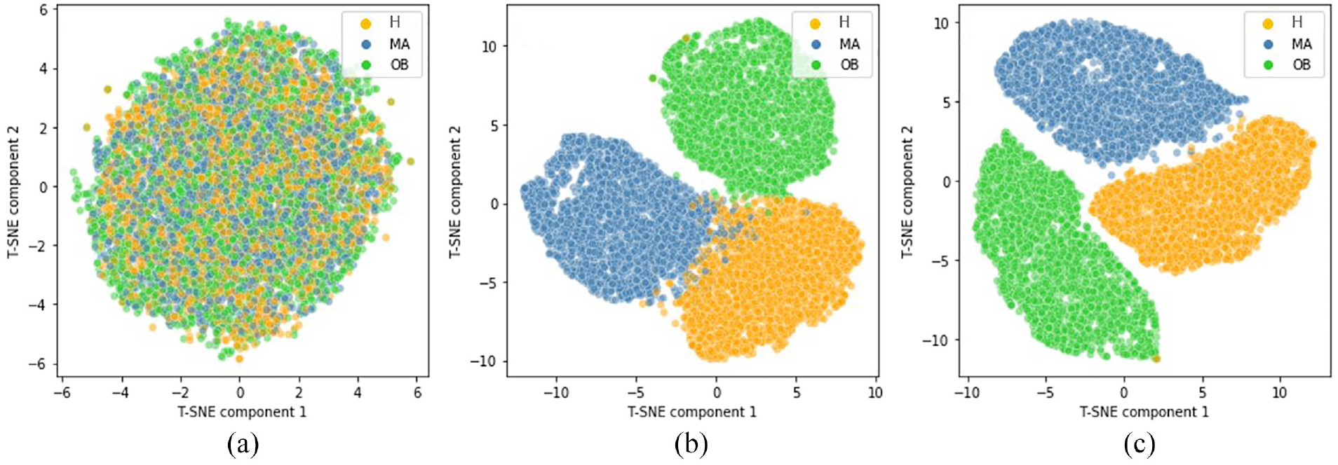
The t-SNE plot of the (a) raw data, (b) 1D CNN, and (c) 2D CNN.
RF and XGBoost results
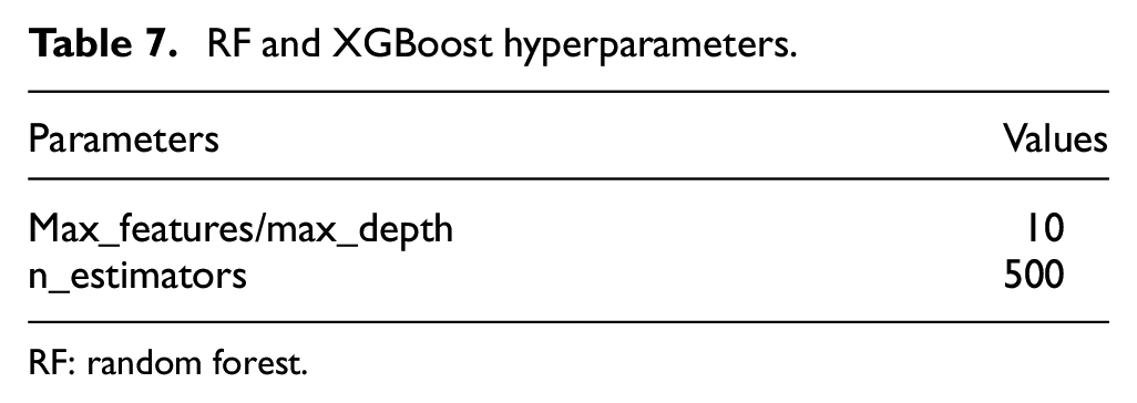
The RF and XGBoost ML models were trained using three distinct sets of features. The first set are the eight peaks derived from the FFT of signals as shown in Figure 12. Those peaks are the dominant peaks around the harmonics because the supply frequency is between 50 and 60 Hz. The second features are the 132 time–frequency features from DWT. The total number of the second features is high because 11 features are extracted from each of the 12 detailed coefficient signals generated after DWT. The third features come from the combination of the first and second features (140 in total). The number of features and the ML parameters were guided by the values employed in other similar works and further tuned by trial and error. The hyperparameters used in training the two ML models are listed in Table 7.
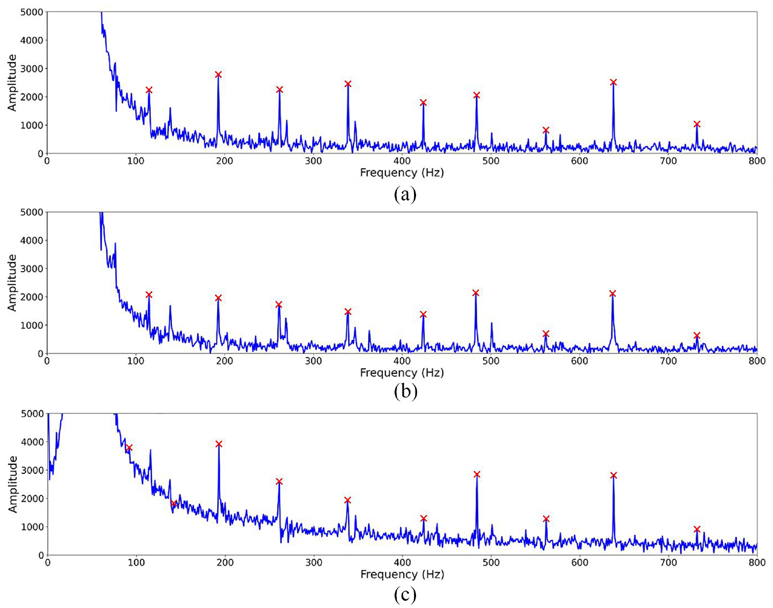
FFT plots of the current signal for (a) healthy, (b) misalignment, and (c) outer bearing fault conditions, and the selected harmonics.
RF and XGBoost hyperparameters.
RF: random forest.
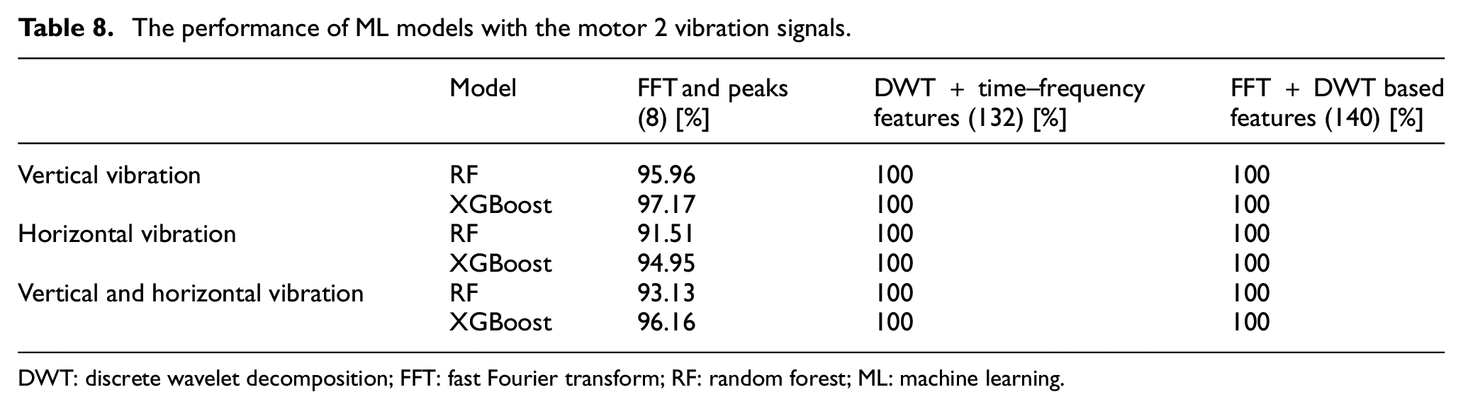
The performance of the ML models (RF and XGBoost) based on features computed from vibration and current signals are shown in Tables 8 and 9, respectively. From Table 8, when vibration signals are used, it is evident the classification accuracies of the two ML models are equal or close to 100% with the DWT-based features, as well as the combined features from FFT and DWT. However, the best classification accuracy when current signals are used was 87.41% from Table 9. The two reasons for the superior accuracy of the vibration signals are their sensitivity to mechanical faults and the provision of detailed frequency information with distinct patterns for each fault.
The performance of ML models with the motor 2 vibration signals.
DWT: discrete wavelet decomposition; FFT: fast Fourier transform; RF: random forest; ML: machine learning.
The performance of ML models with motor current signals.
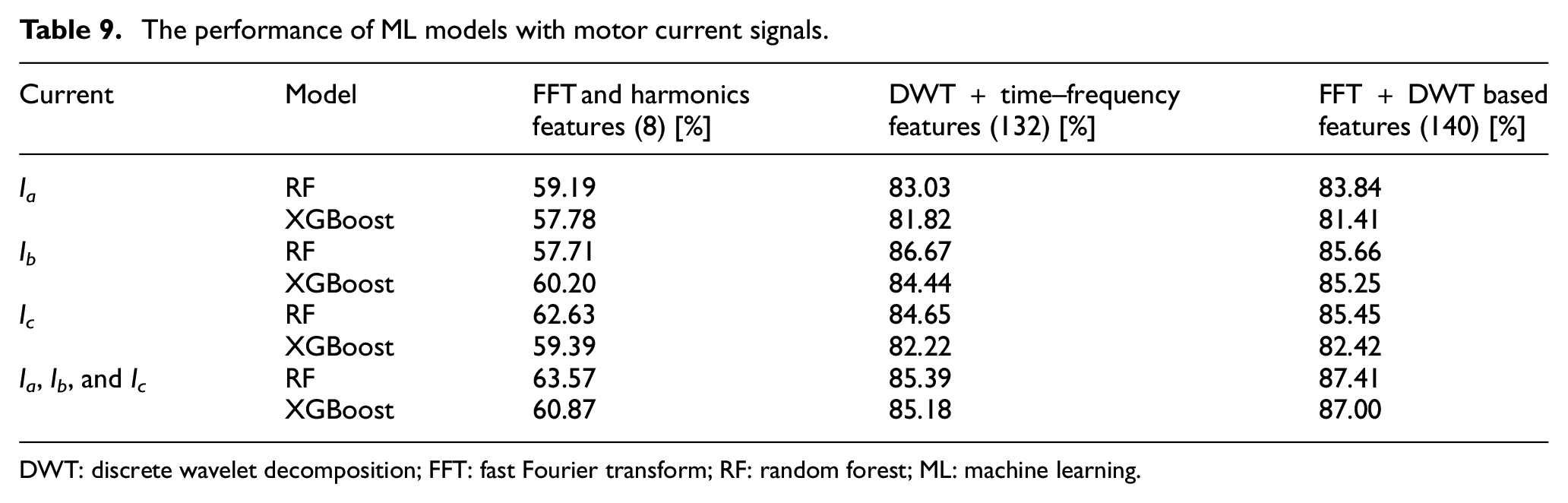
DWT: discrete wavelet decomposition; FFT: fast Fourier transform; RF: random forest; ML: machine learning.
Discussion
The comparison highlights the exceptional classification accuracy of deep CNN models, averaging 97% for unseen vibration data. Conversely, the performance diminishes significantly to an average accuracy of only 32% when using current signals. This disparity arises due to the susceptibility of current signals to electrical noise and interference. DL methods, particularly while dealing with raw current signals, face challenges in extracting clear patterns directly. The influence of induction motor operating conditions, such as load and transient states, further complicates current signal responses, potentially causing misinterpretation of fault signatures. In contrast, vibration signals, being primarily influenced by mechanical effects and less affected by electrical variations, offer more relevance.
Moreover, Figure 12 shows the FFT plot of current signals for both the healthy and fault conditions. From the figure, it is evident that the peaks of harmonics exhibit similarity, posing challenges in accurately distinguishing between individual faults. Hence, effective representation of fault characteristics in current signals requires advanced signal processing like DWT and manual extraction of relevant features.
After identifying dominant features, including the amplitude of FFT harmonics and DWT features, ML classifiers achieved significantly higher accuracy for current signals, averaging approximately 85% for both RF and XGBoost models. Specifically, ML models using FFT features alone exhibited an accuracy between 57% and 63%, and with only DWT features, approximately 84%. This underscores the richer information content of DWT features compared to FFT, as DWT provides excellent resolution in both time and frequency domains. Notwithstanding, the combination of FFT and DWT features gave the highest accuracy of 87.47% for the case of using the three current signals (I a , I b , and I c ) and the RF model. For vibration signals in ML models, a perfect accuracy of 100% was achieved, showcasing the highest sensitivity of vibration signals in detecting the investigated fault classes. Notably, with proper preprocessing, this article demonstrates the feasibility of obtaining satisfactory accuracy in fault detection for IMs using current signals, positioning them as a cost-effective alternative.
Conclusion
This study showed the performance of vibration and current signals in the classification of the state of an IM using DL (1D and 2D CNNs) and ML (RF and XGBoost) techniques. The comparative findings indicate that vibration signals demonstrate an exceptionally high level of accuracy, nearly reaching 100%, and they surpass current signals in detecting the studied mechanical faults. However, the highest accuracy achieved with the current signals was 87.41%, after performing signal processing and manual feature extraction, due to the weak and mechanical nature of the faults under investigation and the slight influence they have on the electrical signature of the IM.
Footnotes
Declaration of conflicting interests
The author(s) declared no potential conflicts of interest with respect to the research, authorship, and/or publication of this article.
Funding
The author(s) received no financial support for the research, authorship, and/or publication of this article.