Sage Journals: Discover world-class research

Abstract

Condition assessment of water transmission pipelines is of important necessity for prioritizing rehabilitation and preventing catastrophic pipe failure. Hydraulic transient analysis has been investigated for three decades for this purpose and applied to many field studies. However, the significant pipe vibrations caused by the transient generation process and the limited energy and bandwidth of conventional discrete transient pressure waves (e.g., step and pulse waves) limit the accuracy and resolution of the analysis. This paper reports a pilot field study of noninvasive and nondestructive pipe condition assessment using small amplitude and persistent hydroacoustic noise instead of conventional large and discrete hydraulic transient waves. By opening a discharge valve installed at an existing access point, such as an air valve, on the field pipe, hydroacoustic noise was generated at the valve due to the turbulence of the discharge. The hydroacoustic noise was measured by pressure transducers at this access point as well as some other access points along the field pipe. A signal deconvolution process was then applied to the measured hydraulic pressures to transfer them to a compositional impulse response function (IRF), which is composed of IRFs of different pipe sections. A mathematical model was derived to interpret the anomaly-induced spikes on the deconvolution trace. A time-shifting process on the compositional IRFs was proposed to find the locations with pipe condition changes from a specific direction of the pipe. The field study has shown that small-amplitude persistent hydroacoustic noise can replace conventional large hydraulic transient waves for pipe condition assessment.

Keywords

Asbestos cement pipe hydraulic transient hydroacoustic waves impulse response pipe condition assessment

Introduction

Different techniques, such as vibration-based inspection using entropy measures,¹ guided wave ultrasonics,^2,3 acoustic emission,⁴ and hydraulic transient-based techniques⁵ have been proposed for pipeline structural assessment in the past decades. These methods are promising in field application because they are noninvasive, nondestructive, and efficient for long pipes. Typically, discrete hydraulic transient pressure waves are generated by abruptly operating a side-discharge valve, resulting in step or pulse pressure waves. The transient pressure including the incident wave and the transient reflections are collected by high-speed pressure sensors. Based on analyzing the transient reflections in the time domain or specific features in the frequency domain, pipe discontinuities such as leaks,^6–9 discrete (partial) blockages,^10,11 extended blockages,^12–16 pipe wall deterioration, and corrosion^17,18 can be determined.

In the past two decades, several field tests have been conducted to validate the transient-based pipe condition assessment techniques. On a long mild-steel concrete-lined pipeline, Misiunas¹⁹ conducted field tests to detect a single leak, multiple leaks, air pockets, and discrete blockage by examining the difference between the measured transient pressure in an intact pipe and the pressure measured in the pipe with the anomalies added. The approach needs a reference transient pressure trace corresponding to an intact pipe before the anomaly occurs, which limits its application. On the same pipe system, hydraulic transient tests were conducted to determine continuous pipeline wall thickness variations due to internal pipe corrosion and cement mortar lining loss.²⁰ The measured transient pressure traces were used in an inverse transient analysis, which incorporates an inverse search algorithm to analyze patterns of measured pressure reflections. On an asbestos cement (AC) pipeline, similar field transient tests were conducted with typically one location for transient generation and multiple places for pressure measurements.²¹ A sub-sectional condition assessment method was used to achieve an efficient condition assessment that provides average wave speed and wall condition of each of the sub-sections bounded by two pressure measurements. Field transient tests were also conducted in pipe networks with a single device to generate a mild transient and to collect the transient pressure at a fire hydrant.²² The transient pressure was transferred to the frequency domain to obtain the cepstrum, which is defined as the Fourier transform of the logarithm of the Fourier transform of a signal in the time domain. By repeating the transient tests and averaging the calculated cepstra obtained from each test, the averaged cepstra were then used to localize leaks in the pipe network.

To apply transient-based pipe condition assessment techniques, suitable incident pressure waves are needed to excite the pipeline system. Generating incident pressure waves with sufficient bandwidth and energy is a challenge. Typically, a discharge valve controlled mechanically can create transient pressures with a duration of several milliseconds in laboratory pipes¹⁸ and tens of milliseconds or more in field pipes.²⁰ Other transient generators have been developed for condition assessment, such as the spark transient pressure wave generator which can generate sharp pulses with a duration of approximately 0.1 ms in laboratory pipes.²³ Large transient pressure waves caused by pump trips were used for anomaly prelocalization in distribution–transmission mains.²⁴ Another challenge of the transient-based techniques is the background noise in the pipe system, which may be misinterpreted as wave reflections from pipe defects.²⁵ To reduce the effects of the background noise, the magnitude of the transient pressure typically needs to be large (several meters or more), which may cause large pipe vibration and strong fluid-structure interaction.^26,27

Compared with conventional hydraulic transient pressure waves, hydroacoustic waves are normally of a much smaller magnitude and may be generated persistently in a pipe. Since they are persistent, the signal-to-noise ratio can be very high even though the magnitude of the waves is very small. The method to generate hydroacoustic waves in water pipes can be easy and convenient, such as opening a discharge valve to generate discharge noise (like leak noise). Thus, complex and customized transient generators are not needed anymore in hydroacoustic tests. In the field, hydroacoustic tests and analysis are normally used for passive detection, such as passively listening to leak noise to detect leaks.²⁸ Limited research has been conducted on proactive methods using hydroacoustic waves in the field.

Hydroacoustic noise was used in the laboratory on a single copper pipe²⁹ and then on a pipe network updated from the single copper pipe for proactive anomaly detection.³⁰ In these laboratory tests, a signal deconvolution process using a least-squares deconvolution approach³¹ was applied to the pressures measured at two locations on the pipe. This resulted in specific impulse response function (IRF) traces for different system configurations. Mathematical models were developed to interpret the spikes on the IRF traces and to link these spikes to anomalies in the pipe system. However, when such methods are applied in the field where ideal access points for the sensors and the discharge are not available and wave dissipation may be significant, the developed mathematical models may be problematic. Other factors such as the standpipes where the pressures are measured in the field, and the wave dissipation in the pipe with a much larger diameter than those in the laboratory may need to be considered in the analysis.

The current paper reports a field study on proactive pipe condition assessment using hydroacoustic noise generated by a partially open side-discharge valve. Similar to the previous laboratory studies,³¹ a signal deconvolution process is applied to the preprocessed pressures measured at two standpipes connected to the main pipe at different locations. To interpret the spikes on the resultant IRF traces, a mathematical model incorporating the transmission and reflection by the standpipe is developed. A time-shifting process is then applied to the IRFs to clarify the directions of the wave reflections. The results using the hydroacoustic noise are compared with the results using traditional hydraulic transient waves, which illustrates that hydroacoustic waves can replace traditional hydraulic transient waves in the field for pipe condition assessment.

Compositional impulse response function

In this section, a compositional IRF, which can be obtained from the hydroacoustic noise is derived and it is used to interpret the discontinuities in the pipeline. A time-shifting process is introduced, and it facilitates the unidirectional condition assessment. In the following section, the non-italic symbols represent physical locations, and the italic symbols represent parameters.

Pressure deconvolution

A typical field test configuration for hydraulic transient-based pipe condition assessment is shown in Figure 1. Pressure transducers are normally installed on a standpipe connected to the pipe main of interest in the field. Water is discharged from the middle standpipe through its open end. Conventionally, a transient generator installed at the end of the standpipe is abruptly closed to stop the discharge and thus generate a large pressure surge (a step wave). In this study, instead of using the large transient pressure step wave generated by valve closure, the discharge-induced hydroacoustic noise is used for pipe condition assessment.

Figure 1.

Schematic of the field test configuration.

The impulse responses of the pipe main at the left side and right side of the junction J_G are defined as $R_{L}$ and $R_{R}$ , respectively. The impulse responses of the pipe main at the left side of J₁ and the right side of J₂ are defined as $R_{L 1}$ and $R_{R 2}$ , respectively. The transfer function between J₁ and J_G is defined as $H_{1}$ and that between J₂ and J_G is defined as $H_{2}$ . The radius and the cross-sectional area of the standpipe are $r_{1}$ and $A_{1}$ and those for the pipe main are $r_{2}$ and $A_{2}$ . For a wave transmitting from the standpipe to the pipe main, the transmission ratio is

s_{1} = \frac{2 A_{1}}{A_{1} + 2 A_{2}}

(1)

For a wave transmitting from the pipe main to the standpipe, the transmission ratio is

s_{2} = \frac{2 A_{2}}{A_{1} + 2 A_{2}}

(2)

Since the length of the standpipe is much shorter than the pipe main, the length of the standpipe is neglected in this study. The transient or acoustic waves propagating along the pipe will be reflected by any anomalies in the pipes multiple times. The higher-order wave reflections are normally of much smaller magnitude compared with the principal wave reflections. To make the mathematical derivation concise, only the principal wave reflections are considered. The mathematical analyses of the pressure deconvolution between $P_{2}$ (Pressure at P_2) and $P_{G}$ (Pressure at P_G) is the same as between $P_{1}$ (Pressure at P_1) and $P_{G}$ and thus only the analysis of the pressure deconvolution between $P_{2}$ and $P_{G}$ is presented in the following.

For the pressure P_G, the major component is the generated hydroacoustic noise $P_{0}$ . With $P_{0}$ transmitting to the pipe main, the transmitted component is $P_{0} s_{1}$ . The wave reflections coming from the left side and the right side to the point J_G are $P_{0} s_{1} R_{L}$ and $P_{0} s_{1} R_{R}$ , respectively. After transmitting to P_G, the wave reflections become $P_{0} s_{1} R_{L} s_{2}$ and $P_{0} s_{1} R_{R} s_{2}$ , and thus the total pressure P_G is

P_{G} = P_{0} + P_{0} s_{1} s_{2} R_{L} + P_{0} s_{1} s_{2} R_{R}

(3)

For the pressure P_G, the hydroacoustic noise $P_{0} s_{1}$ and the wave reflections from the left side of J_G, $P_{0} s_{1} R_{L}$ , will propagate to point J₂ and then to P₂ and thus become $P_{0} s_{1} s_{2} H_{2}$ and $P_{0} s_{1} s_{2} R_{L} H_{2}$ , respectively. By assuming the impulse response from the right side of J₂ as $R_{R 2}$ , the wave reflections from the right side become $P_{0} s_{1} H_{2} R_{R 2}$ at point J₂ and thus $P_{0} s_{1} s_{2} R_{R 2} H_{2}$ at P₂. As a result, the total pressure at P₂ is

P_{2} = P_{0} s_{1} s_{2} H_{2} + P_{0} s_{1} s_{2} R_{L} H_{2} + P_{0} s_{1} s_{2} R_{R 2} H_{2}

(4)

Assuming $s = s_{1} s_{2}$ , the division between $P_{2}$ and $P_{G}$ gives

\frac{P_{2}}{P_{G}} = H_{2} s (\frac{1 + R_{L} + R_{R 2}}{1 + s R_{L} + s R_{R}})

(5)

By applying a Taylor series expansion to the denominator and considering the principal wave reflections, Equation (5) can be manipulated to

\frac{P_{2}}{P_{G}} = H_{2} s (1 + R_{L} + R_{R 2} - s R_{L} - s R_{R})

(6)

which can be rewritten as

\frac{P_{2}}{P_{G}} = H_{2} s [1 + (1 - s) R_{L} + R_{R 2} - s R_{R}]

(7)

If the pressure transducers are directly connected with the pipe main,³² then $s = 1$ and thus

\frac{P_{2}}{P_{G}} = H_{2} (1 - R_{R} + R_{R 2})

(8)

This is exactly the same as the first-order wave decoupling equation reported by the authors before.³² The equation can be further simplified to the paired-IRF equation²⁹ by assuming a uniform section between two standpipes. For these situations, the pressure deconvolution will only examine one side of the pipe each time.

Similar to the analysis of the pressure deconvolution $P_{2} / P_{G}$ , the pressure deconvolution $P_{1} / P_{G}$ can be written as

\frac{P_{1}}{P_{G}} = H_{1} s [1 + (1 - s) R_{R} + R_{L 1} - s R_{L}]

(9)

Based on Equations (7) and (9), it can be concluded that the pressure deconvolution will result in a compositional IRF that contains individual IRFs of several different sections of the pipeline. For any discontinuity in the pipeline, a spike will occur on the individual IRF and multiple spikes may occur on the compositional IRF if the individual IRFs have overlaps, such as $R_{R 2}$ and $R_{R}$ in Equation (8). In the following, the compositional IRF obtained from $P_{1} / P_{G}$ is defined as IRF₁, and that obtained from $P_{1} / P_{G}$ is defined as IRF₂.

From Equations (7) and (9), it shows that the diameter of the standpipe has a significant effect on the magnitude of the spikes in the compositional IRFs. A small diameter of the standpipe will lead to a small value of s which will overall reduce all the spikes due to the term $H_{1} s$ in front of the brackets. By normalizing the compositional IRF to make the incident spike to unity, the effect can be eliminated. A small diameter of the standpipe can also reduce the magnitude of spikes in $s R_{R}$ in Equation (7) and $s R_{L}$ in Equation (9), which contains virtual spikes that will be discussed in the field test analysis.

Theoretically, the wave reflection coefficient, which is the reflection ratio at a discontinuity, can be estimated by

r = \frac{B_{2} - B_{1}}{B_{2} + B_{1}}

(10)

where B is the characteristic impedance of a pipe section. The subscripts 1 and 2 represent the pipe sections before the impedance change and after the change, respectively. The characteristic impedance can be calculated by

B = \frac{a}{gA}

(11)

where g is acceleration of gravity, A is the internal cross-section area of the pipe section and a is the wave speed in the pipe section. It should be noted that the wave dissipation and dispersion in the pipe section will diminish the IRF coefficient significantly in the field.

Time-shifting the IRFs to overlap anomaly-induced spikes

Normally, the diameter of the pipe main is much larger than that of the standpipe, and the area ration $A_{1} / A_{2}$ will be of a small value. This will lead to a small value of s, normally less than 0.15. Thus, the term $R_{L}$ in Equation (9) and $R_{R}$ in Equation (7) will be significantly diminished. In the following analyses, the term $R_{L}$ in Equation (9) and $R_{R}$ in Equation (7) will be neglected and the effects of these two terms will be discussed specifically later in the field test analysis.

The relationships between different IRFs are

R_{L} = H_{1}^{2} R_{L 1}

(12)

R_{R} = H_{2}^{2} R_{R 2}

(13)

By substituting Equations (12) and (13) into Equations (7) and (9), the pressure deconvolutions can be written as

\frac{P_{1}}{P_{G}} = H_{1} s + s (1 - s) H_{1} H_{2}^{2} R_{R 2} + s H_{1} R_{L 1}

(14)

\frac{P_{2}}{P_{G}} = H_{2} s + s (1 - s) H_{1}^{2} H_{2} R_{L 1} + s H_{2} R_{R 2}

(15)

It can be seen from Equations (14) and (15) that both equations contain $R_{L 1}$ and $R_{R 2}$ but multiplied by different transfer functions. Physically, the transfer functions $H_{1}$ and $H_{2}$ represent the wave dissipation, dispersion, and time delay by the wave traveling time in the section from J₁ to J_G and the section from J₂ to J_G, respectively. These time delays are defined as $τ_{1}$ and $τ_{2}$ . Thus, the time delay for $R_{R 2}$ in Equation (14) is $τ_{1} + 2 τ_{2}$ , while it is $τ_{2}$ for $R_{R 2}$ in Equation (15). The time delay for $R_{L 1}$ in Equation (14) is $τ_{1}$ , while it is $2 τ_{1} + τ_{2}$ for $R_{L 1}$ in Equation (15). By delaying the IRF₁ by $τ_{1} + τ_{2}$ , the spikes in $R_{L 1}$ in Equations (14) and (15) will match in time. Similarly, the spikes in $R_{R 2}$ in both IRFs can match together if IRF₂ is delayed by $τ_{1} + τ_{2}$ .

Field pipe system and tests

Field work was undertaken in Victoria, Australia in 2014 on a regional AC transmission main as shown in Figure 2.³³ The pipeline extended for over 9 km from a T-junction with a 375 DICL pipe. The water storage tank at the other end was isolated from the system by closing the inline valve at the entrance of the tank. The pipeline had several material and diameter changes with details shown in the schematic. GPS coordinates were gathered during the tests and were used to determine the chainages of the testing points as shown in Figure 2.

Figure 2.

Layout of the field pipe system.

The field tests were originally designed to validate the pipe condition assessment techniques using conventional step transient pressure waves. Step transient pressure waves were generated in the pipeline by establishing a side discharge through the transient generator at the air valve or hydrant point and then abruptly stopping this flow. Figure 3 shows a typical generation point, measurement point, and the data acquisition system (DAQ).

Figure 3.

(a) Transient generator attached to air valve, (b) measurement point, and (c) data acquisition system.

At the generation point, a check valve-based transient generator and a pressure transducer were installed on the standpipe connected to the pipe main. At the measurement point, a single pressure transducer (Druck PDCR 810 high-integrity silicon flush-mounted diaphragm transducer) was installed. The sampling frequency of the DAQ system for measuring pressure data was 2 kHz. Each DAQ system contained a GPS unit for time synchronization. Before the tests, air was bled through the bleeding valve installed at each measurement station as shown in Figure 3(b). This is to eliminate the impact of accumulated air bubbles at the measurement station on the measured pressure trace. The tests consisted of three major steps, starting from measuring the background pressure fluctuations and noise with the side discharge closed. This was then followed by a period of 2–3 mins to measure the hydroacoustic noise induced by the water discharge after opening the discharge valve. The magnitude of the hydroacoustic noise can be adjusted by changing the opening and the required magnitude is determined by the background noise interference and the wave attenuation. The last step is the traditional hydraulic transient test by suddenly closing the side-discharge valve. This will cause a sharp water hammer wave propagating along the pipe.

Tests were conducted along the pipeline with normally one generation point and two measurement points adjacent to the generation point. In the paper, one case with the generator located at point 12 (G) and measurement stations located at points 8 (M1) and 13-1 (M2) was selected for analysis. The pressure traces at the generation and measurement points are shown in Figure 4. It shows from the pressure traces that the background fluctuations and noise were measured before approximately 50 s, after which the check valve was opened and the hydroacoustic noise was measured. At approximately 330 s, the check valve was suddenly closed and induced large transient pressures. At the generation point, the pressure variation after the valve closure exceeds the measurement range of the transducer which was from 0 to 245 m.

Figure 4.

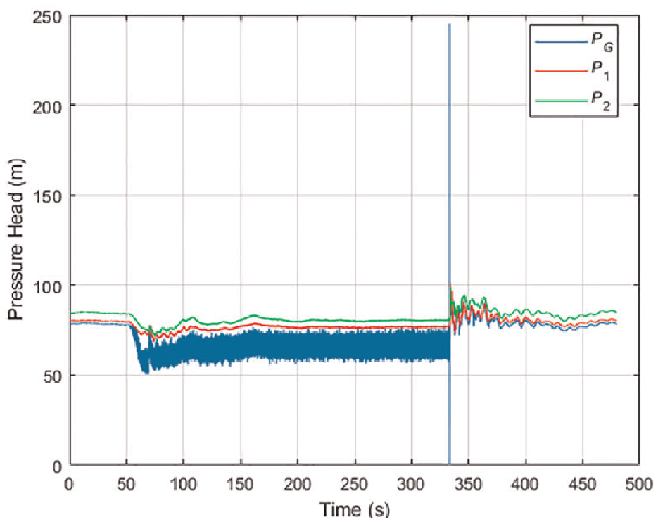
Measured pressure traces with the check valve opening at approximately 50 s and closing at approximately 330 s.

Data analyses

Signal filter

In this section, the hydroacoustic noise signals were selected by truncating the pressure signals in Figure 4, starting from 100 s with a window length of 200 s. The power spectral densities (PSDs) of the three pressure traces are shown in Figure 5. As can be seen from the figure, the PSD of the hydroacoustic noise at the generation point has a wide spectrum. However, the PSDs of the signals P₁ and P₂ show that the majority of the energy is concentrated below 100 Hz, which indicates strong attenuation at frequencies above 100 Hz. The statement can be also confirmed by the coherence plots between the hydroacoustic noise at the generation point and that at the measurement points as shown in Figure 6. The coherence value for both curves in Figure 6 drops quickly above 100 Hz and the signals are noncoherent above 170 Hz. By looking at the PSDs of these signals, it can be observed that some resonance peaks at 62–86 Hz, 216–225 Hz, and 432–438 Hz were identified on the PSD of the signal P₁ but not found on the other signals. These resonance peaks can be ascribed to the effects of the standpipe at the M1 measurement point and need to be eliminated from the signal for further signal analyses.

Figure 5.

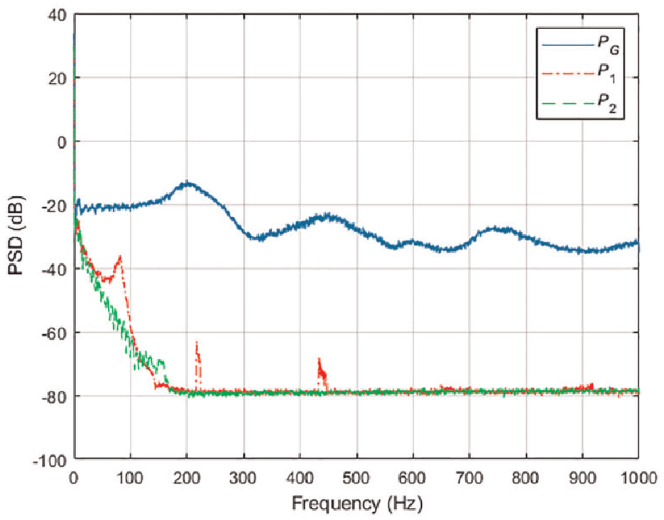
Power spectral densities for the hydroacoustic noise from 100 to 300 s.

Figure 6.

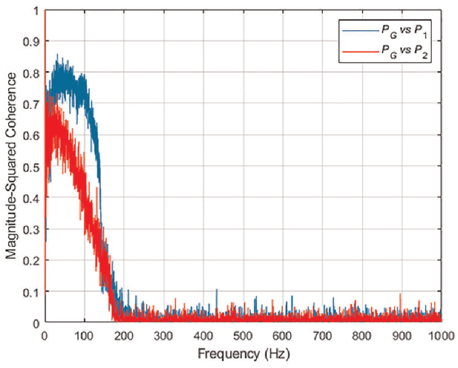
Coherence between the hydroacoustic noise at the generation point and the hydroacoustic noise at the measurement points.

To obtain useful signals from the raw pressure measurements, a bandpass Wavelet filter has been applied to the signals with a frequency band from 0.1 to 50 Hz. The filtered signals after normalization in a period of 60 s are shown in Figure 7.

Figure 7.

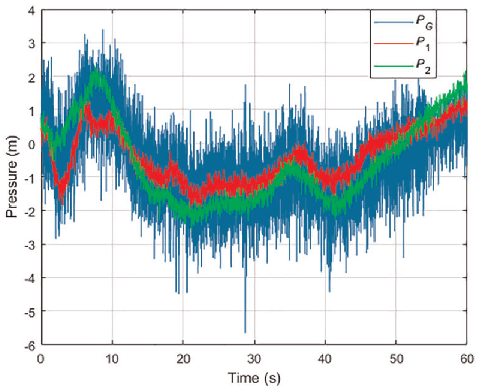
Filtered hydroacoustic noise from 100 to 160 s.

Signal deconvolution

As shown in Equation (7), the deconvolution between the pressure at the measurement points and the pressure at the generation point will lead to a combination of IRFs of the pipe system at different regions. The deconvolution in the time domain is equivalent to a division process in the frequency domain as

R (j ω) = Y (j ω) / X (j ω)

(16)

where $R (j ω)$ , $Y (j ω)$ and $X (j ω)$ are the Fourier transforms of the IRF, output and input of the deconvolution, respectively, j is the imaginary unit and ω is the angular frequency. Since the denominator $X (j ω)$ can tend to zero at high frequencies, leading to a singular inversion problem, the least-squares deconvolution in the time domain is applied as

R = (X^{T} X + λ I)^{- 1} X^{T} y

(17)

where $X$ is a lower triangular matrix consisting of the input elements (signal at G in this paper) and with rows being incrementally delayed vectors of the input, the column vector $y$ consists of the output time series at M1 or M2 in this case, the column vector $R$ is the time-domain series of the IRF coefficients, $I$ is the identity matrix, and λ is a positive constant parameter, which can be adjusted to determine the suppression level of the noise. Details of the least-squares deconvolution can be found in a previous publication.³¹ It should be noted that many other deconvolution techniques can also be used to calculate the IRF, and the least-squares deconvolution is used here as an example.

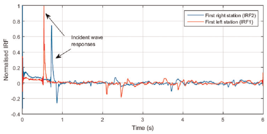
By using the hydroacoustic noise shown in Figure 7 and the least-squares deconvolution shown in Equation (17). The pressure trace P₁ is assigned to y, and the pressure trace P_G is assigned to x which will be used to generate the matrix X. Then the pressure deconvolution between P₁ and P_G can be obtained. A similar process was applied to P₂ and P_G. These two deconvolution traces IRF₁ and IRF₂ after normalization by dividing the IRF trace by the magnitude of the highest spike are shown in Figure 8.

Figure 8.

Normalized IRFs obtained from signal deconvolution.

As shown in Equations (14) and (15), the peak responses in IRF₁ and IRF₂ indicate the incident waves that propagate from the generation point to the measurement points. The occurring times of these spikes, $τ_{1}$ = 0.528 s and $τ_{2}$ = 0.714 s, correspond to the time taken by the wave to travel from G to M1 and M2, respectively. Given the distances from G to M1 and M2 are 599 m and 807 m, the wave speeds in these two sections are calculated as 1134 and 1130 m/s. An average wave speed of 1132 m/s is selected for this type of pipe in the following analysis.

To validate the accuracy of the reflection ratio in the following analyses, the wave speed of the 300 DICL pipe section was calibrated through another test with the water discharge at point 18 and measurements at points 15 and 20 in Figure 2. The wave traveling times for the incident waves were obtained as 0.777 and 0.528 s, corresponding to the distances of 933 and 630 m. The wave speeds are calculated as 1201 and 1193 m/s, and an average of 1197 m/s is selected for this type of pipe.

Time-shifting the IRFs to overlap anomaly-induced spikes

The internal diameter of the standpipe is 75 mm while the diameter of the pipeline is 225 mm. The ratio of the cross-sectional area of the standpipe to that of the pipeline is 1:9. The transmission ratios $s_{1}$ and $s_{2}$ in Equations (1) and (2) can be then calculated as $2 / 19$ and $18 / 19$ , respectively, which leads to a small value of 0.1 for the parameter s in Equation (5). Thus, the spikes in $R_{L}$ in Equation (9) and those in $R_{R}$ in Equation (7) will be significantly diminished and the focus will be given on other individual terms in IRF₁ and IRF_2.

To validate the effectiveness of condition assessment using the compositional IRFs obtained from the hydroacoustic noise, the conventional transient-based assessment method using large transient pressure surges was also applied in the following analyses. Similar to the process of delaying the IRFs, the delaying process was also applied to the large transient pressure waves to localize anomalies unidirectionally. By delaying the transient pressure wave $P_{1}$ by $τ_{1} + τ_{2}$ and matching with the original transient wave $P_{2}$ , the condition of the pipe section at the left side of M1 can be examined. By delaying the transient pressure wave $P_{2}$ by $τ_{1} + τ_{2}$ , and matching with the original $P_{1}$ , the condition of the pipe section at the right side of M2 can be examined. The details of the time-shifting method using transient pressure waves were reported with field test validation.²¹

(a) Left side of M1

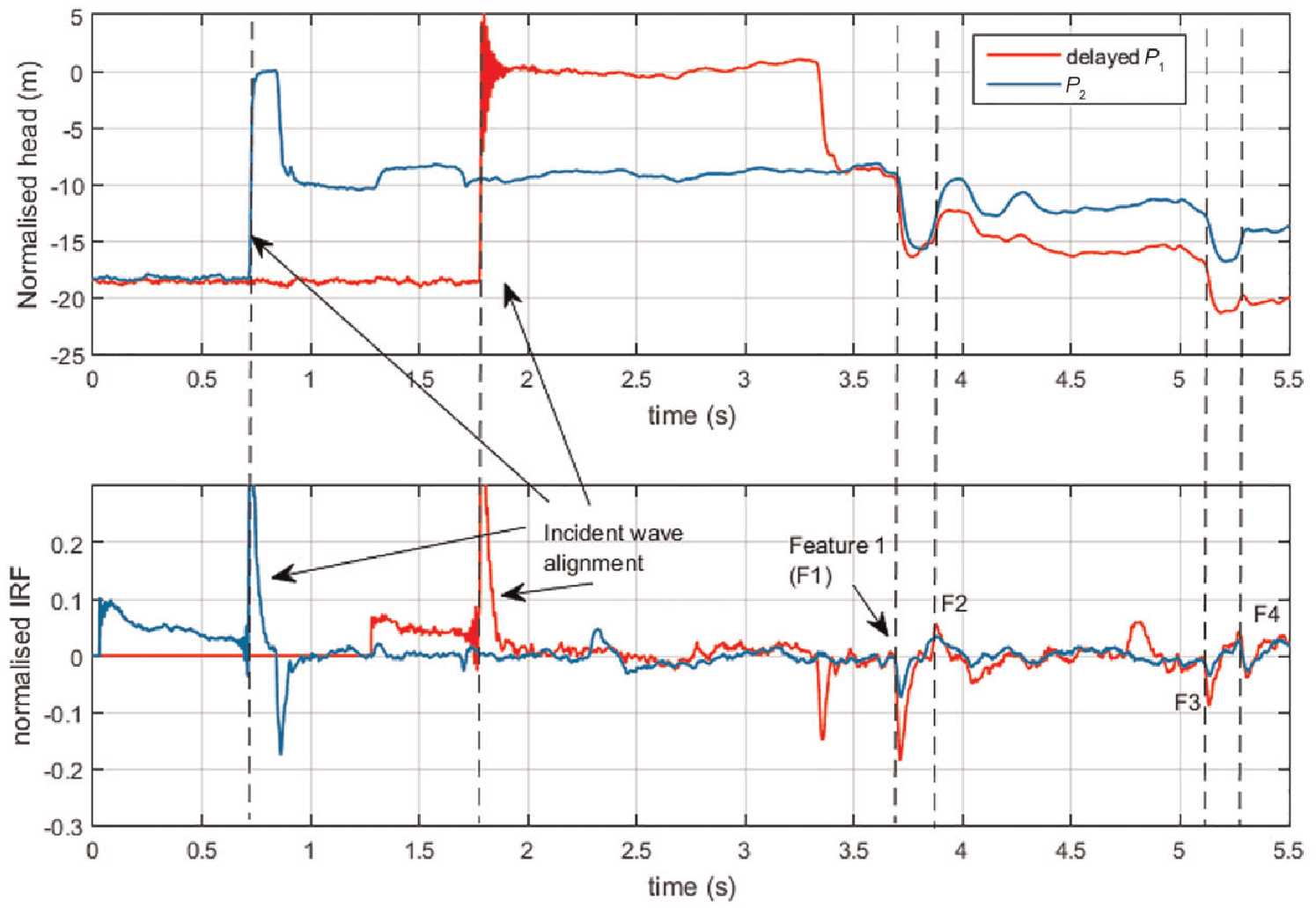
To examine the pipe section at the left side of M1, the transient pressure wave $P_{1}$ and the compositional IRF₁ were both delayed by $τ_{1} + τ_{2}$ . The delayed $P_{1}$ was compared with the original $P_{2}$ in Figure 9(a) and the delayed IRF₁ was compared with IRF₂ in Figure 9(b). It should be noted that the incident waves for both top and bottom subplots in Figure 9 are well aligned. The arrive time of the incident waves is 1.770 s on both the delayed $P_{1}$ trace and the delayed IRF₁ trace, and 0.738 s on both the delayed $P_{2}$ trace and the delayed IRF₂ trace. Apart from the aligned incident waves, good alignments can be also observed for feature 1 (F1) at (at 3.69 s), feature 2 (at 3.86 s), feature 3 (5.12 s) and feature 4 (5.26 s) in both subplots in Figure 9.

Figure 9.

(a) Delayed transient pressure wave $P_{1}$ versus original transient pressure wave $P_{2}$ and (b) delayed IRF₁ versus IRF₂.

The round-trip traveling time for the incident wave from M1 to the feature F1 is $T_{F 1} = 3.7 - 1.77 = 1.93$ (s). The corresponding distance to the M1 can be calculated by

L_{f} = \frac{a_{1} \cdot T_{F 1}}{2}

(18)

where $a_{1}$ is the wave speed in the 225AC pipe section and it is 1132 m/s based on the analyses in the former section. The distance is calculated as 1092 m, which corresponds to the pipe material and diameter change from 225AC to 300 DICL at chainage 865 m as shown in Figure 2. The actual distance recorded in Figure 2 is 1080 m (chainage 1945 − chainage 865 = 1080 m) and thus the relative error is 1.1%. The error is relatively small given that $\pm 20$ m uncertainties are involved in the measurement of the chainage using the GPS data. The reflection ratio r at this location is estimated as -20% from the IRF₁ trace and the theoretical value can be estimated by Equation (10) as −25.4%. The underestimation of the reflection ratio can be ascribed to the wave dissipation and dispersion in the pipe, which will diminish the spikes in the IRF trace.

The round-trip traveling time for the incident wave from the feature F1 to the feature F3 is $T_{F 2} = 5.12 - 3.7 = 1.42$ (s). By using Equation (18), the distance between these two features can be calculated as 848.5 m. Thus, the distance from feature F3 to M1 is estimated as 1940.5 m which corresponds to the T-junction at chainage 0 as shown in Figure 2. The actual distance recorded in Figure 2 is 1945 m which is very close to the estimated location with an error of 0.2%.

Apart from the aligned features F1 and F3, another two features F2 and F4 can be observed just following F1 and F3, respectively, with a same time delay of around 0.14 s. It can be also observed that the time delay is equal to the round-trip traveling time for the incident waves from M2 to another feature (labeled as F5) at the right side of pipe. Detailed analysis of the feature F5 will be given in the next section. Thus, these two features F2 and F4 can be explained as higher-order wave reflections with their traveling paths as PG–F1–F5–P2 and PG–F3–F5–P2, respectively.

The small section between chainage 911 and chainage 1002 corresponding to 225MSC section cannot be observed using IRFs since the change in impedance is not significant.

(b) Right side of M2

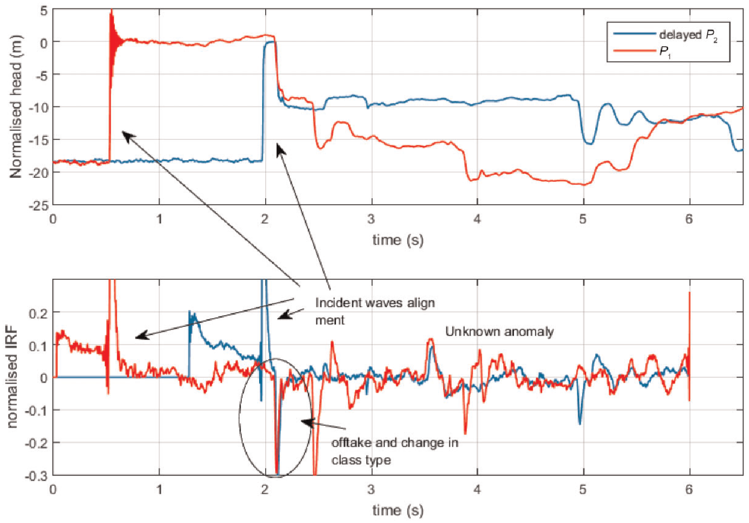
To examine the pipe section at the right side of M2, the transient pressure wave $P_{2}$ and the compositional IRF₂ were both delayed by $τ_{1} + τ_{2}$ . The delayed $P_{2}$ was compared with the original $P_{1}$ in Figure 10(a) and the delayed IRF₂ was compared with IRF₁ in Figure 10(b). The arrive time of the incident waves is 1.97 s on both the delayed $P_{2}$ trace and the delayed IRF₂ trace, and 0.53 s on both the delayed $P_{1}$ trace and the delayed IRF₁ trace. Good alignments can be also observed for feature 1 (F5) at 2.11 s in both subplots. A zoomed-in plot is given in Figure 11 for the spikes at 2.11 s.

Figure 10.

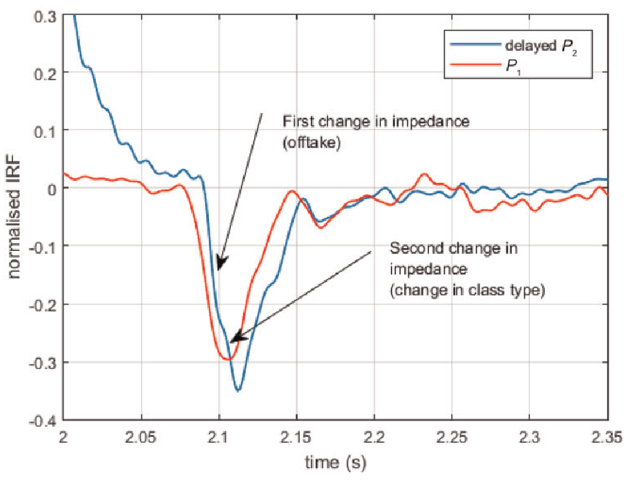
(a) Delayed transient pressure wave $P_{T 2}$ versus original transient pressure wave $P_{T 1}$ and (b) delayed IRF₂ versus IRF₁.

Figure 11.

Zoomed-in plots for the delayed IRF₂ and IRF₁.

The round-trip traveling time for the incident wave from M2 to the feature F5 is $T_{F 1} = 2.11 - 1.97 = 0.14$ (s). The corresponding distance to the M1 can be calculated as 80 m, which corresponds to the offtake at chainage 3433 m and change in class type at 3358 m as shown in Figure 2. These two pipe discontinuities are too close together and are difficult to be distinguished from each other.

Two virtual spikes can be found in the IRF traces without any distinctive pressure head changes. According to Equation (13), the time interval between the spike in $s R_{R}$ and the corresponding spike in $R_{R 2}$ is 2 $τ_{2}$ which is equal to the time interval between the matched spikes at 2.11 s and the spike at 3.55 s in IRF₁ trace. Thus, the virtual spike at 3.55 s is ascribed to feature F5 as well. Similar analysis can be conducted for IRF₂, and it can be found that the virtual spike at 3.55 s is ascribed to the feature F1 since the time interval between this spike with the one at 2.47 s is close to $2 τ_{1}$ . Due to the factor s in front of $R_{R}$ in Equation (7), the magnitude of the virtual spikes will be significantly reduced. Thus, only large impedance changes can induce virtual spikes and the virtual spikes induced by small impedance changes will be submerged in the noise.

Discussion

Comparing the transient-based technique and the hydroacoustic noise-based technique shows that both methods can effectively detect condition changes in this field pipeline. However, the hydroacoustic noise-based method does not require generating a sharp water hammer wave which is required for hydraulic transient-based method. This can save a large amount of time and effort in the field tests and makes field application more efficient, and less risky. Similar to hydraulic transient-based methods, the new method is cost-effective as a single test can inspect a long section of the pipeline, spanning several kilometers. It is also nondestructive, ensuring that the operation of the pipeline system remains unaffected. Note that the resolution of the hydroacoustic noise-based method is limited by strong wave attenuation in this large and long pipe. Future field experiments will demonstrate the high resolution achievable with the new method. However, the resolution that can be achieved using this hydroacoustic noise-based method is lower than some techniques, such as ultrasonic scanning.³ As another nondestructive method for pipe condition assessment, ultrasonic scanning can only assess a short section (e.g., 1 m) of the pipeline, and thus applying such a technique in a long transmission pipeline will be expensive and labor-intensive. Therefore, the new technique is suitable for long transmission pipelines for an initial scan. Other techniques such as the ultrasonic guided wave can be then applied to targeted pipe sections for a more refined assessment.

The hydroacoustic noise generation and propagation are closely related to the pipe diameter, pipe material, and internal pressure. The noise magnitude from a similar discharge decreases if the pipeline has a larger diameter, higher internal pressure, or is made of plastic materials. Stronger wave attenuation occurs in pipelines buried underground, resulting in smaller wave reflections from anomalies in the pipeline system. The signal-to-noise ratio, influenced by the magnitude of useful hydraulic waves and wave attenuation, impacts the technique's accuracy. Potential sources of interference include background water flow noise and the operation of hydraulic devices (e.g., pumps) in the pipeline systems. These can decrease the signal-to-noise ratio, reducing the quality of the IRF generated from the useful hydroacoustic noise.

Conclusion

A field study has been conducted on the condition assessment of a field water transmission pipeline using hydroacoustic noise generated by discharging water from a valve. The hydroacoustic noise collected at the standpipes is of much smaller magnitude, especially for the pressures at the measurement points. The field study shows that hydroacoustic noise can replace conventional hydraulic transient pressure waves of large magnitude for pipe condition assessment.

The hydroacoustic noise has a wide spectrum at the generation point but it dissipates significantly at the high frequency range. At the measurement points that are hundreds of meters away from the generation point, the energy of the hydroacoustic noise concentrates below 100 Hz. Resonance peaks can be found in the pressure spectrum due to the wave oscillation in the standpipe and thus shorter standpipes are recommended to increase the resonance frequencies of the standpipe.

A signal deconvolution process can transfer the measured hydroacoustic pressures to a compositional IRF which is composed of IRFs of different pipe sections. The mathematical equation of the compositional IRF can be used to interpret the spikes on the IRF traces. It shows the compositional IRF consists of the spikes corresponding to the incident wave, and wave reflections from both sides of the pipe. Some virtual spikes also exist in the IRF traces, and they are induced by large impedance changes. A time-shifting process on the compositional IRFs can be used to identify the direction of the wave reflection and thus localize the impedance changes.

Compared to the conventional transient-based techniques for pipe condition assessment, the proposed hydroacoustic technique in this paper inherits the merits of the transient-based techniques, such as the noninvasive and nondestructive properties, and the large detection coverage. It also overcomes some shortcomings of the transient-based techniques, such as large pipe vibration and low signal-to-noise ratio.

Footnotes

Declaration of conflicting interests

The author(s) declared no potential conflicts of interest with respect to the research, authorship, and/or publication of this article.

Funding

The author(s) disclosed receipt of the following financial support for the research, authorship, and/or publication of this article: The research presented in this paper has been supported by the Australian Research Council through the Linkage Project Grant LP210301373.

ORCID iDs

Wei Zeng

Martin Lambert

Data availability statement

The experimental data used during the study are available from the corresponding author by request.

References

Ceravolo

Civera

Lenticchia

, et al. Detection and localization of multiple damages through entropy in information theory. Appl Sci 2021; 11(13): 5773.

Yeung

. Time-domain spectral finite element method for analysis of torsional guided waves scattering and mode conversion by cracks in pipes. Mech Syst Signal Process 2019; 128: 305–317.

Zang

Z-D

, et al. Ultrasonic guided wave techniques and applications in pipeline defect detection: a review. Int J Pressure Vessels Pip 2023; 206: 105033.

Mostafapour

Davoudi

. Analysis of leakage in high pressure pipe using acoustic emission method. Appl Acoust 2013; 74(3): 335–342.

Che

T-C

Duan

H-F

Lee

P J

. Transient wave-based methods for anomaly detection in fluid pipes: a review. Mech Syst Signal Process 2021; 160: 107874.

Sanz

Pérez

Kapelan

, et al. Leak detection and localization through demand components calibration. J Water Resourc Plann Manage 2016; 142(2): 04015057.

Wang

Lin

Keramat

, et al. Matched-field processing for leak localization in a viscoelastic pipe: an experimental study. Mech Syst Signal Process 2019; 124(6): 459–478.

Pan

Duan

H-F

Meniconi

, et al. FRF-based transient wave analysis for the viscoelastic parameters identification and leak detection in water-filled plastic pipes. Mech Syst Signal Process 2021; 146: 107056.

Wong

Chiu

Kodikara

. Using distributed optical fibre sensor to enhance structural health monitoring of a pipeline subjected to hydraulic transient excitation. Struct Health Monit 2018; 17(2): 298–312.

10.

Al-tofan

Elkholy

Khilqa

, et al. Use of lower harmonics of pressure oscillations for blockage detection in liquid pipelines. J Hydraulic Eng 2019; 145(3): 04018090.

11.

Meniconi

Brunone

Ferrante

, et al. Transient hydrodynamics of in-line valves in viscoelastic pressurized pipes: long-period analysis. Exp Fluids 2012; 53(1): 265–275.

12.

Louati

Ghidaoui

. Eigenfrequency shift mechanism due to an interior blockage in a pipe. J Hydraulic Eng 2018; 144(1): 04017055.

13.

Duan

. Sensitivity analysis of a transient-based frequency domain method for extended blockage detection in water pipeline systems. J Water Resour Plann Manage 2016; 142(4): 04015073.

14.

Zeng

Gong

Lambert

, et al. Detection of extended blockages in pressurised pipelines using hydraulic transients with a layer-peeling method. In: IOP Conference Series: Earth and Environmental Science, Vol. 240, no. 5. Institute of Physics Publishing, 2019.

15.

Jing

Wang

, et al. An approximate inverse scattering technique for reconstructing blockage profiles in water pipelines using acoustic transients. J Acoust Soc Am 2018; 143(5): EL322–EL327.

16.

Blasten

Zouari

Louati

, et al. Blockage detection in networks: the area reconstruction method. Math Eng 2019; 1(4): 849–880.

17.

Zeng

Gong

Zecchin

, et al. Condition assessment of water pipelines using a modified layer-peeling method. J Hydraulic Eng 2018; 144(12): 04018076.

18.

Gong

Simpson

Lambert

, et al. Detection of distributed deterioration in single pipes using transient reflections. J Pipeline Syst Eng Practice 2013; 4(1): 32–40.

19.

Misiunas

. Failure monitoring and asset condition assessment in water supply systems. Lund, Sweden: Lund University, 2005.

20.

Stephens

Lambert

Simpson

. Determining the internal wall condition of a water pipeline in the field using an inverse transient model. J Hydraulic Eng 2013; 139(3): 310–324.

21.

Gong

Lambert

Zecchin

, et al. Field study on non-invasive and non-destructive condition assessment for asbestos cement pipelines by time-domain fluid transient analysis. Struct Health Monit 2016; 15(1): 113–124.

22.

Shucksmith

Boxall

Staszewski

, et al. Onsite leak location in a pipe network by cepstrum analysis of pressure transients. J AWWA 2012; 104(8): E457–E465.

23.

Gong

Lambert

Nguyen

STN

, et al. Detecting thinner-walled pipe sections using a spark transient pressure wave generator. J Hydraulic Eng 2018; 144(2): 06017027.

24.

Meniconi

Brunone

Ferrante

, et al. Anomaly pre-localization in distribution–transmission mains by pump trip: preliminary field tests in the Milan pipe system. J Hydroinf 2015; 17(3): 377–389.

25.

Ghazali

Beck

SBM

Shucksmith

, et al. Comparative study of instantaneous frequency based methods for leak detection in pipeline networks. Mech Syst Signal Process 2012; 29(5): 187–200.

26.

Tijsseling

Lambert

Simpson

, et al. Wave front dispersion due to fluid-structure interaction in long liquid-filled pipelines. In: 23rd IAHR Symposium. Yokohama, Japan. 2006.

27.

Zanganeh

Jabbari

Tijsseling

, et al. Fluid-structure interaction in transient-based extended defect detection of pipe walls. J Hydraulic Eng 2020; 146(4): 04020015.

28.

Zeng

Cazzolato

Lambert

, et al. Coherenceogram for leak detection in water pipes. J Sound Vibr 2022; 530: 116979.

29.

Zeng

Gong

Simpson

, et al. Paired-IRF method for detecting leaks in pipe networks. J Water Resour Plann Manage 2020; 146(5): 04020021.

30.

Zeng

Zecchin

Cazzolato

, et al. Extremely sensitive anomaly detection in pipe networks using a higher-order paired-impulse response function with a correlator. J Water Resour Plann Manage 2021; 147(10): 04021068.

31.

Nguyen

STN

Gong

Lambert

, et al. Least squares deconvolution for leak detection with a pseudo random binary sequence excitation. Mech Syst Signal Process 2018; 99(1): 846–858.

32.

Zeng

Lambert

Gong

, et al. Anomaly detection in targeted pipe sections in water pipe systems using hydroacoustic signal deconvolution. J Hydraulic Eng 2024; 150(1): 04023059.

33.

Gong

Stephens

Arbon

, et al. On-site non-invasive condition assessment for cement mortar-lined metallic pipelines by time-domain fluid transient analysis. Struct Health Monit 2015; 14(5): 426–438.

Field study on proactive pipe condition assessment using hydroacoustic noise

Abstract

Keywords

Introduction

Compositional impulse response function

Pressure deconvolution

Time-shifting the IRFs to overlap anomaly-induced spikes

Field pipe system and tests

Data analyses

Signal filter

Signal deconvolution

Time-shifting the IRFs to overlap anomaly-induced spikes

Discussion

Conclusion

Footnotes

Declaration of conflicting interests

Funding

ORCID iDs

Data availability statement

References