
Abstract
This paper investigates nonlinear guided wave propagation in square tubes with material nonlinearity for the first time. The dispersion characteristics of guided waves in a square aluminum tube are first analyzed and presented. A pair of longitudinal wave modes is selected as fundamental waves and second harmonics. The selected mode pair is identified to meet the internal resonance condition. Then, a three-dimensional finite element model is developed to simulate the second harmonic generation and propagation in the square tube. When the fundamental waves propagate in the square tube, the second harmonics are generated due to the self-interaction of the fundamental waves and inherent material nonlinearity. The generated second harmonics are manifested to be cumulative with the almost linearly increased nonlinear acoustic parameter versus propagation distance. Subsequently, the experiment is carried out to confirm the simulated results and they are considerably consistent. Finally, the generated second harmonics are employed to evaluate different levels of thermal fatigue damage, which is introduced into the square tube by applying increasing thermal cycles. The nonlinear acoustic parameter increases with the growing thermal cycles, which indicates the induced second harmonics are sensitive to thermal fatigue damage. The findings of this study provide insights into practical applications for the detection and evaluation of early-stage damage in square tubes using second harmonic generation of longitudinal waves.
Keywords
Introduction
Square tubes are a kind of tubular structures that have wide applications in engineering. Compared with circular pipes, which are often adopted in pipeline systems, 1 square tube functions as structural elements in buildings and machines due to their superior bending strength. 2 There are many factors, for example, impact, corrosion, cyclic load, and temperature variation that could contribute to damage generation and further accumulation. Therefore, it is considerably important to conduct the damage diagnosis and inspection. Otherwise, the incipient damage without manual intervention or professional maintenance may eventually result in catastrophic consequences, such as huge economic loss and even the loss of life.
In the past decades, numerous techniques concerning nondestructive testing (NDT) and structural health monitoring (SHM) were proposed and proven to be efficient and effective in the detection of different kinds of damage in various structures.3–7 Among those proposed approaches, guided wave techniques possess distinct advantages over other techniques,8,9 due to the long distance inspection capacity and high sensitivity to different kinds of defects. 10 Particularly, the nonlinear guided wave techniques like second harmonic generation and guided wave mixing are quite attractive because of their capacity to detect the changes in material microstructure and early-stage damage. 11 Many studies were reported regarding damage detection in tubular structures with material nonlinearity using nonlinear guided wave techniques. For example, Li and Cho 12 selected a high-frequency longitudinal wave mode to generate the second harmonics in the metal tube and assessed different severity of thermal fatigue damage with the nonlinear guided waves. Yeung and Ng 13 investigated the mixing of non-dispersive torsional mode with two different frequencies in the aluminum pipe to generate the combinational harmonics and further quantified the fatigue damage. A combinational harmonic at difference frequency with backward propagation ability could be induced by mixing two different longitudinal modes in circular pipes, and its sensitivity to degradation in a local area was examined. 14 Jiang et al. 15 evaluated the thermal fatigue damage in the carbon fiber-reinforced composite pipe with nonlinear guided waves. However, these studies in tubular structures using nonlinear guided wave techniques were only confined to circular pipes. In the literature, little research investigates the nonlinear guided waves in square tubes with material nonlinearity. Wan et al. 16 first studied the feasibility of using linear guided wave technique to inspect circular hole as well as slot on the tube surface. In this literature, the dispersion characteristics of the square tube are first presented. Compared with the dispersion relations of the circular tube, the dispersion characteristics of the square tube are much more complicated, which makes it quite difficult and challenging for the investigation of nonlinear guided waves, for example, the wave mode selection and analysis of internal resonance condition. However, to guarantee the safety, integrality and functionality for machines and buildings, NDT and SHM for square tubes to detect incipient damage with nonlinear guided wave technique are of increasing urgency and significance. To this end, this paper presents a comprehensive study to theoretically, numerically, and experimentally investigate second harmonic generation in isotropic square tubes with material nonlinearity. The first concern is whether there is appropriate wave mode pair that could be found in dispersion curves to satisfy the internal resonance condition for second harmonic generation in square tubes. The second focus is how to excite and measure those guided wave modes with feasible piezoelectric transducer (PZT) configurations for square tubes in practice.
The article is organized as follows. Firstly, the nonlinear elasticity theory for the waveguide with arbitrary cross-section and semianalytical finite element (SAFE) method for analyzing dispersion characteristics is reviewed. Then, the dispersion curves of a given aluminum square tube are analyzed and presented, based on which a mode pair is selected as fundamental waves and second harmonics. This selected mode pair is proven to satisfy the internal resonance condition. Subsequently, a three-dimensional (3D) finite element (FE) model is built to gain physical insight into nonlinear guided wave generation and propagation in the square tube with material nonlinearity. Next, the experiment is carried out with proposed PZT configurations to validate the simulated results. After that, the thermal fatigue damage is introduced into the square tube by applying thermal cycles. The thermal fatigue level can be correlated with experimentally generated second harmonics using the nonlinear acoustic parameter. The final section draws the conclusions.
Theoretical foundation
Nonlinear elasticity theory for wave propagation
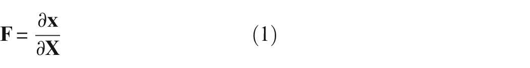
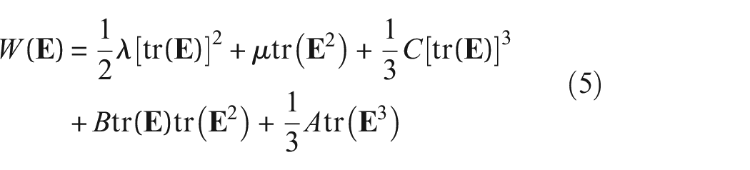
The nonlinear elasticity theory for wave motion based on finite deformation theory and material nonlinearity are briefly reviewed.17,18 In order to analyze the motion of a continuous medium and describe its deformation, two different coordinate systems are introduced. One is in the initial configuration, the other is in the current configuration of the medium as shown in Figure 1.
where

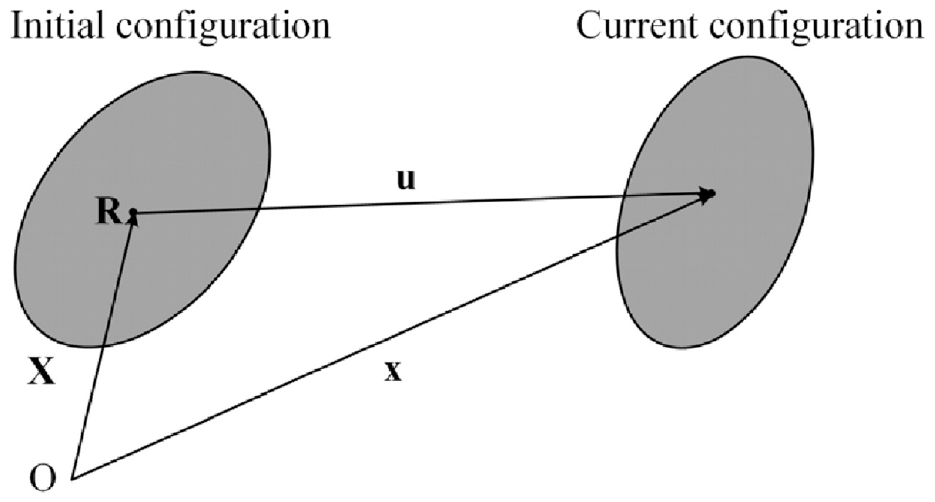
Deformation description with Lagrangian coordinates in the initial configuration and Eulerian coordinates in the current configuration.
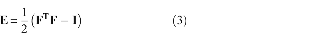
The Green-Lagrangian strain tensor
or
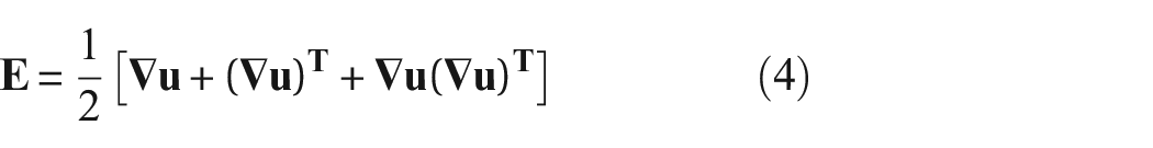
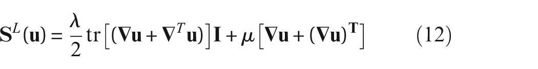
where T is the transposition of the matrix;
where
The momentum equation for homogeneous isotopic medium is written as 20
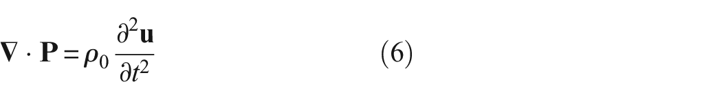
where
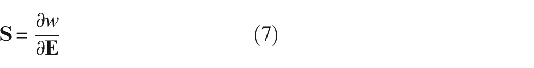
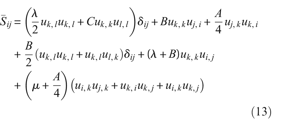
The

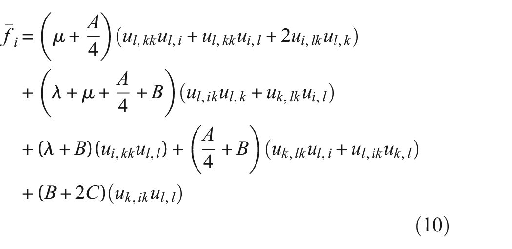
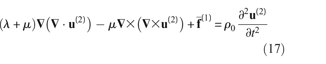
Substituting Equations (4), (5), (7), and (8) into Equation (6) and simplification, the governing equation for the motion in the homogeneous isotropic medium can be formulated as
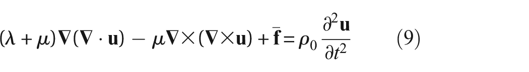
where
where

where
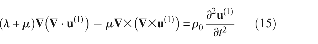
The nonlinear boundary value problem associated with Equations (9) and (11) can be solved based on the perturbation method.
17
The displacement field

where

where

where
The guided waves in the waveguide are assumed to propagate along the z direction, as shown in Figure 2. The fundamental wave field can be expressed as

where
where
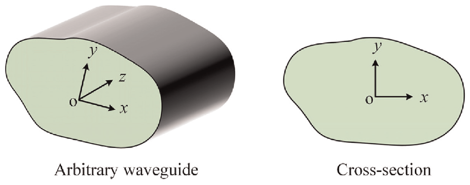
Schematic illustration of an arbitrary waveguide with reference coordinate system.
Here,
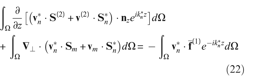
The divergence theorem is applied to the second term in Equation (22), and one can obtain
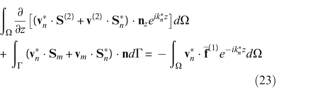
where
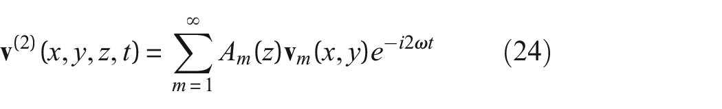
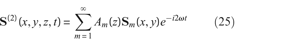
where
Substituting Equations (24) and (25) into Equation (23), a set of ordinary differential equations can be obtained based on the orthogonality relation 22
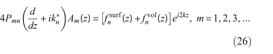
where
Here,

where
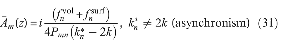
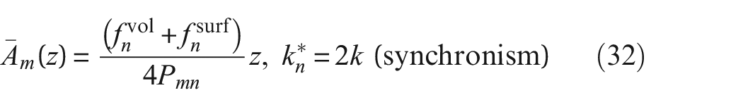
According to Equation (32), it is obvious that the modal amplitude concerning the secondary mode grows with propagation distance z when synchronism or phase velocity matching
SAFE method
For an arbitrary waveguide, as shown in Figure 2, the SAFE method utilizes an analytical solution in the propagation direction. The FE approximation is implemented in the cross-section for the waveguide. There are two implementation approaches for the SAFE method. The first implementation approach is based on FE programming in MATLAB. 23 This requires the researcher proficient in FE code, which is quite challenging for the researchers who are not familiar with FE code. To overcome this drawback, the group of Dr. Liu developed and released an open-source tool called semi-analytical finite element dispersion calculator (SAFEDC), which is based on the SAFE method to calculate the dispersion characteristics. 24 The general section module in SAFEDC enables the researcher to calculate and obtain the dispersion relations for the waveguide with arbitrary cross-section easily. After importing the cross-section file, meshing, and defining material properties, the SAFEDC will call MATLAB to run the calculation.
The second implementation approach is based on the partial differential equation (PDE) module in the commercial software COMSOL.14,25,26 The key to this method is to derive the correct PDE coefficients for the question of interest. The PED coefficient is deduced by comparing the governing equation for the problem of interest with the general expression of the eigenvalue equation in the COMSOL PDE module. After building the cross-section of the waveguide, inputting correct PDE coefficients, and then meshing, the eigenvalue equation will be solved by the parametric sweep of the given wavenumber k or angular frequency
Nonlinear SAFE algorithm
To analyze the internal resonance condition for complex waveguides, the nonlinear SAFE algorithm is proposed, which is based on COMSOL and MATLAB.
27
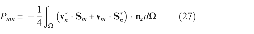
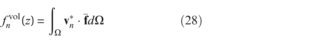
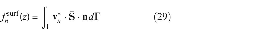
The nonlinear SAFE algorithm can be implemented in three steps. Firstly, the dispersion characteristics of the complex waveguide are solved in COMSOL PDE module. Secondly, by the powerful postprocessing of COMSOL, the stress tensor, velocity vector, and their corresponding complex conjugates, as well as the nonlinear terms in Equations (27) to (29), are computed in the area and boundary of the cross-section for the waveguide. Thirdly, with the data extracted from COMSOL, the integral in Equations (27) to (29) and the modal amplitude for secondary mode in Equation (32) are calculated in MATLAB. If there is power flux transferring from the fundamental wave field to the secondary wave field, the modal amplitude
Dispersion analysis and wave mode selection
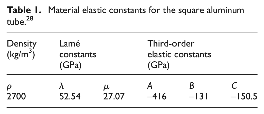
Considering a square aluminum tube, as shown in Figure 3, the length of the side for the outer square is 25 mm. The wall thickness of the square tube is 1.6 mm. The length of the square tube is 2000 mm. The material elastic constants for the tube are given in Table 1. With the sizes and material elastic constants for the square tube, the dispersion curves calculated by SAFEDC are plotted in Figure 4. It can be easily seen that the dispersion characteristics of the square tube are rather complex. For simplicity, the guided wave modes are designated as labels (M1, M2, …, M25, …, M40…) according to their appearance sequence. Meanwhile, the dispersion curves of a circular aluminum tube with an outer diameter of 25 mm and thickness of 1.6 mm are given in Figure 5. Compared with dispersion relations of the circular tube. It is clear that the dispersion characteristics of the square tube are much more complex, which makes it difficult to analyze the guided wave propagation in square tubes and apply nonlinear guided wave techniques on square tubes.
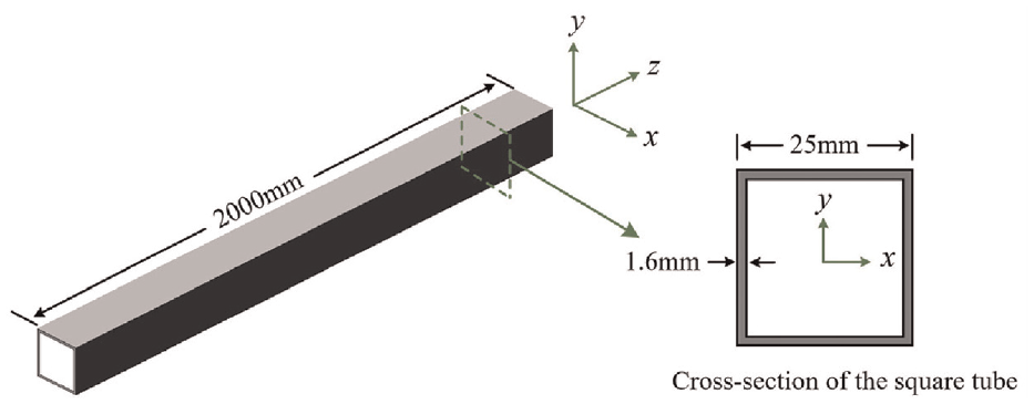
Schematic diagram of the square tube with dimensions.
Material elastic constants for the square aluminum tube. 28
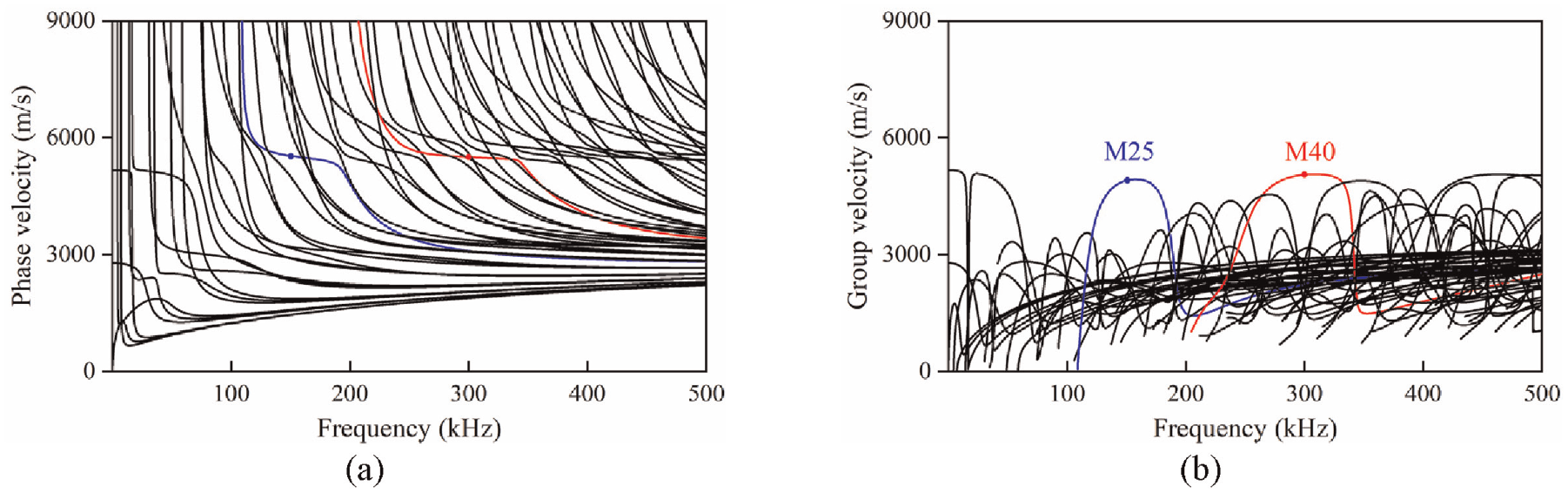
Dispersion curves for the square aluminum tube: (a) phase velocity and (b) group velocity.
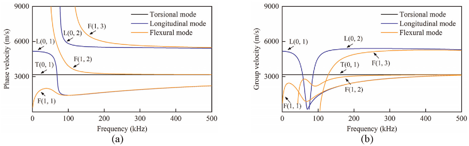
Dispersion curves for the circular aluminum tube: (a) phase velocity and (b) group velocity.
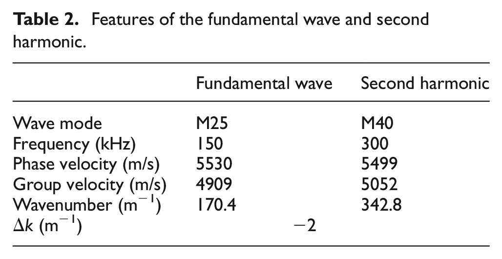
After analyzing the dispersion curves of the square tube, a pair of wave modes is selected, as shown in Figure 4, which are M25 mode at 150 kHz (blue line) for fundamental waves and M40 mode at 300 kHz (red line) for second harmonics. The corresponding phase velocity, group velocity, and wavenumber are summarized in Table 2. In the table,
Features of the fundamental wave and second harmonic.
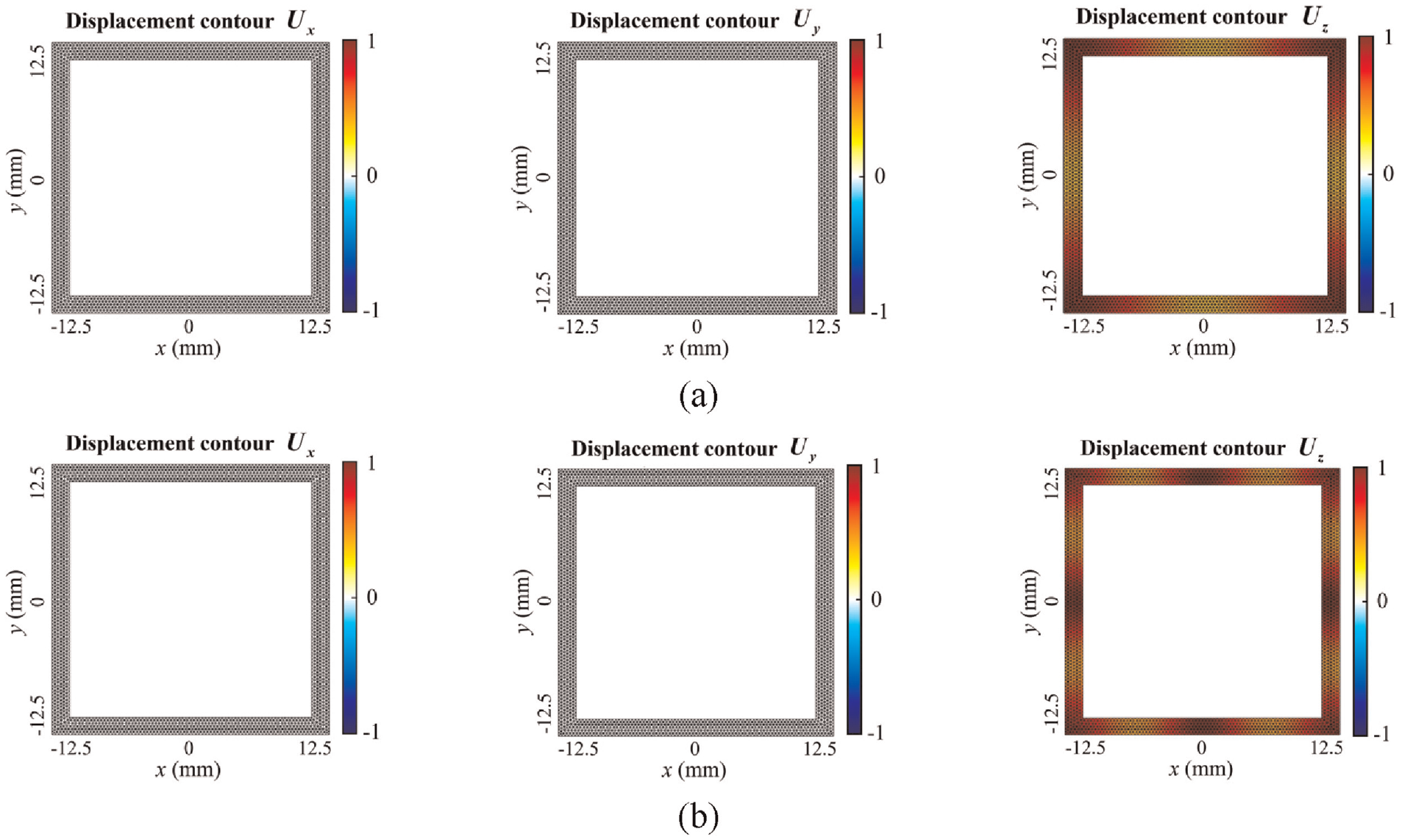
Mode shapes for fundamental waves and second harmonics: (a) M25 mode at 150 kHz and (b) M40 mode at 300 kHz.
As pointed out before, the internal resonance, which is essential for the generation of cumulative second harmonics, depends on two conditions: (1) synchronism or phase velocity matching; (2) nonzero power flux transferring from the fundamental wave field to the secondary wave field. According to the data given in Table 2,
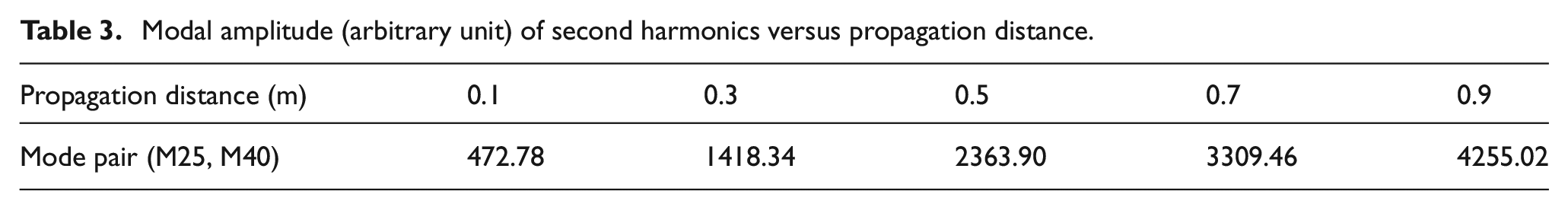
The eigenvalues relating to the dispersion characteristics of the square tube are first solved with COMSOL. Here, the eigenvalues computed by COMSOL for M25 and M40 modes are compared with the results calculated by SAFEDC, as shown in Figure 7. A good agreement can be found between SAFEDC and COMSOL, which demonstrates the validity and accuracy of both methods. Then, the modal amplitude regarding second harmonics for the selected mode pair (M25, M40) is calculated and listed in Table 3. It is evident that the modal amplitude of second harmonics grows with respect to propagation distance, which proves the selected mode pair satisfies the internal resonance condition.
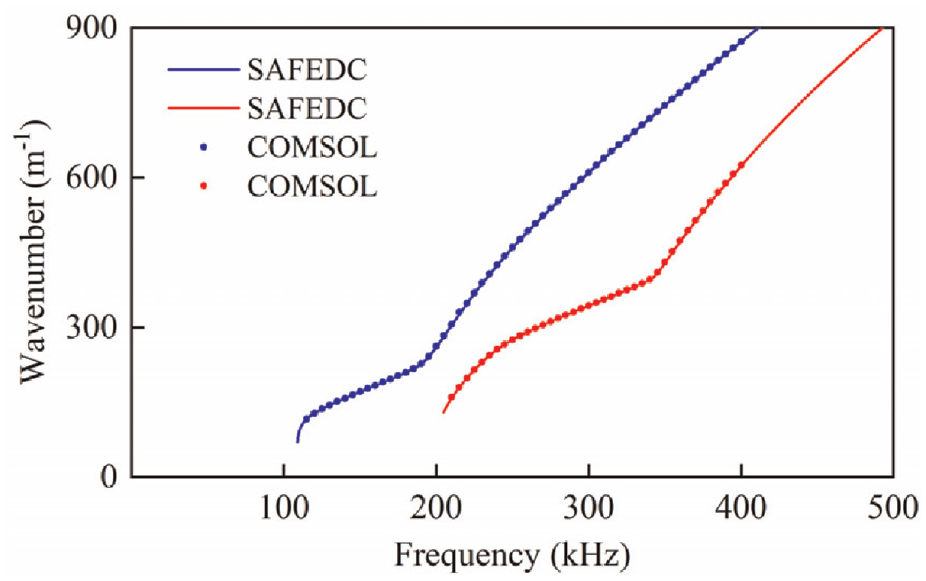
Comparison of eigenvalues between SAFEDC and COMSOL.
Modal amplitude (arbitrary unit) of second harmonics versus propagation distance.
FE simulation
FE model
In this section, a 3D FE model is developed to simulate second harmonic generation and propagation in the square tube using ABAQUS/Explicit. An 18-cycle Hanning-windowed tone burst signal is generated. The center frequency of the signal is 150 kHz. This excitation signal is applied as the displacement excitation at the end of the FE model, as shown in Figure 8. The direction of excitation is along the axial direction. The peak amplitude for the displacement excitation in the simulation is
where
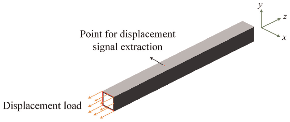
Schematic diagram of the 3D FE model.
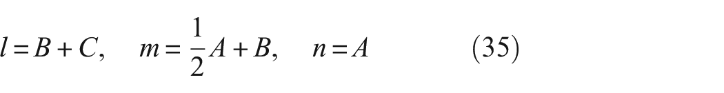
Then, the material nonlinearity for the FE model is implemented by a user-defined subroutine using VUMAT. In ABAQUS, the Murnaghan model is used to describe the strain energy function for material in the time domain FE model, which is expressed as 30
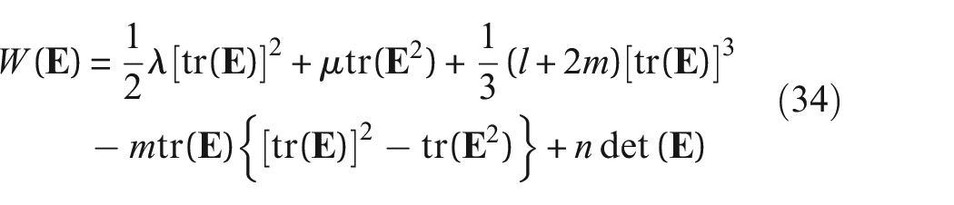
where l, m, and n are the Murnaghan constants. The Murnaghan model is actually equivalent to the Landau-Lifshiz hyperelastic constitutive model in Equation (5), and the transformation relationship between Murnaghan constants and the third-order elastic constants is given by 31
In order to achieve calculation stability and adequate accuracy, the element size (
Simulation results
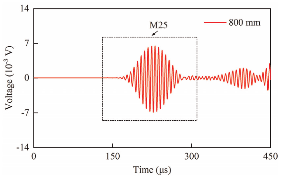
The axial displacement signal for a point, as shown in Figure 9 on the outer surface of the square tube, is plotted in Figure 9. The point is 800 mm far from the excitation position. Since the M25 mode at 150 kHz has the fastest group velocity among other wave modes, as shown in Figure 4(b), the first wave package in the dash window should be M25 mode. Meanwhile, it is noted that the group velocity of the second harmonics (5052 m/s) is very close to that of the fundamental waves (4909 m/s), as presented in Table 2. As a result, when the fundamental waves propagate along the axial direction in the tube, the generated second harmonics can travel with the wave package of fundamental waves and then separate from the other wave modes after a certain propagation distance. Therefore, the simulated axial displacement signal in the dash window, as shown in Figure 9, is intercepted and reserved for analysis. The signal out of the dash window is adjusted to be zero. The beginning and end of the dash window are from 130 to 310 µs with a duration of 180 µs. This signal processing method is also used to handle the received signal in the experiment.
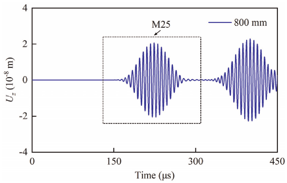
The time domain axial displacement signal under the propagation distance of 800 mm.
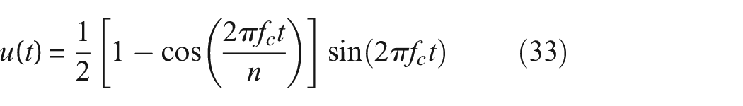
Figure 10(a) presents the intercepted axial displacement signal after normalization, and the corresponding frequency domain is plotted in Figure 10(b). It is found that both quasi-static components and second harmonics are induced by the propagation of fundamental waves. However, the frequency range of the main lobe regarding the quasi-static components is very close to zero frequency, which makes it difficult to measure in the experiment. Therefore, the generated second harmonics become the focus of the present study. The nonlinear acoustic parameter is defined as follows 33
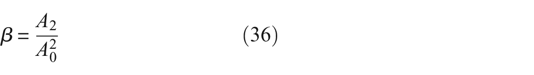
where
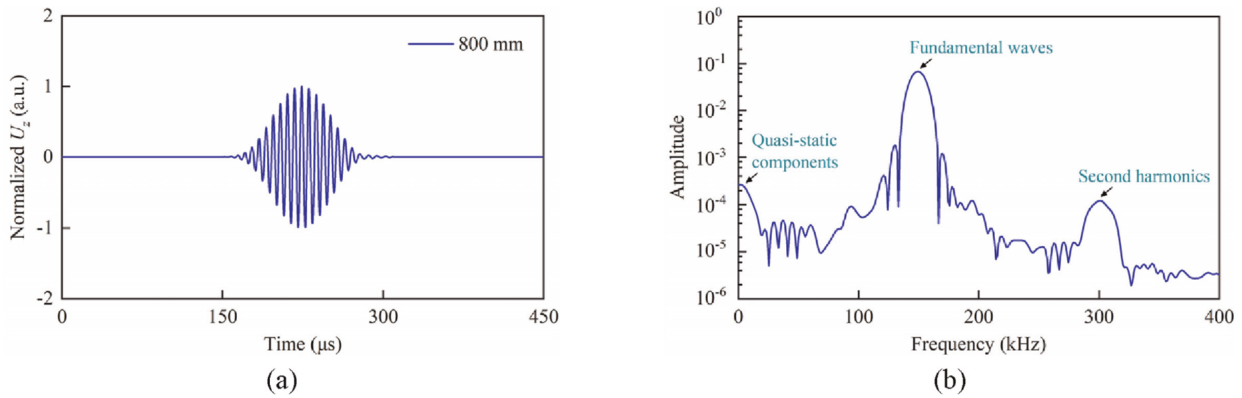
The axial displacement signal after processing: (a) time domain and (b) frequency domain.
The wave mode of fundamental waves and second harmonics are verified by transforming the received signals into a wavenumber-frequency spectrum by two-dimensional discrete fast Fourier transformation. 34 Sixty points with 1 mm for adjacent points are created in the FE model. The distance between the first point and the excitation position is 800 mm. The axial displacement signals at all measurement points are collected and transformed into a wavenumber-frequency contour, as shown in Figure 11. For the mode identification, the dispersion curves are also plotted in Figure 10. It is confirmed that the generated fundamental guided wave mode is M25 mode.
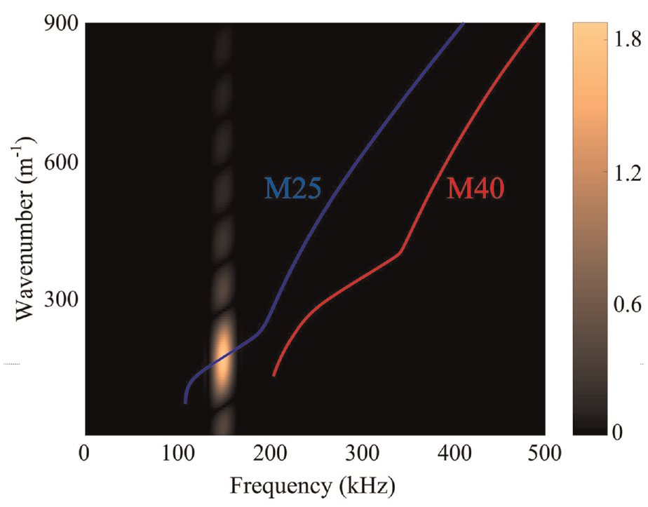
Wavenumber-frequency domain analysis for fundamental waves at 150 kHz.
Due to the fact that the amplitude of second harmonics is very small compared with that of fundamental waves, an approach called phase reversal is implemented to extract the time domain waveform of second harmonics from the wave package of fundamental waves. 35 The flowchart for the extraction of second harmonics is given in Figure 12. By superimposing the original and phase-reversed signal, the fundamental waves are counteracted, and the nonlinear guided waves, including second harmonics and quasistatic components, are obtained. Then, a high-pass filter with a cutoff frequency of 200 kHz is employed to filter the quasi-static components, and the time domain waveform of second harmonics is obtained. The wavenumber-frequency spectrum, as shown in Figure 13, indicates that the wave mode of the generated second harmonics is M40 mode, which is consistent with the theoretical analysis.
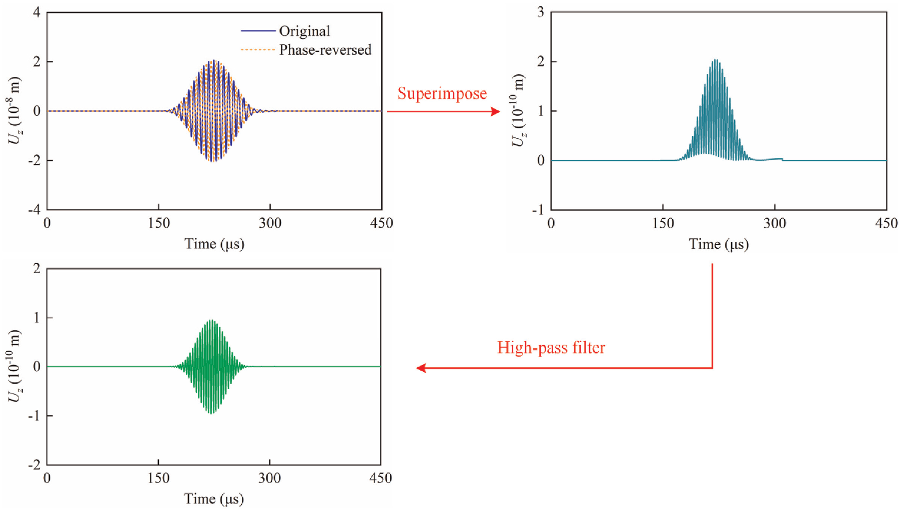
Flowchart for extracting time domain waveform of second harmonics from the wave package of fundamental waves.
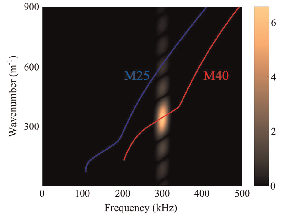
Wavenumber-frequency domain analysis for second harmonics at 300 kHz.
In addition, the cumulative effect versus propagation distance is also presented. Figure 14 shows an example of calculating the nonlinear acoustic parameter under different propagation distances. The calculation of nonlinear acoustic parameter uses the axial displacement signal at 800 mm as a baseline. The axial displacement signal at 1100 mm is first extracted. Then, by comparing with the axial displacement signal at 800 mm, the time delay (60.94 µs) for the wave package of fundamental waves at two different locations is obtained by cross-correlation. The dash window will move backward with the calculated time delay and is determined for the axial displacement signal at 1100 mm. The axial displacement at 1100 mm in the dash window is intercepted and transformed to the frequency domain to calculate the nonlinear acoustic parameter.
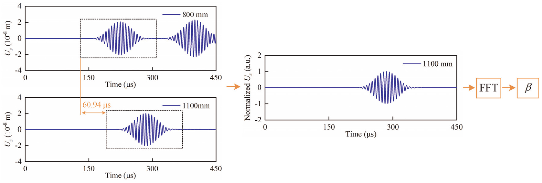
The flowchart for calculating the nonlinear acoustic parameter at different locations.
Figure 15 shows the nonlinear acoustic parameter versus propagation distance. The almost linearly increased nonlinear acoustic parameter indicates the generated second harmonics are cumulative. Thus, it is convinced that the selected mode pair satisfies the internal resonance condition. Besides, the group velocity of fundamental waves is calculated to be 4923 m/s, which is very close to the theoretic value (4909 m/s) in Table 2. This confirms the wave mode of the first wave package is M25 mode again.
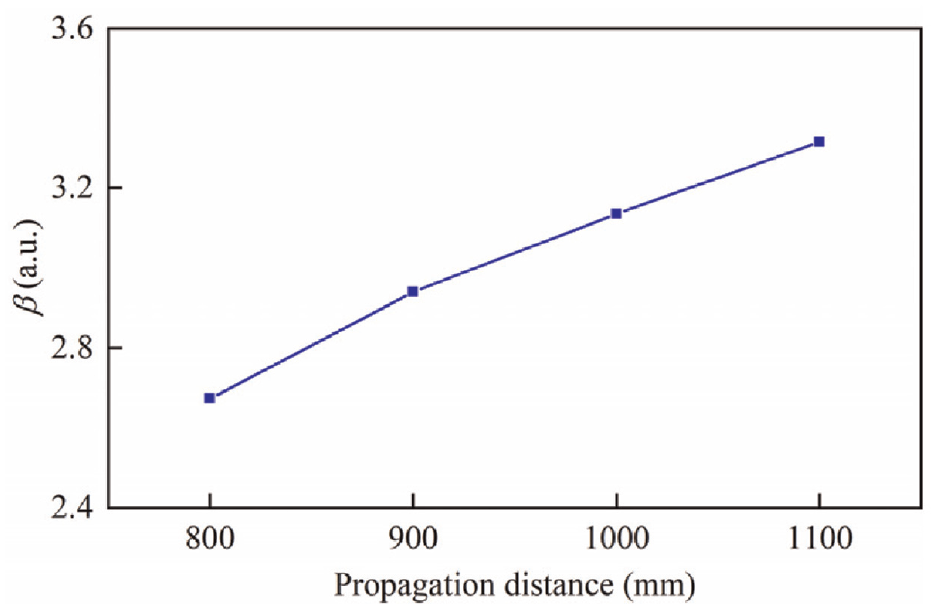
Nonlinear acoustic parameter versus propagation distance.
Experimental verification
Experimental setup
In this section, the ultrasonic measurements are conducted on a square aluminum tube, of which the material properties and dimensions are identical to FE model. The experimental setup for the ultrasonic measurements is shown in Figure 16. Firstly, the same excitation signal used in simulation is sent to the signal generator NI PXI-5412 by computer. After the signal is generated by signal generator, it is transmitted to the Ciprian high-voltage power amplifier. Subsequently, the signal is fed into the shear PZTs (Type Pz27, Ferroperm™ Piezoceramics, CTS Corporation, Kvistgård, Denmark) to excite the guided waves propagating the square tube.
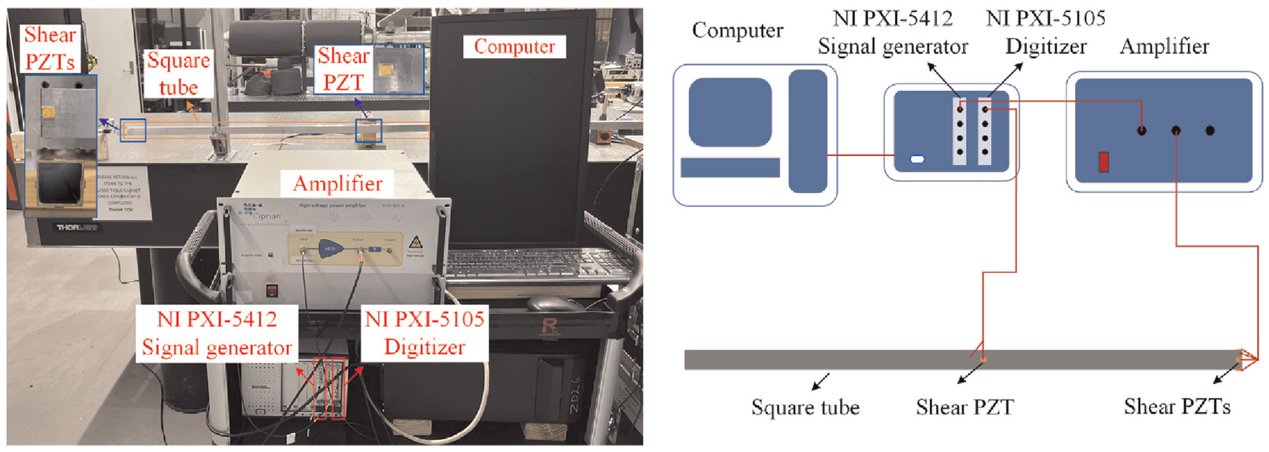
Experimental setup for ultrasonic measurements.
Here, using the conductive epoxy, four shear PZTs are bonded on the outer surface of the square tube close to the end with their length along the axial direction, as shown in Figure 17(a). The dimensions of the shear PZT are 6 mm in length, 5 mm in width, and 0.7 mm in thickness. The polarization direction of the shear PZT is parallel to the length direction. When the shear PZTs received the electric signals, it deforms in length direction as shown in Figure 17(b). Then, external forces produced by shear PZTs pull and push the tube end to generate the longitudinal waves. The generated longitudinal waves propagate in the square tube and are measured by one shear PZT bonded on the external surface of the tube 800 mm away from excitation PZTs as shown in Figure 15. The measured signal is received by the digitizer NI PXI-5105 and saved for further analysis. The signal is averaged 500 times to improve the signal-to-ratio.
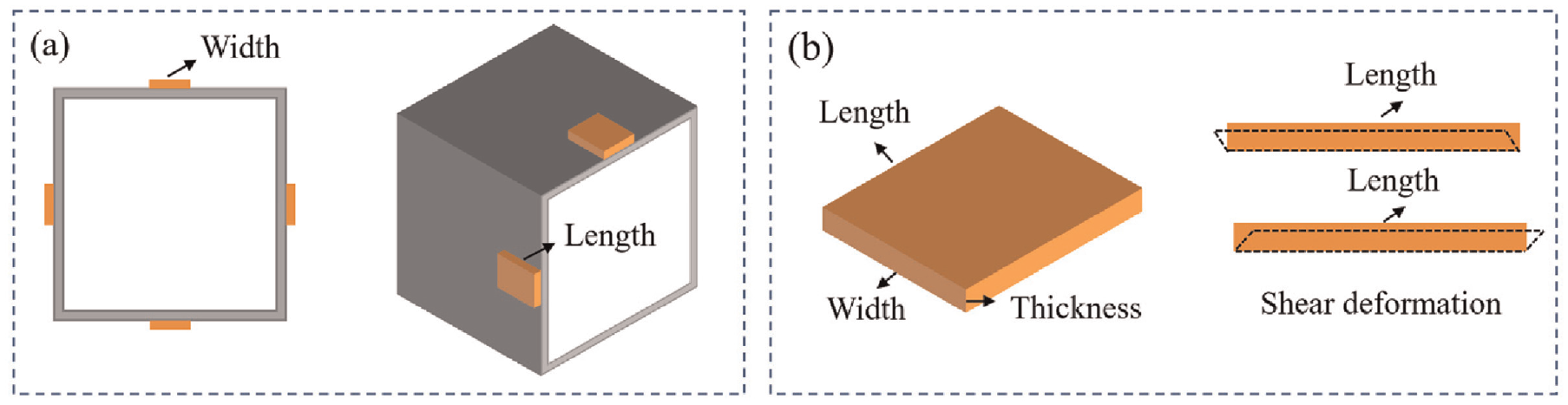
Schematic diagram about (a) shear PZT installation and (b) its deformation.
Experimental results
As aforementioned, the second harmonics is the concern in this research. Hence, the experimentally received signal is processed with a low-pass filter whose cutoff frequency is 400 kHz, through which other higher harmonics and high-frequency noises can be excluded. Figure 18 shows the experimentally measured signal after the low-pass filter. The first wave package in the dash window is intercepted and extracted for analysis. The beginning, end, and duration of the dash window are identical to that used in the simulation in Figure 9. After normalization, the experimental results are compared with the numerical ones in Figure 19. A good agreement can be found for fundamental waves between simulation and experiment. With four shear PZTs, the fundamental waves are well excited in the experiment. Then, the intercepted experimental signal after normalization is transformed to the frequency domain, and the corresponding frequency spectrum is plotted in Figure 20, in which the second harmonics are clearly observed.
Experimentally measured signal under a propagation distance of 800 mm.
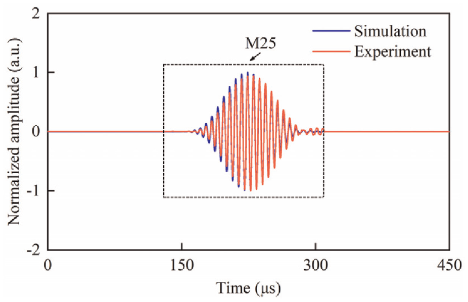
Comparison of time domain signals between simulation and experiment.
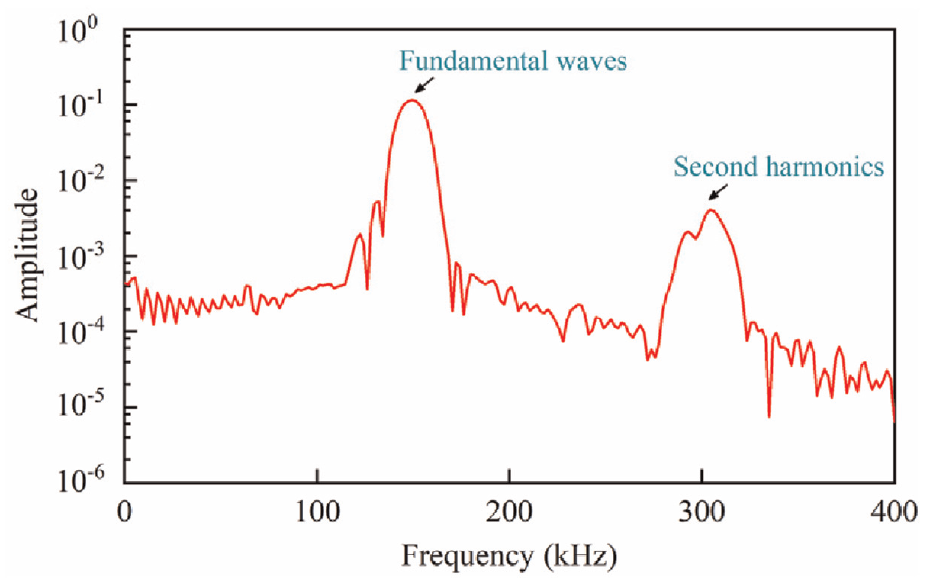
Frequency spectrum of the intercepted experimentally measured signal.
In addition, the cumulative effect versus propagation distance is also presented. Another three shear PZTs are bonded on the external surface of the tube at locations 900, 1000, and 1100 mm, respectively. Four times of ultrasonic measurements at each location are performed. The experimental nonlinear acoustic parameter versus propagation distance is plotted in Figure 21. It can be observed that the nonlinear acoustic parameter grows with the increase of propagation distance, which indicates the generated second harmonics are cumulative. Previous studies point out the instrument nonlinearity can also contribute to the second harmonic generation.13,36 To suppress the effect of the instrument nonlinearity, the measurement on the intact square tube is used as the baseline in the following investigation of damage assessment.
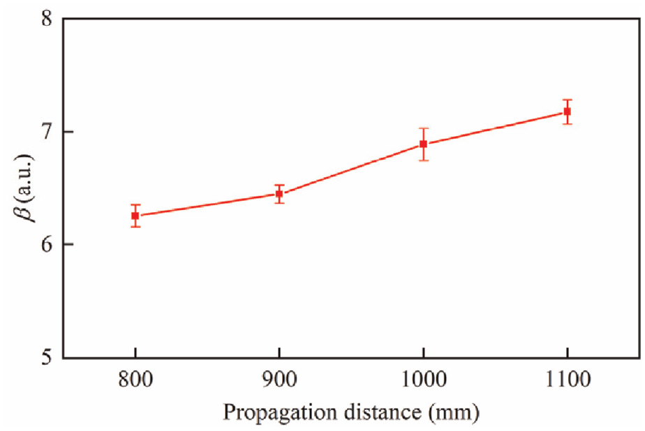
Experimentally measured nonlinear acoustic parameter versus propagation distance.
Damage assessment
In this section, the sensitivity of experimentally measured second harmonics to damage is examined. The generated second harmonics are utilized to assess thermal fatigue damage in the square tube. Thermal fatigue is one type of in-service damage that is attributed to temperature variation. The temperature fluctuation could lead to the change in microstructure and material properties as pointed out in the previous study. 12 In this study, the thermal fatigue damage is introduced to the square tube by applying cyclically heating through an electrical grill. The experimental setup is shown in Figure 22.
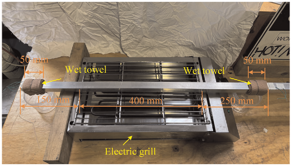
Experimental setup for producing thermal fatigue damage in the square aluminum tube.
The electrical grill is firstly preheated and controlled at a constant temperature of 250°C. Then, the tube is placed above the electrical grill to heat for 40 min, with each surface put at the bottom to heat for 10 min. Subsequently, the tube is kept at a room temperature of 20 °C to cool for 20 min. One thermal cycle consists of 40 min for heating and 20 min for cooling. During the heating process, due to the heat conduction, the temperature of PZTs bonded on the tube could quickly rise. However, because of the heat lose during the heat conduction process, the temperature of PZTs is definitely below 250°C. On the other hand, the material of those shear PZTs is Type Pz27. According to the datasheet on the website provided by the manufacturer, the Curie temperature of Type Pz27 is 350°C, and its recommended working temperature range is below 250 °C. Therefore, theoretically speaking, the PZTs are in the recommended working temperature range. Nevertheless, we are still worried that the high temperature may cause some potential side effects on the PZTs, which may influence the measurement results. Hence, wet towels are used to wrap the area of the tube near the PZTs to block heat conduction. Moreover, during the heating process, some cool water is poured on the wet towels every 5 min. This ensures the temperature of the PZTs remains at a low temperature, which totally avoids the potential effect of high temperature on the performance and functionality of the PZTs.
To confirm two effects of thermal cycles on the square tube, which are the change in microstructures and material properties, Environmental Scanning Electron Microscopy (ESEM) is used to obtain the microstructure images of the aluminum surface for the intact specimen and heated specimen with 10 thermal cycles, respectively. Meanwhile, the Oxford Ultim Max Large Area SSD EDS detector in ESEM is employed to characterize the elemental composition of the intact and heated aluminum surface. Figure 23(a) and (b) show the image of the aluminum surface before and after heating. It is obviously observed that many irregular cavities appear on the aluminum surface of the heated specimen compared to the intact one, which demonstrates the change in microstructure. Figure 23(c) and (d) give the corresponding elemental composition of aluminum surface images, where Wt and
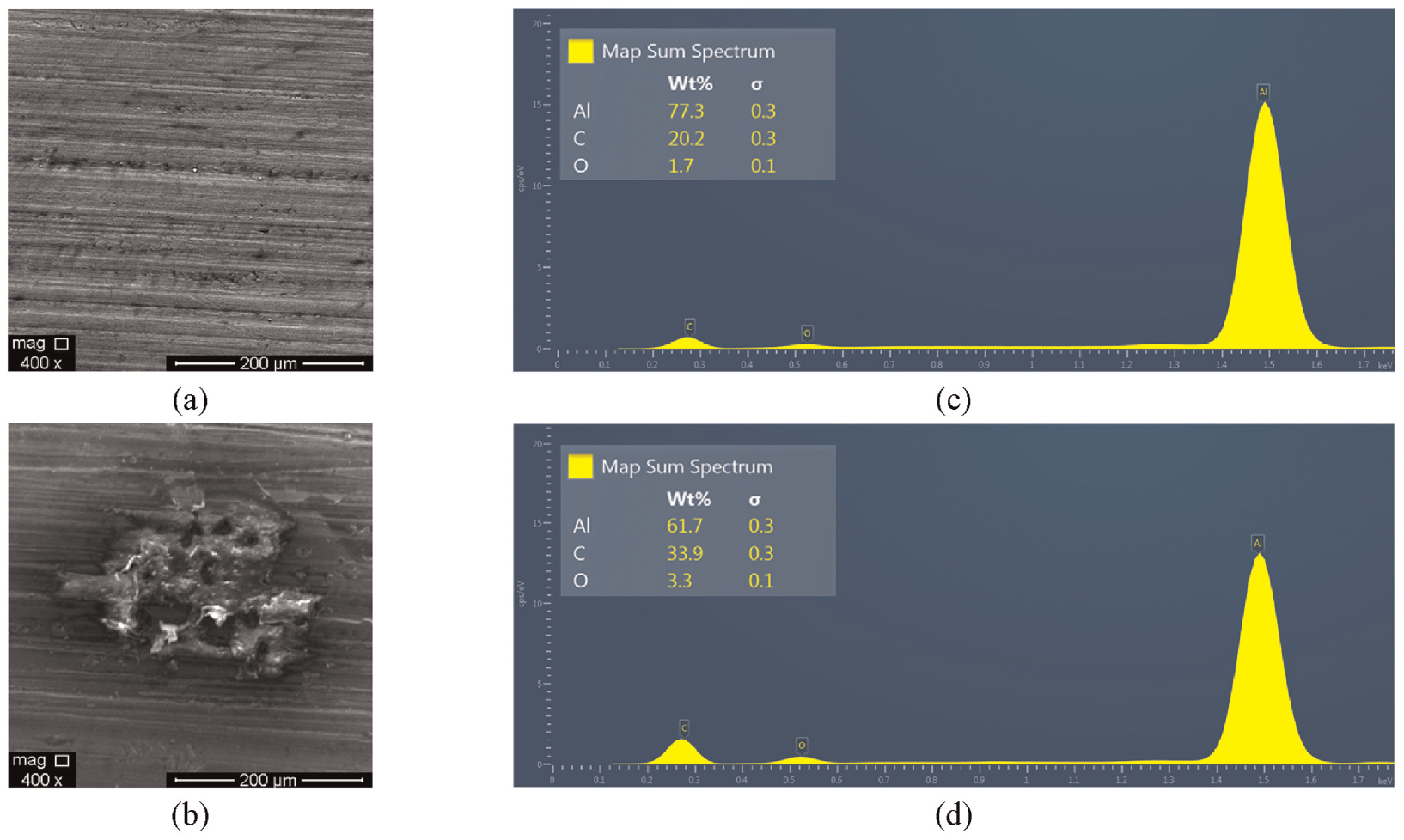
Images of the aluminum surface with 400× magnification and corresponding spectrums of element composition: (a) and (c) intact specimen and (b) and (d) heated specimen.
The specimen is subjected to 10, 20, and 30 thermal cycles with gradually growing thermal cycles to increase the level of thermal fatigue damage. Four times of ultrasonic measurements are performed on the specimen after the specimen is subjected to 10, 20, and 30 thermal cycles, respectively. Figure 24(a) shows the normalized time domain signals of the tube subjected to 0, 10, 20, and 30 thermal cycles. It can be seen that the time domain signals do not have apparent changes compared with the intact ones. Figure 24(b) gives the corresponding frequency spectrum of those signals. It is found that the fundamental waves remain unchanged in amplitude, while the amplitude of second harmonics grows with the increased thermal cycles.
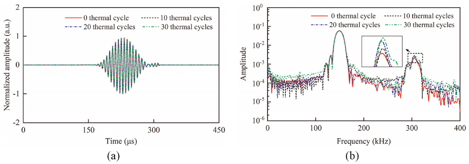
Intercepted experimentally measured signals under different thermal cycles: (a) time domain and (b) frequency domain.
Figure 25 gives the nonlinear acoustic parameter under different thermal cycles. It can be clearly observed that the nonlinear acoustic parameter presents a gradually growing trend with the increase of thermal cycles, which indicates the generated nonlinear guided waves are sensitive to the incipient thermal fatigue damage. Therefore, the proposed second harmonic generation technique is promising for characterizing the early-stage damage in square tubes.
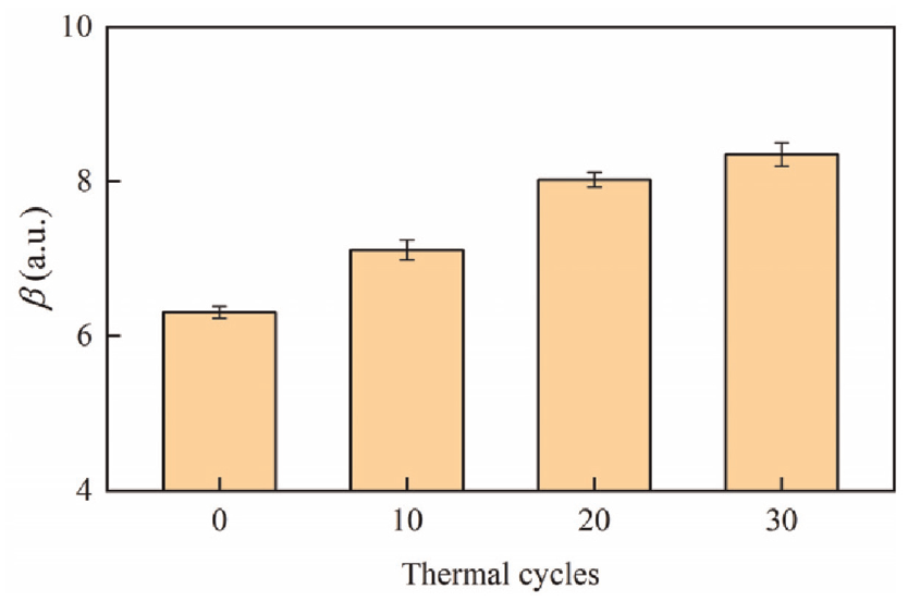
Nonlinear acoustic parameter versus thermal cycles.
Conclusion
In this paper, the second harmonic generation of longitudinal waves in an isotropic square tube with material nonlinearity is studied theoretically, numerically, and experimentally. The main contributions are summarized as follows.
In the rather complicated dispersion characteristics of the square tube, a pair of longitudinal waves, which are subsequently proven to satisfy the internal resonance condition, are found for second harmonic generation. Numerical results indicate the fundamental waves can be well excited. Meanwhile, the induced second harmonics are proven to be cumulative with propagation distance. Then, the ultrasonic measurements are carried out on the square tube with practical PZT configurations proposed for the square tube. The experimental results provide strong support for theoretical and numerical analysis. Finally, the experimental study further employs the generated second harmonics to characterize different severity of thermal fatigue damage in the square tube. The experimental results indicate the nonlinear guided waves are sensitive to thermal fatigue damage. Therefore, the proposed second harmonic generation of longitudinal waves and PZT configurations are very promising for practical application in the detection of incipient damage in square tubes.
Footnotes
Acknowledgements
We would like to express our sincere thanks to Dr. Jingkai Lin (School of Chemical Engineering, The University of Adelaide) for his assistance in Environmental Scanning Electron Microscopy. Besides, the first author would like to acknowledge the scholarship supported by the China Scholarship Council.
Author contributions
Declaration of conflicting interests
The author(s) declared no potential conflicts of interest with respect to the research, authorship, and/or publication of this article.
Funding
The author(s) received no financial support for the research, authorship, and/or publication of this article.