
Abstract
This paper presents a probabilistic model-based optimisation framework for localising and characterising multiple delaminations in laminated composite beams using ultrasonic guided waves (GW). A likelihood-free Bayesian method, approximate Bayesian computation by subset simulation (ABC-SS), is implemented to determine the number of delaminations and identify the unknown damage characteristics and their associated uncertainties. The ABC algorithm provides a practical way to approximate the posterior distributions of uncertain damage parameters and select the most plausible damage model for determining the number of delaminations through direct comparison of the experimentally measured and numerically simulated GW signals without assuming any likelihood functions. To overcome the expensive computational cost of traditional finite element simulations, a higher-order laminated model (HOLM) is employed to model the GW propagation behaviour in the delaminated composite beams with satisfactory accuracy and acceptable computational efficiency. Benefiting from the accurate simulation, the dataset comparison utilises the original time-domain GW signals, thereby preventing the loss of any key information from the signals for damage identification. A comprehensive series of numerical case studies are used to demonstrate the accuracy, robustness and feasibility of HOLM simulation and the proposed multiple-delamination identification framework. The practicability and accuracy of the proposed ABC framework are further validated using two experimental datasets.
Keywords
Introduction
Laminated composite beams
Laminated composite structures generally consist of an assembly of physical layers. These composite materials or structures have wide applications in many engineering fields because of their advantageous characteristics, such as high-strength, lightweight and anti-corrosion. One of the most common categories of defects in laminated materials is delamination.1,2 This would cause a considerable reduction in structural stiffness and may lead to a high structural failure risk. A robust structural health monitoring (SHM) technique for identifying and characterising damages in their early state is essential to ensure structural serviceability and reliability, especially for high-value asset applications, such as aerospace and energy engineering. Depending on the diagnosed location, type and size, engineers can propose a specific maintenance plan and make recommendations for operation. 3 Delamination is considered a type of internal defect that cannot be easily detected using visual inspection. Non-destructive evaluation (NDE) techniques are, therefore, usually utilised in SHM for damage detection and assessment.4–6 Compared with conventional NDE techniques, ultrasonic guided wave (GW) based methods are broadly used for damage detection in composite structures with an increasing trend due to their high sensitivity to local and incipient flaws, the capability of a relatively long propagation distance as well as the ability to inspect inaccessible areas.7–11
Model-based GW approach
To determine the damage location and, in particular, to identify the damage geometry, the model-based GW approach has attracted much attention nowadays due to its baseline-free nature and capability to deal with more complicated damage situations. 12 Specifically, an analytical or numerical model is used to simulate the propagation behaviours of incident waves and their reflection or transmission from the damages, boundaries and interfaces. The damage properties are considered unknown variables and identified by minimising the differences between experimentally measured and numerically simulated GW responses. 13
The ability of the numerical model to predict GW interaction with damages hence plays a vital role in model-based approach. GW propagation could be simulated accurately using the traditional finite element (FE) method with the use of an adequate small element size. Nevertheless, the computational cost is impractical, especially for composite structures, which usually need to be explicitly modelled using numerous elements per layer in order to obtain precise GW damage features.7,9 Different modelling methods have been developed to overcome the limitations of the conventional FE method.14,15 The frequency-domain spectral finite element (SFE) method is computationally efficient compared to the FE method, which utilises spectral analysis techniques to examine structural behaviours at discrete frequencies by solving the partial differential governing equations in the frequency domain.16,17 Time-domain SFE is an alternative that employs Gauss-Lobatto-Legendre (GLL) nodes and high-order approximation polynomials to reduce element number in FE simulation while providing accurate prediction. Runge’s phenomenon can also be prevented by using GLL nodes.18,19 Other advanced techniques, such as semi-analytical FE and hybrid/wave and finite element (WFE), involve the combination of analytical solutions from wave propagation principles and numerical solutions from FE method to obtain the GW scattering features of damage instead of the entire signal, such as reflection and transmission coefficients. Modelling complexity and cost can, therefore, be reduced while the simulation is relatively accurate.20–22 These GW scattering features from damages can then be treated as numerical responses for damage quantification. Additionally, with the rapid development of machine learning and neural networks, surrogate models to predict GW propagation with damage features have also been widely investigated nowadays.23–25 To summarise, while simulation accuracy is of paramount importance, a robust model-based approach must also take into consideration computational effort to remain feasible.
Bayesian GW model-based framework
In addition to the constraint of numerical simulation, the associated uncertainties tend to compromise the efficacy of damage identification. These uncertainties come from various aspects, such as measurement error due to noise from environment and data acquisition systems, modelling error due to model simplification and unspecified material/geometry properties, etc. To accurately define the damage properties and also quantify the involved uncertainties, the Bayesian inference approach was initially utilised in vibration-based SHM and was then extended to GW model-based SHM with a rising tendency.26,27 Bayesian inference considers prior knowledge about the damage and current observations in the model updating procedure. It provides a useful platform to perform online SHM on structures.
Some Bayesian frameworks for GW damage identification can be found in the literature. 28 Ng proposed a model-based Bayesian probabilistic framework with a particle swarm optimisation algorithm for identifying single crack in an isotropic beam structure based on different GW scattering features obtained from different data pre-processing techniques. 29 Yan et al. 30 developed a fast Bayesian scheme with the transitional Markov Chain Monte Carlo (TMCMC) algorithm for damage identification using an analytical probabilistic surrogated model with the WFE to simulate the scattering coefficients. Apart from parameter estimation, the Bayesian approach also provides an essential feature to determine the most plausible model. He and Ng introduced the Bayesian model assessment with TMCMC and subset simulation (SS) to define the unknown number of cracks in beam-like structures.31,32 Different model classes, that is, models with different number of cracks, were assessed by comparing model evidence. Hibert transform of GW signal was used to enhance the sensitivity to identify the corresponding damage geometries. Recently, Cantero-Chinchilla proposed a multi-level Bayesian framework with Asymptotic independence Markov sampling algorithm for damage localisation in plate-like structures. 33 The model class assessment was utilised at the first level to determine the most probable time-frequency (TF) transform technique from raw GW data. Damage localisation with uncertainty quantification was then processed based on the most plausible TF model.
Most studies focused on Bayesian GW model-based approach, despite their effectiveness and rigour, rely on extracting features from GW signals rather than using the entire signal information. Extracting these key features tends to reduce the computational burden as the signal is compressed so that some unnecessary ‘noise’ error can be ‘filtered out’. 29 This works well when the GW damage reflections are simple, for example, in a single-crack situation. Conversely, in complicated damage situations, for example, multiple-damage situations, the signal can be complex as multiple scattered waves are induced by defects, and mode conversion also occurs. The damage reflections are always overlapped and difficult to be separated. Data compression or feature extraction may result in the loss of useful damage information from signals or inevitably introduce additional errors, leading to inaccurate or even incorrect damage identification. 34 Thus, there is still a research gap in developing an accurate and computationally efficient model-based approach using the entire time-domain GW signal to identify damage characteristics.
Approximate Bayesian computation
In Bayesian approach, prior distributions are generally determined based on engineers’ prior knowledge or experience of the damage. Conversely, Bayesian inference also requires defining a likelihood function to measure the level of agreement between predicted and measured responses. 27 The selection of the likelihood function can vary depending on the assumption of uncertainty about the underlying unknown data-generation distribution. In the same damage identification scenario, different likelihood assumptions may result in different posterior distributions of uncertain parameters, that is, different uncertainty quantification results. Additionally, for model simulation involving high-dimensional parameters or complex nonlinearity, the analytical formulation of the likelihood function might be elusive.35–37 As a result, there is no consistent approach that can be applied to all circumstances.
The approximate Bayesian computation (ABC) method, which can bypass likelihood function evaluation, has recently attracted significant attention in the development of a more general and practical probabilistic framework for damage identification. ABC approximates the posterior distributions from the priors by evaluating the similarity directly between the observed and simulated responses.35–37 In this way, ABC still obeys the Bayes theorem principle, while the difficulties of the likelihood function, as mentioned above, are avoided cleverly. ABC can be employed with any forward-simulated model. Some ABC applications can be found in vibration-based SHM for model parameter estimation and dynamic model selection,38,39 while there is limited research in GW-based SHM for damage identification.25,40 Numerous novel ABC algorithms have also been proposed in the last decade to enhance approximation accuracy and reduce computational costs. Some common examples include ABC with Markov Chain Monte Carlo (MCMC), ABC with sequential Monte Carlo (SMC), 38 and approximate Bayesian computation by subset simulation (ABC-SS). 41
To summarise, achieving simulation accuracy is vital to precisely capture GW reflections and scattering. A robust model-based approach must also consider computational effort to remain feasible. It is still worthwhile to develop an advanced FE model that can accurately and efficiently simulate GW propagation within delaminated composites. Bayesian approaches are capable of quantifying unavoidable uncertainties. However, most GW-based Bayesian frameworks were developed depending on different likelihood assumptions, which might limit their applicability. Recently, ABC algorithms have been considered as a more general and practical alternative for model class selection and parameter estimation while still adhering to Bayes’ theorem.
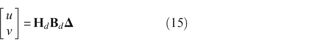
In this paper, a likelihood-free Bayesian framework is developed to identify multiple delaminations in laminated composite beams. An advanced version, ABC-SS, is employed to enhance inference efficiency. In ABC-SS, the SS technique for rare-event simulation is combined with the ABC principle to automatically create a nested decreasing sequence of regions corresponding to an increasingly closer approximation of the observed data, that is, the posterior approximation. ABC-SS algorithm can also evaluate model evidence in a simple by-product manner, which enhances model class selection effectiveness. A higher-order laminated model (HOLM) is also proposed for modelling time-domain GW signals in composite beams. Higher-order deformation kinematics in both thickness and length directions are employed to guarantee simulation accuracy for damage identification. A sub-laminate scheme is used to provide a convenient, efficient and physical way for simulating multiple delaminations while maintaining computation efficiency. SFE and GLL nodes are also used in the model to further reduce computation costs.
The paper is arranged as follows: Firstly, the HOLM formulation and delamination modelling mechanism is provided in section ‘Higher-order laminated model’. ABC-SS and the likelihood-free framework for multiple-delamination characterisation are presented in section ‘Bayesian likelihood-free approach for multiple-delamination characterisation’. Numerical case studies under noise conditions and different numbers of delaminations are used to comprehensively demonstrate the robustness and accuracy of the HOLM and the probabilistic framework in section ‘Numerical case studies’. After that, in section ‘Experimental study’, experimental case studies are employed to further validate the accuracy and practicability of the proposed framework. Conclusions are given in section ‘Conclusion’.
Higher-order laminated model
Formulation of the laminated model GW propagation simulation
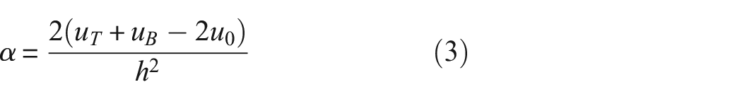
This section presents the proposed HOLM for modelling GW propagation in a multi-layered composite beam. The entire beam is simulated by representing it as a group of HOLM-based sub-laminates, with each sub-laminate containing several physical layers (see Figure 1(a) for an example).
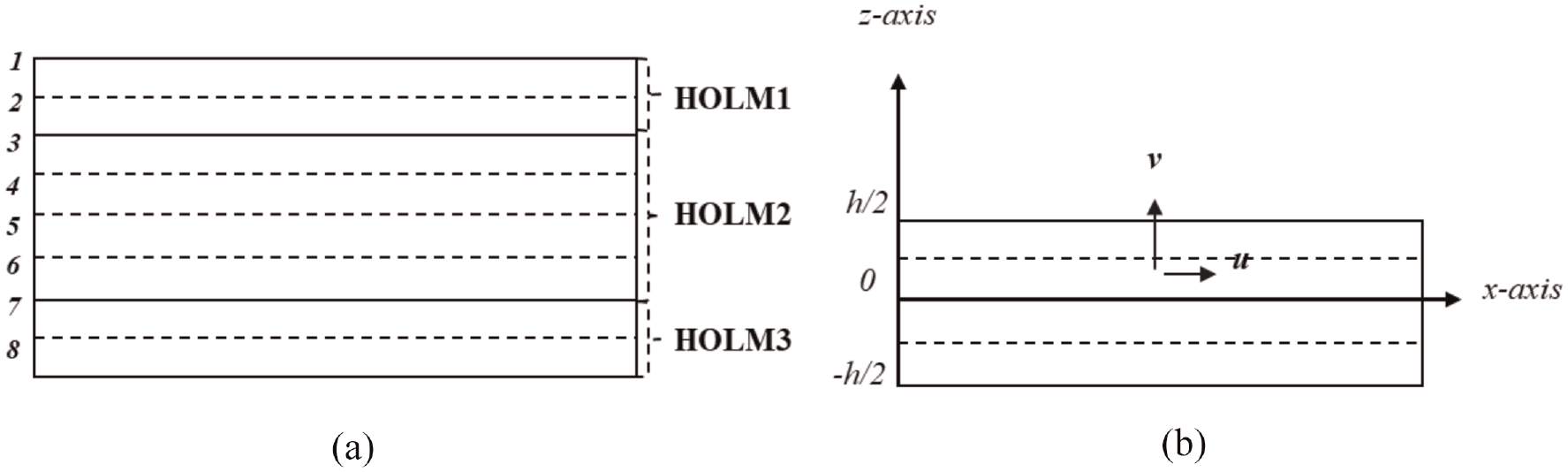
(a) An eight-physical-layer composite beam simulated by three HOLM sub-laminates. (b)
To accurately capture GW propagation behaviour, higher-order through-thickness deformation kinematics is integrated to simulate each HOLM sub-laminate.42,43 As shown in Figure 1(b), the deformation for a sub-laminate is assumed to have a two-dimensional (2D) plane stress condition in the


where
These weighting factors can be expressed by incorporating both
Both


where
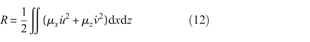
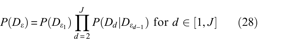
GW propagation simulation is a dynamic problem that can be treated as solving a time-domain ordinary differential equation, also known as the equation of motion. The equation can be derived using the Lagrange equation as below.
where t represents the time.
The main factors of
where
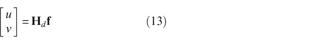
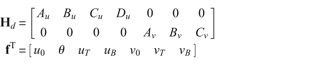
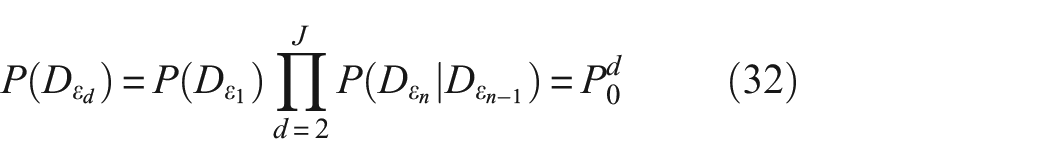
The displacements
where
SFEs with higher-order approximations of the
where
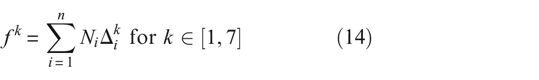
The displacement vector at any nodes of the
where
Following a similar manner, velocities
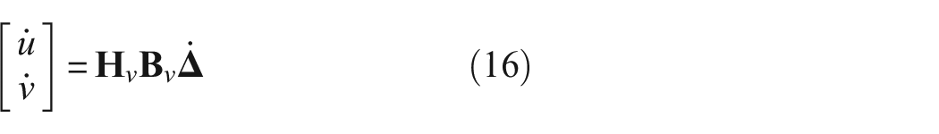
where
The strain vector
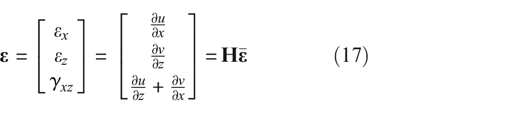
where
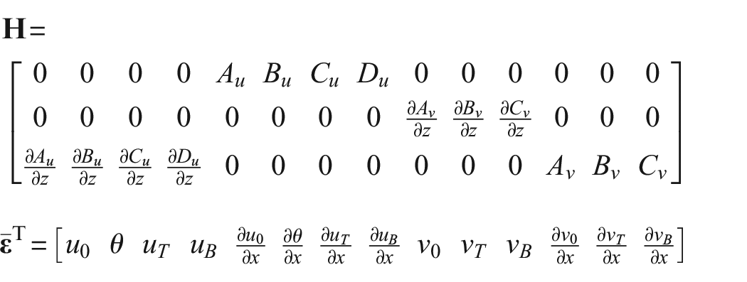
By substituting all displacement vectors

where
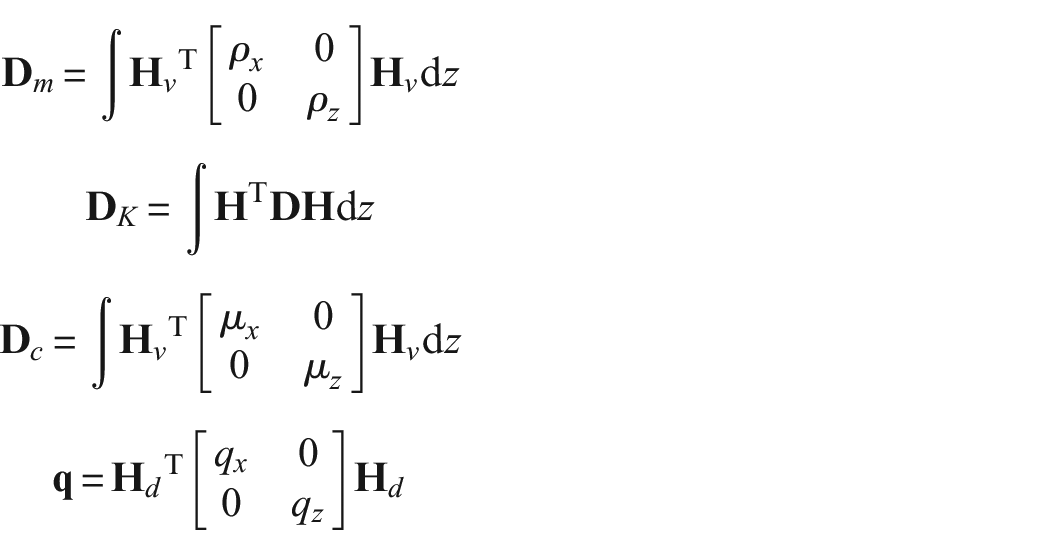
Since the HOLM assumes a plane stress condition in the

By substituting Equations (15)–(19) into Equations (10)–(12), the formulation of the
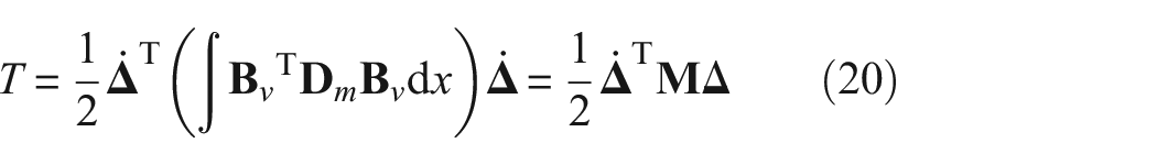
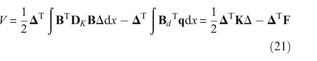
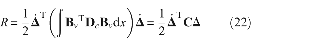
where
The equation of motion for an element of a HOLM sub-laminate can be obtained by deriving the Lagrange equation in Equation (9) after substituting Equations (20)–(22).

where
Delamination modelling scheme
The proposed HOLM considers displacements at both top and bottom external surfaces, providing a simple but physical mechanism to simulate delamination and model multi-layer composite beam (as shown in Figure 2). Specifically, the connection of each sub-laminate HOLM is achieved easily by connecting the same degrees-of-freedom at both upper/lower planes, leading to just one set of nodes in the contact region. Delamination can then be easily inserted into the interface by taking double sets of nodes between two planes. It should be noted that the delamination region can be simulated by using only one or multiple spectral elements, mainly depending on the length of the defect as well as the convergence of the model. Moreover, the proposed composite beam model improves the simulation accuracy in both contact and delamination regions by adopting higher-order variation in the displacement vector and considering multiple HOLM sub-laminates in the thickness direction. The computational efficiency is also enhanced by adopting time-domain SFE and GLL nodes to reduce the number of elements of the entire model, as well as accommodating multiple composite layers (with no delamination) within each sub-laminate.
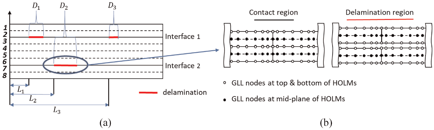
(a) A diagram example of a composite beam with three HOLM sub-laminates and three delamination simulations. (b) The mechanism of contact and delamination simulation at the interface between two adjacent HOLM sub-laminates (incorporating with SFE and GLL nodes).
In this paper, the proposed HOLM is used to simulate GW propagation in composite beam with multiple delaminations. The point load vector in the form of a GW incident pulse is applied to the excitation location of the model. The GW time-domain signals are calculated by solving the equation of motion for the entire beam model using an explicit time integration method, the central difference method. 32
Bayesian likelihood-free approach for multiple delamination characterisation
The procedure of detecting multiple defects using the Bayesian approach typically involves two main stages: mode class selection to determine the number of defects and model updating to identify damage properties, that is, delamination location and severity.31,45 Recall Bayes’ theorem, the posterior distribution for predicting the uncertain delamination parameters
where
At the model class level, given a set of model classes
where
Approximate Bayesian computation
The general idea of ABC is to bypass the likelihood evaluation by directly assessing the similarity between measurements

where the model parameter and model output are simulated from the distribution
For some convenience, for example, high-dimensional datasets or computational burden, summary statistics
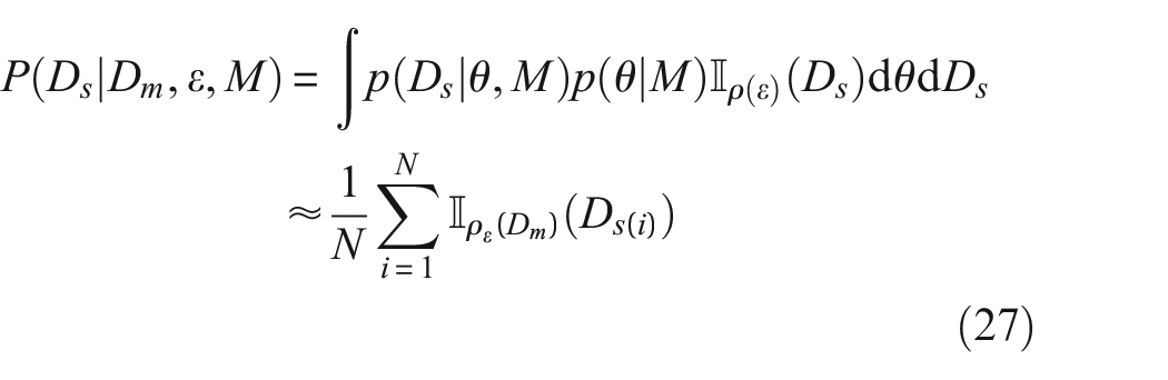
where
It should be noted that the approximation quality of Equations (26) and (27) mainly relies on the choice of distance function
Approximate Bayesian computation by subset simulation
In this paper, ABC-SS will be employed for multiple-delamination identification. It provides a computationally effective way to estimate the evidence of each model class and the posterior of uncertain damage parameters by combining the SS technique with the ABC principle.
41
Specifically, ABC-SS converts the Bayesian inference to a reliability analysis for solving a rare-event problem. The basic procedure involves a sequence of nested decreasing data-approximating regions
where
At the first stage of ABC-SS (
At the simulation stage (
The tolerance level
It is observed that sample size generated in
ABC-SS approximates the posterior probability of the uncertain parameters through an adaptive tolerance procedure until the intermediate tolerance
It is also observed that evidence estimation of the model class at different tolerance levels using ABC-SS is a simple by-product. For a specific

where
where
Implementation of the proposed framework
Some critical factors need to be specified appropriately to guarantee ABC-SS performance. Firstly, ABC model selection is limited due to some constraints, particularly the need for sufficient summary statistics to guarantee sufficiency in all considered model classes. This limitation also directly affects posterior approximations. Different signal-processing techniques to extract GW features from original time-domain signals can be considered summary statistics. Even though data extraction can improve the sensitivity of damage identification, some essential information may be missing, and this would result in inaccurate results. One simple solution to overcome this difficulty is to use the entire measured signals. However, this has a critical requirement for simulation accuracy. 52 In this paper, benefiting from the HOLM, the laminated composite beam simulation can be accurate and close to the actual responses by taking higher-order variation in displacement expressions as well as employing a more physical delamination simulation mechanism. Euclidean distance is chosen as the distance function for assessing the similarity between numerical and measured GW signals, which is commonly used for comparing two same-dimensional data vectors.

The accuracy and efficiency of the ABC-SS are directly affected by MMA, while the Markov chain speed to the convergence state in MMA mainly depends on the spread of proposal PDFs. Assuming Gaussian proposal PDFs, the variance
The selection of conditional probability
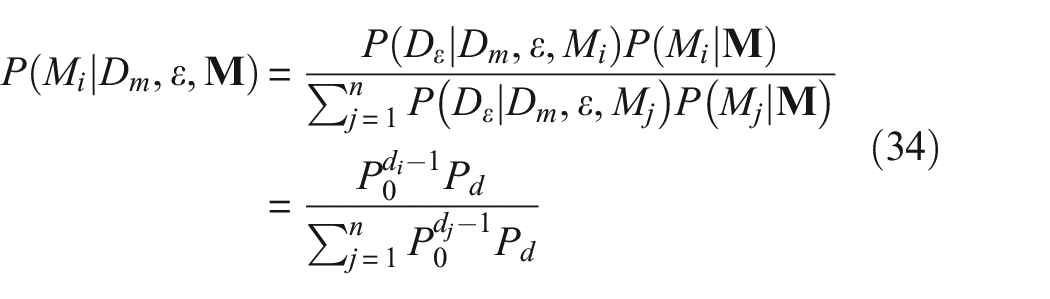
In this paper, the ABC-SS is used to develop a likelihood-free Bayesian framework for multiple-delamination characterisation. A pseudocode implementation of the proposed framework is provided for clear clarification. The details of model class selection and damage parameter identification with evidence evaluation are shown in Figure 3 and Algorithm A, respectively. The HOLM described in section ‘Higher-order laminated model’ is employed to simulate the composite beam with different numbers of delaminations. Once the most plausible delamination number is determined, the corresponding delamination characteristics can be identified. The associated uncertainties can also be quantified by evaluating the posterior distributions.
Damage parameter identification using ABC-SS.
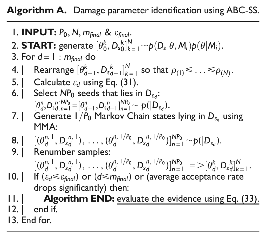
Flowchart of Bayesian model assessment for determining the number of delaminations.
Numerical case studies
Details of the case studies
Different numerical case studies were used to investigate the performance of the likelihood-free probability approach and the HOLM for GW-based multiple-delamination identification. A laminated composite beam with 300 mm of length and 2 mm of total thickness was used. The beam consists of eight equal-thickness composite layers with different fibre orientations: [
Material properties of each identical layer of the laminated composite beam in numerical study.
Delamination details of damage cases in numerical study.
Two case studies were considered for different purposes. Case 1 aims at investigating the convergence of the proposed framework under different noise levels, while Case 2 aims at investigating the performance under multiple-delamination situations. The incident was selected as the fundamental asymmetrical mode (A0) of GW because of its sensitivity to defects.
31
The excitation was applied at the top surface of the left end of the beam in the transverse (
The HOLM was used for simulating numerical GW signals. Based on an initial convergence study, 15 mm-long SFE was used for beam modelling.
42
Eight GLL nodes per element and time step of
A commercial Finite element modelling (FEM) software, ABAQUS (Version 6.14, DASSAULT SYSTEMS, Paris, French), was also employed to build laminated models for generating synthetic experimental GW signals. Assuming that the beam is 6 mm wide and 300 mm-long. 3D solid brick elements (C3D8R) were used to simulate composite beams. The excitation and measurement locations were same as the HOLM setting, and the load was acting across the entire width. The delamination region and intact region between layers were simulated using ‘untie’ and ‘tie’ connection constraints at the corresponding locations. The mesh size was 0.2 mm to ensure simulation convergency in all directions, and the time step was automatically defined by the dynamic explicit solver. Measurement error for GW experiment under the laboratory condition was also considered by adding different signal-to-noise levels to the synthetic signal. All captured time-domain signals from both HOLM and ABAQUS were normalised based on the maximum amplitude of signal for comparison.
In terms of prior distributions for each uncertain parameter, assuming early stage of damage, the prior distribution of location
Case 1: single delamination with different measurement noise levels
This section investigates the ABC framework performance under various measurement conditions. The noise level from 2.5% to 7.5% is assumed to represent normal to adverse laboratory conditions. Figure 4 shows the time-domain GW signals generated from both the commercial FEM and the HOLM. In Case 1, only one delamination was considered. As can be observed, GW damage reflections can occur twice in the delamination region when the wave enters and exits the damaged area. The amplitudes of damage reflection tend to depend on defect size and also on the layer-wise location. Even though the length in Case 1 is only 6 mm, the reflection energy reflects that A0 is sensitive to detect delamination in composite. According to Figure 4, there is little shifting error between the two signals due to modelling error (2D modelling from HOLM and 3D modelling from ABAQUS), but overall, there is good agreement between the signals. This simulation illustrates the accuracy of the proposed HOLM.
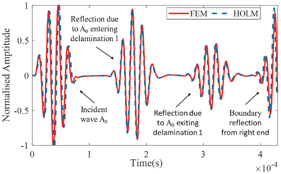
Time-domain signals from FEM (in red with solid line) and HOLM (in blue with dot line) at measured location in Case 1.
The tolerance level is determined adaptively in the ABC-SS algorithm. For clear illustration, the distance function evaluation at each stage for M1 in Case 1a is presented in Figure 5(a). Samples were rearranged in ascending order based on the value of the distance function. The dynamic tolerance in each stage
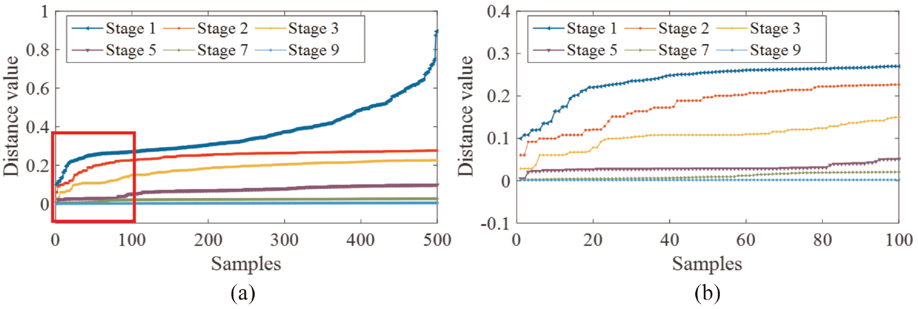
(a) Rearranged samples in ascending order based on distance function values at each stage at M1 in Case 1a. (b) Zoom-in details (red rectangle) of the 100 selected seeds at each stage in ABC-SS.
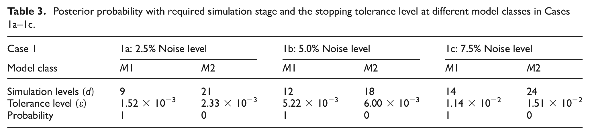
When either of the stopping criteria was reached, the algorithm was terminated, and the required simulation stage and stopping tolerance could be determined. The posterior probability was then calculated from Equation (34). As shown in Table 3, since the first model class has the highest probability, only two model classes, that is, single delamination and two delaminations, were involved in the model class assessment. It was observed that more stages were required to reach the optimum with the increasing noise effect. The stopping tolerance level was also increased due to more uncertainty involved in parameter estimation. Despite that, as highlighted in Table 3, the delamination number was accurately predicted.
Posterior probability with required simulation stage and the stopping tolerance level at different model classes in Cases 1a–1c.
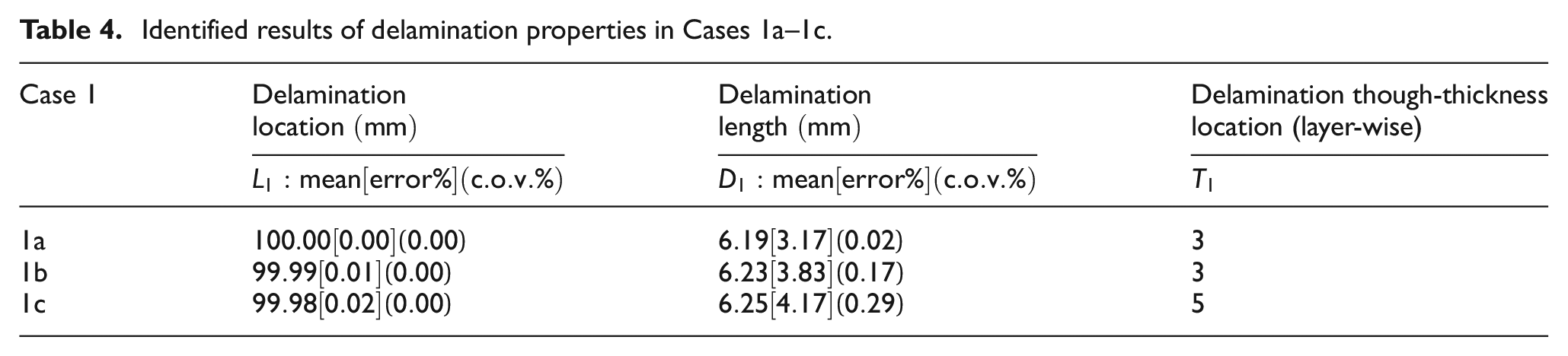
As shown in Table 4, delamination properties in Cases 1a–1c were accurately identified. Since the GW reflection was affected by a higher noise level, a larger uncertainty level was quantified in the parameters, especially in the delamination length. The error percentage between the prediction and the exact value was increased from 3.17% to 4.17%, as well as the coefficient of variation (COV) value was increased from 0.02 to 0.29.
Identified results of delamination properties in Cases 1a–1c.
Similar behaviours were observed in the scatterplots of the 500 samples (see Figure 6). These samples transitioned from the prior distribution and gradually to the posterior distribution. As the noise level increased from 2.5% to 7.5%, there was a relatively larger region for the global optimum, particularly for the length parameter. However, the overall quantified uncertainty in each case remained acceptable and within expectations. This was attributed to the large A0 GW reflection energy from delamination, which reduced the impact of noise effects.
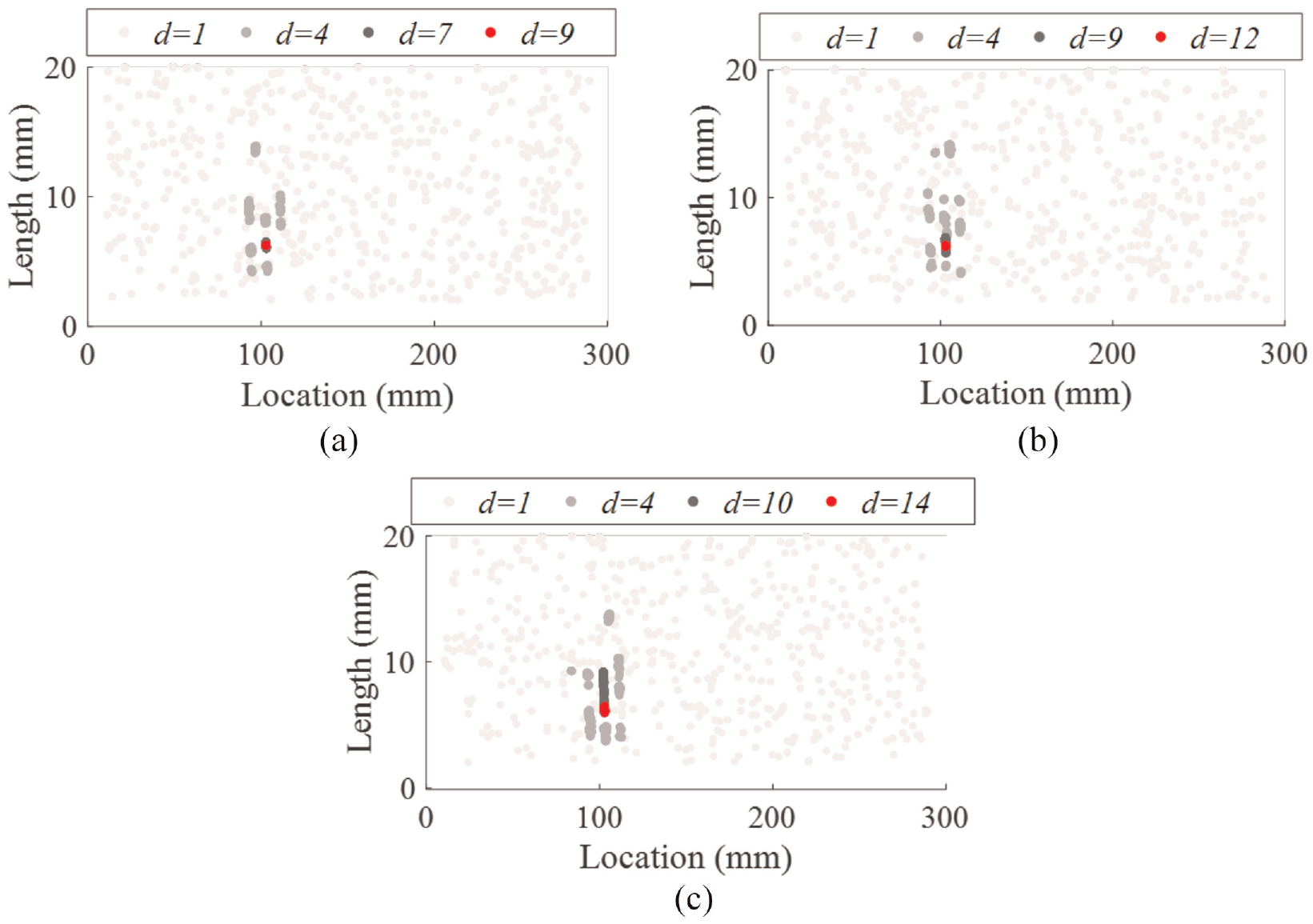
2D scatterplot of the 500 samples (delamination lengthwise location
Case 2: multiple delaminations with 2.5% of measurement noise level
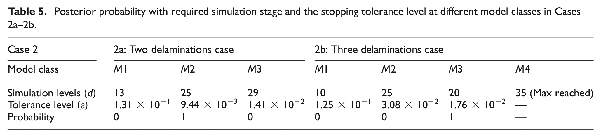
This section further examines the proposed framework performance under multiple-delamination situations. The number of simulation stages and the final stopping tolerance levels in Cases 2a–2b are summarised in Table 5. Given the increased complexity of the GW signal due to additional damage reflections from multiple delaminations, it was expected that more simulation stages would be necessary than Case 1 to calibrate the unknowns and minimise discrepancies between simulations. More model classes were also involved in both cases until the highest posterior probability was determined. For clear illustration, Figure 7 displays the ABC model evidence calculated from Equation (33) in Case 2a against the dynamic tolerance level, along with the comparison of posterior probabilities calculated from Equation (34).
Posterior probability with required simulation stage and the stopping tolerance level at different model classes in Cases 2a–2b.
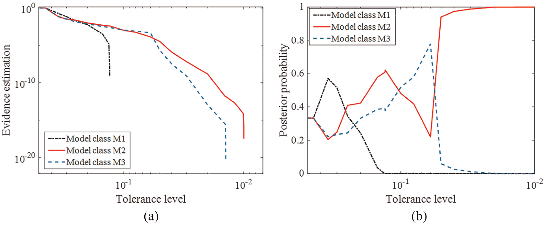
(a) ABC evidence estimation and (b) the posterior probability of all three considered model classes against the dynamic tolerance level in Case 2a from the initial to the final simulation stage.
Referring to the information-theoretic point of view for log evidence, the posterior probability computation considers a trade-off between two terms. The first term measures the posterior average data fit of the model class. The second term is defined as the relative entropy between the prior and posterior distributions, and it measures the extracted information about the model class complexity.53,54 In short, an optimal model class tends to have an acceptable average data-fitting accuracy while extracting less information about its model parameters. It was found that posterior probability estimation using ABC-SS follows a similar concept to define the preferred model. Specifically, the tolerance level determined from the distance function provides a similar way to measure the goodness of fit. At the same time, the number of simulation stages reflects the overall penalty on the complexity of the model class, that is, more simulation stages are required in a more complex damage scenario.
Following the aforementioned rule, it was observed from Table 5 and Figure 7(a) that M1 in Case 2a has the smallest complexity penalty, as it requires the fewest simulation numbers to reach the final stage. The phenomenon makes sense as M1 only considers a single-delamination scenario. Nevertheless, M1 was unable to achieve good data-fitting accuracy, such that the algorithm is stopped at a relatively large tolerance level compared to other considered model classes. The posterior probability of M1 dropped and eventually became zero as the dynamic tolerance level decreased (see Figure 7(b)). In contrast, M2 was accurately selected as the optimal class due to achieving the best data-fitting accuracy (i.e., the smallest tolerance) while only extracting less information about the model class complexity than M3. In a similar manner, the number of delaminations in Case 2b was also accurately detected as M3, that is, three delaminations. It should be noted that M4 was excluded from model class assessment, as the algorithm was stopped at the maximum stage.
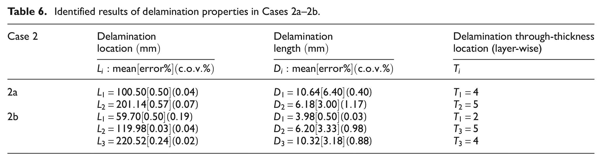
The uncertain parameters in both cases are summarised in Table 6. In terms of quantified uncertainty, the error percentage and COV values increased compared to Case 1. This is because the GW reflection signal was more complicated, and more reflections were generated from defects. This led to more noise effects or uncertainties involved in damage identification. Nevertheless, all delamination parameters were accurately identified with acceptable errors. The time-domain signals from FEM and HOLM (using the mean value of identified parameters in Table 6) are also presented in Figure 8 for comparison. Some reflection pulses, as observed were overlapped in an irregular wave shape, containing combined damage information from different delaminations. There is overall good agreement between the two simulations, indicating accurate multiple-delamination identification.
Identified results of delamination properties in Cases 2a–2b.
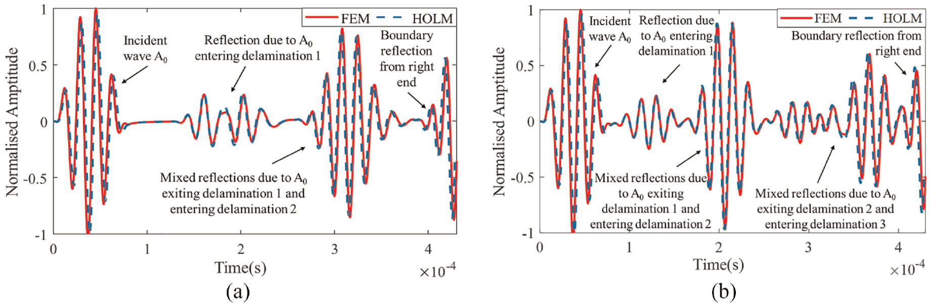
Time-domain signals from FEM (in red with solid line) and HOLM (in blue with dot line) at measured location in (a) Case 2a and (b) Case 2b.
Figure 9 presents the histograms for delamination lengthwise locations and lengths at the final stage in Case 2b for illustration. The posteriors were distributed close to the exact value in each parameter. It was also observed that the posteriors approximated by ABC algorithm showed different types of statistical distribution, reflecting that uncertainty error has different impact on different parameters. The associated uncertainties can be quantified by evaluating distribution shapes. The histogram range was consistent with the corresponding error percentage and COV value shown in the summary Table 6.
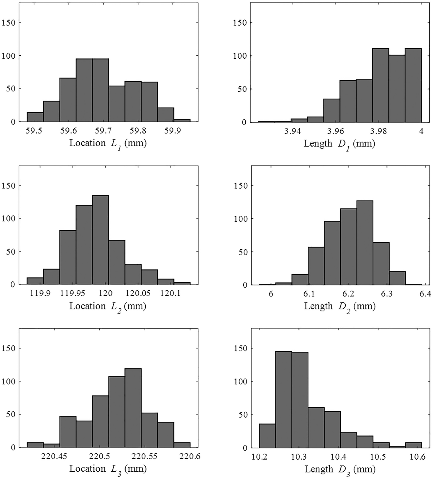
Histograms for all delamination lengthwise locations
Experimental study
Experiment setup
Two fibre-reinforced polymer beams with 6 mm width were utilised in the experimental study to validate and investigate the practicability of the proposed likelihood-free framework. The Beams were made by eight HexPly M21/IM7 (Hexcel) carbon and epoxy physical layers with an assembling orientation of
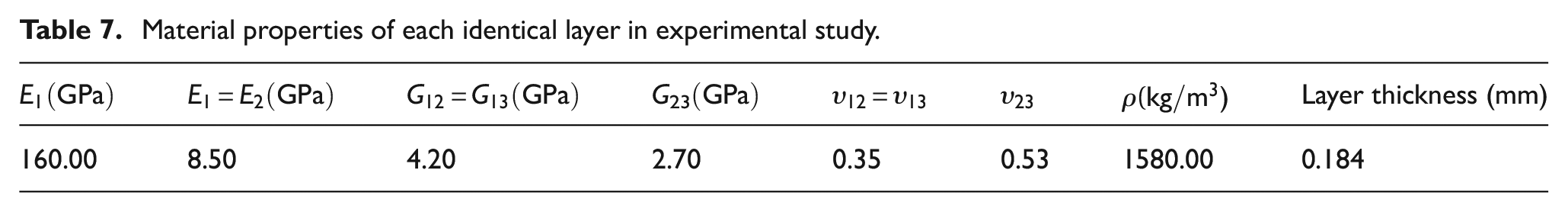
Material properties of each identical layer in experimental study.
A similar experimental setup as He and Ng
32
was conducted in this study. Specifically, both ends of the beam were fixed using rigid clamps. The length of the beam between the two clamps is 300 mm. A plate piezoceramic transducer (PZT) with dimension
The excitation was generated using a signal generator NI PXIE-5412 and then amplified by a high-voltage amplifier before applying to the PZT. The transverse displacement
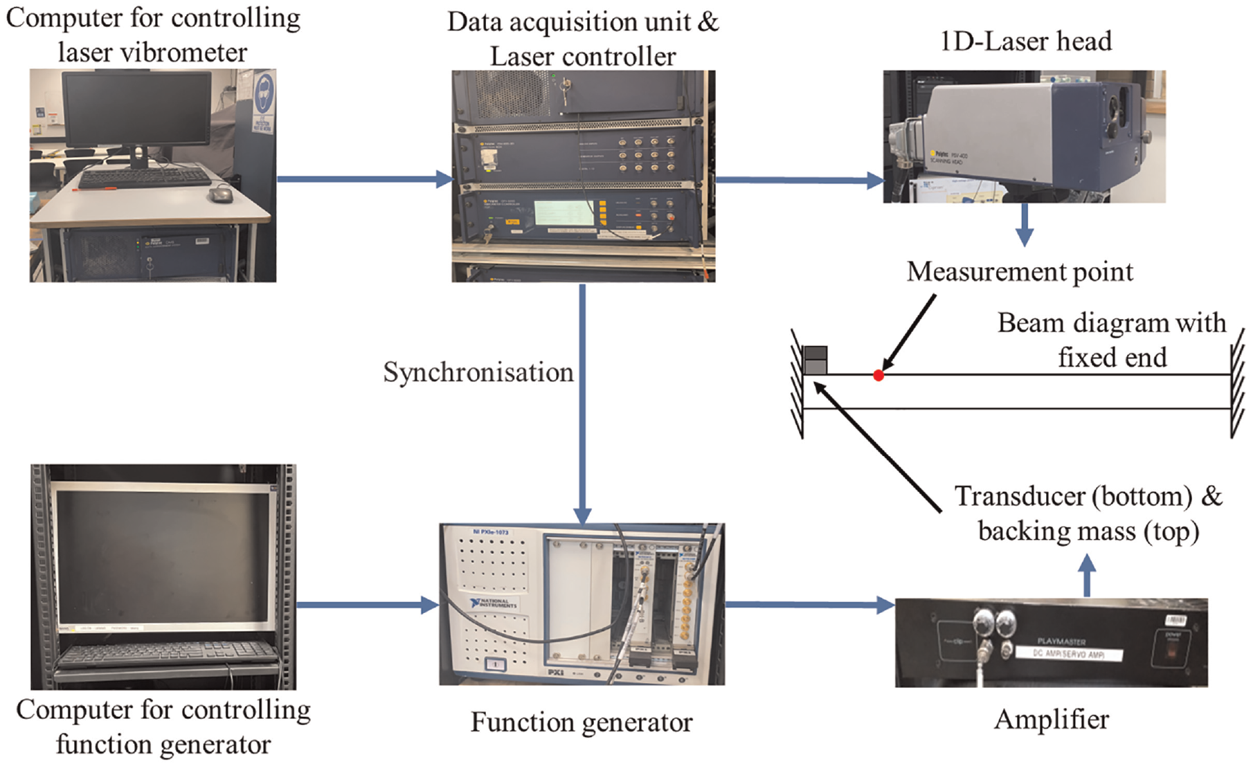
Detailed experimental setup of GW excitation using transducer and measurement using 1D laser.
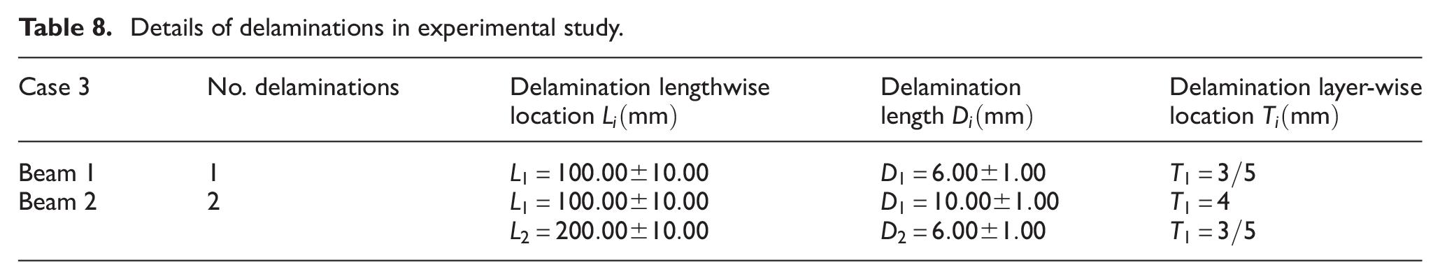
Details of delaminations in experimental study.
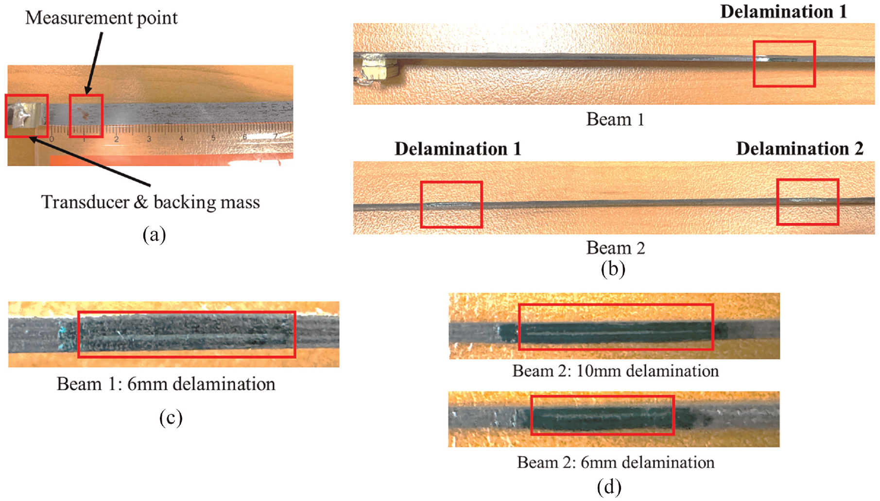
Details of (a) PZT installation and measurement location, (b) delamination locations in beam 1 and beam 2, (c) zoom-in detail of 6 mm delamination in beam 1 and (d) zoom-in details of 10 mm and 6 mm delamination in beam 2.
Results and discussions
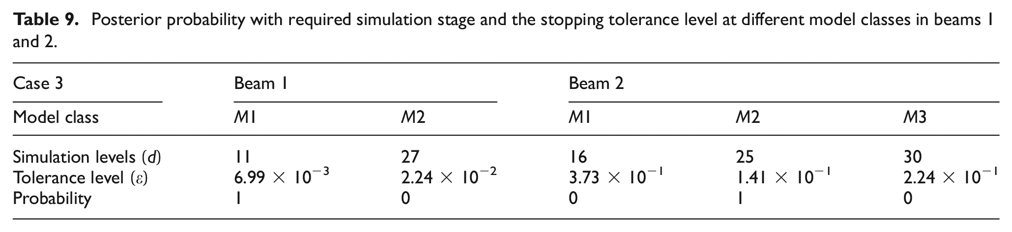
The same HOLM and ABC-SS algorithm settings in numerical study were employed in both experimental studies. Table 9 summarises the number of simulation levels and the corresponding final tolerance level for both experimental cases. Different model classes were automatically considered based on the proposed flowchart in Figure 3 until the highest probability was obtained. M1 in Beam 1 and M2 in Beam 2 were selected as the most plausible model due to the best goodness of fit (i.e., the smallest stopping tolerance) and less model complexity penalty (i.e., less simulation stages). The number of defects in both cases was correctly identified as one delamination in Beam 1 and two delaminations in Beam 2.
Posterior probability with required simulation stage and the stopping tolerance level at different model classes in beams 1 and 2.
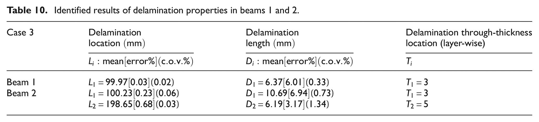
A summary of the identified delamination properties can be found in Table 10. The results are presented as sample mean at the final stage. The corresponding percentages of error and the sample COV are also included. Although the layer-wise location in Beam 2 differed by one layer from the actual location, most of the delamination properties were identified accurately. A comparison of the time-domain GW signal for Beam 1 between the measurement and the simulation (using the mean value of identified parameters in Table 10) is presented in Figure 12 for illustration. In addition to the excitation pulse, two GW damage reflections due to the wave entering and exiting the delamination zone were clearly captured in the measurement. As observed, both GW signals from simulation and measurement were highly matched, while the uncertainty level was also well-controlled during measurement. The quantified uncertainties, as shown in Table 10, were acceptable and within expectations. The accuracy of multiple-delamination identification in both experimental studies further validated and demonstrated the practicability of the proposed likelihood-free framework.
Identified results of delamination properties in beams 1 and 2.
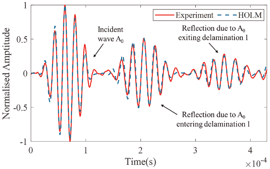
Time-domain signals from experiment (in red with solid line) and HOLM (in blue with dot line) at measured location in Beam 1.
Figure 13 shows the 2D scatterplots for the delamination lengthwise locations and lengths in Beam 2 from the initial stage to the final stage. With the number of iterations increasing, 500 samples were moved from a wide initial range to a small search area and eventually arrived at the global optimum. The size of the optimum region mainly depends on the uncertainty effects of the unknowns from both measurement and simulation. It was observed that the final scattering areas in both delamination lengths were relatively larger than the ones in both locations, demonstrating that more uncertainties were involved in the length parameter estimation procedure. But overall, the uncertainties were well-controlled, which allowed the optimisation to identify delamination parameters precisely within acceptable error margins and refine global optimums.
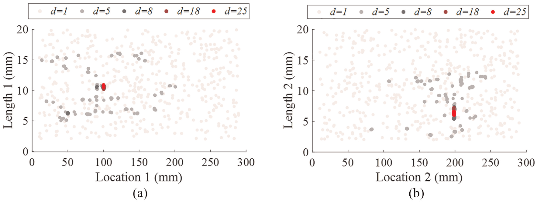
2D scatterplot of the 500 samples (delamination lengthwise locations vs lengths) (a)
The posterior distributions at the final stage in Beams 1–2 are also shown in Figure 14 using histogram plots for better observation. The posterior samples were well-established around the actual value within acceptable error margins. By evaluating the statistical properties of each posterior distribution, the associated uncertainties were quantified, and also the error information provided reliability of the identified results. Figures 13 and 14 further demonstrated the accuracy and practicability of the proposed framework for multiple delaminations in composite in laboratory practical application.
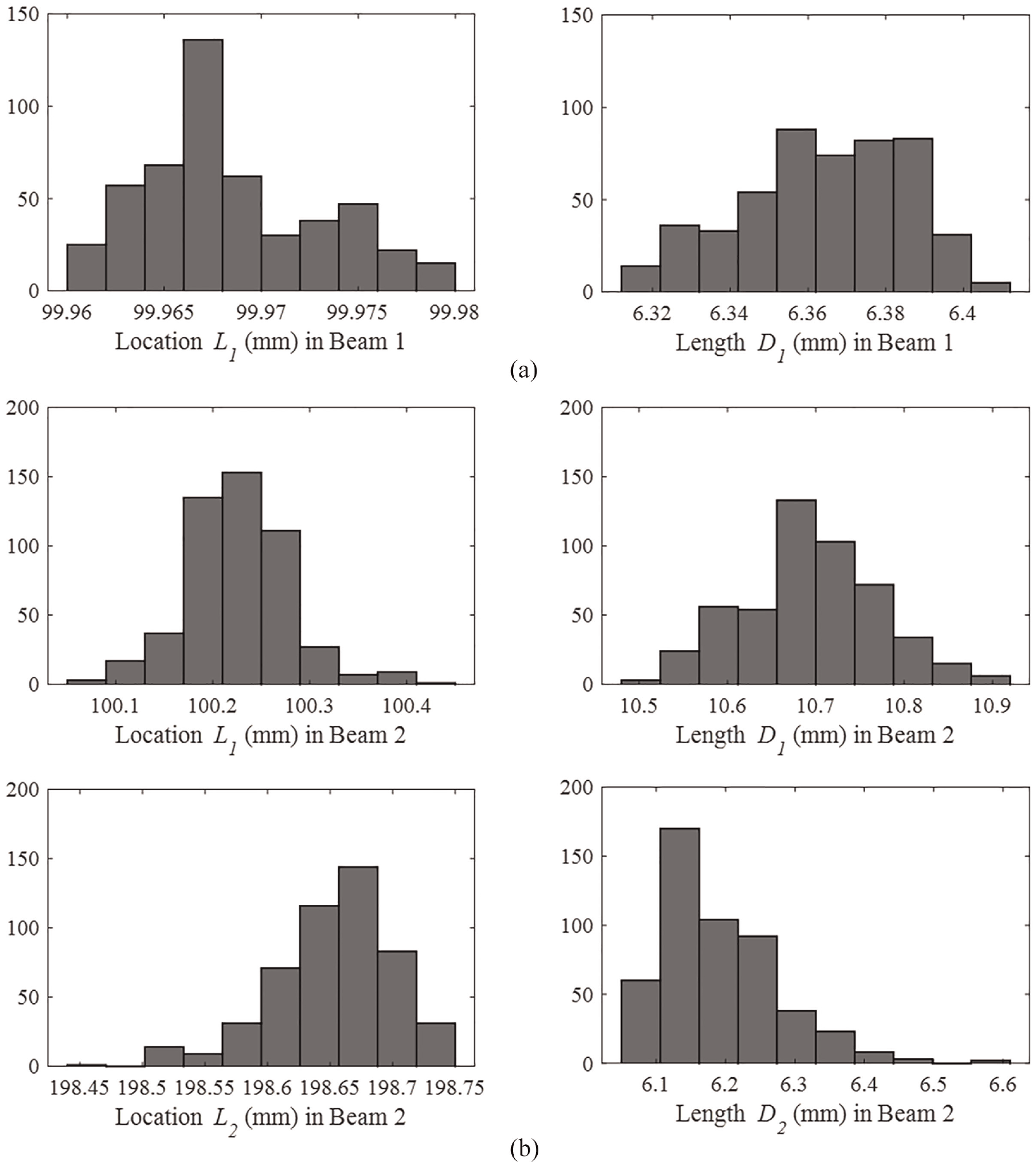
Histograms for all delamination lengthwise locations
Conclusion
This paper proposed a GW model-based approach for characterising multiple delaminations in composite beams. The proposed framework incorporates a likelihood-free method, the ABC-SS algorithm, which provides a straightforward and practical alternative to Bayesian model selection and parameter inference without assuming any likelihood functions. Model evidence estimation of a model class is a simple by-product of ABC-SS algorithm. This provides a clear understanding of selecting the most plausible model using ABC approach. Instead of using any GW signal-processing techniques, damage identification in this study relies on the entire GW time-domain signal. A HOLM with a sub-laminate scheme is used to enhance the simulation efficiency and accuracy of GW propagation in composite beams. A cubic variation of in-plane displacement and a quadratic variation of transverse displacement expression over the beam thickness were employed. This allows delamination to be simulated by simply connecting or disconnecting the corresponding nodes at the top and bottom surfaces of the adjacent sub-laminates. The numerical studies have comprehensively demonstrated the procedures to identify multiple delaminations using ABC model selection and parameter estimation. The HOLM has also proven that precisely simulate GW propagation behaviours from delaminations compared to traditional FE methods, minimising the impact of modelling uncertainties on identification results. Two experimental studies have further verified the accuracy and practicability of proposed ABC framework in laboratory applications.
The current approach has great potential for identifying delaminations in any composite structures. However, different stacking materials may lead to different GW damage responses and more complex reflection signals. More associated uncertainties in real situations can also be involved compared to controlled laboratory conditions. The presented HOLM is capable of simulating any composite beam by applying relevant material properties and orientations. Further research is necessary to examine the proposed ABC framework in real applications. The current study only considers Euclidean distance as a similarity measure, while other distance functions could be explored to account for various aspects of captured wave signals. Further research is needed to examine the impact of ABC damage identification on the selection of different distance functions. The proposed framework can also be used with any numerical model to identify specific defect types of interest. In addition to defining the number of defects, ABC model selection can be used to classify defect types if sufficient damage information is available from measurement. Further research is worthwhile to enhance the applicability and practicability of the ABC framework in GW model-based damage identification.
Footnotes
Declaration of conflicting interests
The author(s) declared no potential conflicts of interest with respect to the research, authorship and/or publication of this article.
Funding
The author(s) disclosed receipt of the following financial support for the research, authorship and/or publication of this article: This work was funded by the Australia Research Council (ARC) under grant numbers DP210103307 and LP210100415. The support is greatly appreciated.