
Abstract
This paper proposes a data-driven approach to detect damage using monitoring data from the Infante Dom Henrique bridge in Porto. The main contribution of this work lies in exploiting the combination of raw measurements from local (inclinations and stresses) and global (eigenfrequencies) variables in a full-scale structural health monitoring application. We exhaustively analyze and compare the advantages and drawbacks of employing each variable type and explore the potential of combining them. An autoencoder-based deep neural network is employed to properly reconstruct measurements under healthy conditions of the structure, which are influenced by environmental and operational variability. The damage-sensitive feature for outlier detection is the reconstruction error that measures the discrepancy between current and estimated measurements. Three autoencoder architectures are designed according to the input: local variables, global variables, and their combination. To test the performance of the methodology in detecting the presence of damage, we employ a finite element model to calculate the relative change in the structural response induced by damage at four locations. These relative variations between the healthy and damaged responses are employed to affect the experimental testing data, thus producing realistic time-domain damaged measurements. We analyze the receiver operating characteristic curves and investigate the latent feature representation of the data provided by the autoencoder in the presence of damage. Results reveal the existence of synergies between the different variable types, producing almost perfect classifiers throughout the performed tests when combining the two available data sources. When damage occurs far from the instrumented sections, the area under the curve in the combined approach increases
Introduction
Structural health monitoring (SHM) is gaining importance for bridge managers and researchers.1,2 In the last decades, many bridge structures have been instrumented to monitor their response during operation.3–10 Instrumentation systems are often deployed in structures to track specific processes (e.g., construction steps and concrete hardening phenomena). Sometimes, these devices are removed from the structure after completing the target task and turn unprofitable. In other cases, the instrumentation systems remain installed but are inactive or disregarded. Under such scenarios, different sensor types coexist in the same structure, offering redundant and complementary information on the structural condition. From a value of information perspective, a continuous SHM strategy based on measurements obtained from these devices efficiently exploits their assessment potential throughout adequate processing.
One of the most critical tasks in SHM is damage detection.1,11 Civil engineering structures are subject to several deterioration processes, including material degradation, aging, and extreme loading conditions. 12 Damage detection is an inverse problem that indicates the structural health condition from measurements.13,14 Two main approaches exist in damage detection: model-based and data-driven. 12 Model-based approaches employ computational models to account for the physics governing structural behavior. 13 Model-based SHM is extensively employed given its ability to reach high damage identification levels according to Rytter scale, 15 allowing to locate and quantify the damage. The Rytter scale classifies SHM algorithms based on the reached level of damage characterization, where four levels exist: (I) detection, (II) location, (III) quantification, and (IV) prognosis.15,16 These techniques require strong physical knowledge and modeling skills.14,17 Besides, the iterative procedure required to solve the inverse problem of damage identification involves running thousands of simulations with the corresponding computational expense. This situation prevents model-based approaches from yielding a fast assessment close to real-time once new data are measured.14,18
By contrast, data-driven techniques assess the health condition of structures based uniquely on monitoring data.11,12 These approaches skip the need for complex models based on engineering knowledge and the associated computational cost to solve the identification problem. However, monitoring data regarding possible damage conditions is rarely measurable in real practice, and only healthy data are available. When only healthy measurements are employed, the SHM approach consists of characterizing the baseline condition (healthy) and detecting departures from this reference, which corresponds to level I in the Rytter scale. 15 The core idea of data-driven methods is thus to characterize the reference (undamaged) behavior of the structure and detect an outlier when a novelty (i.e., damage) occurs.11,19
One of the most challenging issues in data-driven methods is tackling the effect of changing environmental and operational conditions (EOCs).14,20,21 These phenomena (e.g., temperature, humidity, traffic) may mask the presence of damage and hinder the ability of the algorithms.22,23 Numerous statistical methods have been developed to address this problem, such as autoregressive models 17 or Principal component analysis (PCA).23–26 PCA is a statistical data compression tool widely employed in outlier detection for SHM.7,27–29 This method allows isolating environmental and operational variability by projecting the data onto the most relevant principal components (eigenvectors) of the covariance matrix. 30 However, PCA is mainly restricted to linearly correlated data spaces, which limits its applicability.
The emergence of artificial intelligence introduces new techniques to handle large amounts of data and account for complex nonlinear relationships.31,32 Machine learning has progressively extended to many application areas, including the identification of structural damage.33–36 Neural networks (NNs), and particularly deep neural networks (DNNs) have demonstrated to be powerful techniques in SHM applications.32,37–46 convolutional neural networks (CNNs) have demonstrated powerful performance as image processing techniques to detect external damage. 32 For example, in Cha et al., 47 authors employ a CNN that automatically learns image features to identify cracks in concrete. It incorporates a sliding window technique to accommodate different image sizes. They design the CNN to classify images and detect the presence of cracks robust to image noise sources. Cha et al. 48 propose an enhanced approach to identify different damage types (cracks, corrosion, and delamination) by applying a faster region-based CNN. In contrast to traditional statistical methods, NNs require a training phase to learn relationships from large amounts of data. 31
In the line of damage detection accounting for varying EOCs, many DNN-based works have been proposed. 32 One of the most powerful methods in this task is the autoencoder. 49 Autoencoders are a specific neural network type based on the same idea of data compression as PCA but include nonlinearities. 50 An autoencoder reconstructs the input data by following two steps: encoding and decoding. 51 The encoding step compresses the data onto a lower-dimensional latent representation (dimensionality reduction), and the decoding step reconstructs the original measurements from the lower-dimensional features. 52 During training, the autoencoder learns to reconstruct data from the healthy condition of the structure. The healthy condition consists of long-term monitoring data that includes environmental and operational variability. 40 By learning the existing relationships in the long-term monitoring data that is affected by EOCs, we ensure that this variability is considered to be “normal,” thus establishing a reliable description of the reference behavior.8,38 The reconstruction error measures the discrepancy between a measurement and its reconstruction. When new measurements are obtained that belong to a similar (undamaged) condition, we expect that the autoencoder will adequately reconstruct them with a small error value. We assume that the damage-induced variability affects the data differently than environmental and operational phenomena. 53 Thus, we expect that the autoencoder yields a high reconstruction error with the appearance of damage that sufficiently affects the measurements.8,38 Several works exist in the literature employing reconstruction error in SHM applications.8,36,37,49,54 For example, Bao et al. 55 propose a two-step damage detection approach that transforms raw data signals into grey-scale images and trains a DNN based on stacked autoencoders. The recent work 56 employs autoencoders to produce two reconstruction error metrics indicative of damage. Article 57 proposes an adversarial autoencoder trained with vehicle acceleration responses and uses the reconstruction error as the damage indicator. In Lee et al., 58 authors employ a convolutional autoencoder for damage detection on a PSC-I bridge under vehicle-induced excitation using acceleration signals. In Amarbayasgalan et al., 54 authors propose a deep autoencoder for an efficient dimensionality reduction and then apply a density-based clustering for outlier detection. In this work, we employ an autoencoder DNN to reconstruct monitoring data subject to EOCs and employ the reconstruction error as the damage-sensitive indicator.
Another critical aspect of data-driven approaches is to identify the variables to measure. Vibration-based are the most extensively employed data.9,17,46,53,59 In this context, raw vibration measurements (e.g., acceleration signals) are often processed through operational modal analysis (OMA) 60 techniques to produce the modal properties of the structure, mainly eigenfrequencies and eigenmodes. 23 These are strongly sensitive to the presence of damage23,61 Avci et al. 17 reviewed the extensive literature on different data-driven approaches to detect structural damage using vibration monitoring data. For example, in Bakhary et al., 62 authors employ eigenfrequencies and eigenmodes as the input features to estimate the location and severity of damage by applying a two-stage NN incorporating system substructuring. They validate the method in small-scale concrete slab and steel-frame structures. Particularly on bridge applications, Xu et al. 63 propose a two-step approach employing a modal energy-based damage indicator to locate damage and estimate its location with a NN. In Jayasundara et al., 64 authors employ modified modal strain energy and modal flexibility versions as the damage-sensitive features to feed a four-layer NN that estimates damage location and severity. Azim and Gül 65 employ two parallel approaches to detect and locate damage in the beams and the deck of a bridge. They employ the modal strain energy as the feature to find a damage indicator for the steel beams and the relative flexibility change for the reinforced concrete deck. Nick et al. 66 also employ a damage-sensitive index based on modal strain energy calculated from the first three bending eigenmodes to detect and estimate the location of damage in steel girder bridges. They apply a NN to quantify the damage that is trained with synthetic data from a computational model. In Wickramasinghe et al., 67 authors present a damage detection technique relying on the modal flexibility to design two damage indicators (vertical and lateral), which allow locating damage at critical elements of a suspension bridge. Another relevant work is, 68 where authors compare three modal-based SHM strategies (strain energy, flexibility, and curvature) in noisy data.
While post-processing measurements to estimate eigenfrequencies is a well-established task (see, e.g.,69–72), the approximation of eigenmodes (a.k.a., mode shapes) presents additional difficulties. Only a few OMA techniques address this challenge,69,73 yet the accuracy of higher-order modes can be deficient. For this reason, some vibration-based approaches employ only eigenfrequencies as damage-sensitive features. For example, Comanducci et al. 26 investigate the ability of various data-driven algorithms (dynamic regression, linear and local PCA, and cointegration) using time histories of eigenfrequencies measured in the Infante Dom Henrique bridge. Magalhães et al. 6 also employed Infante Dom Henrique as the target structure to investigate the potential of eigenfrequencies in damage detection. However, eigenfrequencies are global variables, and their ability to provide information regarding damage location is limited. 18 This implies they reach only a level I (detection) diagnostic in the Rytter scale. 15
Recent developments in both sensing technology and computational resources have aroused a growing interest in the exploitation of raw time-domain signals, for example, displacements, rotations, or strains.74,75 Compared to the value of modal coordinates, which are often unit-scaled, local variables own some physical meaning, and their value might be directly insightful about the structural condition. These local variables have demonstrated detection capabilities, mainly when damage occurs close to their emplacement. For example, Teng et al. 44 applied one-dimensional CNNs to raw short-term acceleration signals. They validated the method using a truss bridge and a frame structure in a laboratory environment. Authors’ previous work 7 presents a case of applying data-driven methods to long-term time histories measured in a full-scale operating structure. Azim and Gül 76 applied PCA to strain measurements to detect damage in truss railway bridges. They validated the method using a finite element model to simulate stiffness reductions, achieving successful detection, location, and relative damage quantification.
However, local variables lose sensitivity when the damage lies far from their location. This restricts the detectable damage to the monitored region, and very dense sensor arrays are required to cover the whole structural system. In this sense, including global variables (eigenfrequencies) seems helpful to solve the detection problem. After extensive review, the authors have yet to find any other work in the literature that addresses and analyzes the combination of global and local variables in SHM practices. Only the work presented by Alten et al. 77 was found to study the detection ability of eigenfrequencies, strains, and rotations separately in a post-tensioned reinforced concrete bridge. In Soman et al., 78 two local sources of data are fused, namely accelerometers and strain gauges, for damage detection in long-span bridge structures. However, no global variables (i.e., eigenfrequencies) are considered to complement the lack of sensibility of local variables when damage occurs far from their specific emplacement. Combining experimental data sources (i.e., local and global) in full-scale bridges still needs to be explored in the existing literature.
This work presents a strategy to adequately handle multivariate data from different instrumentation systems coexisting in a bridge, including local and global variables. We employ a data-driven approach based on a particular autoencoder architecture to reconstruct long-term monitoring measurements for novelty detection (level I assessment 15 ) in full-scale bridges. The autoencoder learns the underlying relationships in experimental measurements affected by EOCs to characterize the reference (healthy) condition. The novelty indicator is the reconstruction error. We assume that damage affects the meaurements differently from EOCs, thus resulting in higher values of the reconstruction error. We extensively analyze the advantages and limitations of dynamic global variables (eigenfrequencies) and quasi-static local variables (inclinations and stresses) for bridge condition assessment. The main contribution of this work lies in unveiling the synergies in data from different coexistent instrumentation systems, including local and global variables, to provide a more insightful assessment. We demonstrate that the combination extends the damage detection capabilities of local-only or global-only approaches. For that purpose, we analyze the receiver operating characteristic (ROC) curves and the data transformation into the latent space of reduced dimensions. We also explore the potential of local variables to enrich the diagnostic by providing location information as long as the damage occurs nearby any of the installed sensors.
We select the Infante Dom Henrique bridge as the target structure for the analysis. The bridge contains long-term monitoring data from accelerometers, strain gauges, and inclinometers. Acceleration signals are processed to obtain time series of the eigenfrequencies of the structure, which are the global variables. Stresses and rotations are directly used as the local variables. Information about the exact sensor location can be found in Refs. 79 and 80. We employ a deep autoencoder DNN as the damage detection method. Its architecture follows the scheme developed in our previous work, 81 where we proposed a partially explainable deep autoencoder to outperform PCA in the outlier detection task. This work also supports the robustness and flexibility of the methodology described in Fernandez-Navamuel et al. 81 by feeding the DNN with data from different sources and dimensions. Three DNN architectures are built to accommodate the different input data for the analysis: (i) local variables, (ii) global variables, and (iii) the combination of both variable types. The DNN allows to accommodate a wide range of input dimensions, being adaptable to more complex problems with denser instrumentation systems. The encoding dimension of each architecture is fixed based on the level of information captured during training. The resulting compressed features lack a physical meaning but are an optimal representation of the data in terms of dimensionality.
To test the performance of the proposed methodology, we explore the capability of detecting any damage with impact on the vertical bending stiffness of the structure. 6 This damage can appear due to long-term structure aging or extreme loading, such as earthquakes. Since real data regarding damage scenarios are unavailable, the detection ability of the method is tested by affecting the undamaged measurements synthetically. For that purpose, a finite element (FE) model of the bridge is employed to simulate damage at four different locations. The damage scenarios are generated by reducing the vertical bending stiffness of the affected FE model elements. From the FE model, we obtain the relative change between the healthy and damaged response for each damage scenario. We assume this shift to be sufficiently representative of the effect of real damage. We transfer the relative change induced by damage to some monitoring measurements preserved for testing, which incorporate the effect of EOCs. For each damage scenario, the testing dataset contains two subsets: undamaged and damaged. The ROC curves 82 evaluate the detection ability of each DNN and allow us to investigate the potential of combining local and global variables. The capability of the reconstruction error to locate damage is also analyzed by calculating the contribution of each instrumented section to the total error.
Monitoring data
Infante Dom Henrique bridge is a complex reinforced concrete structure that constitutes one of the main entrances into Porto (Portugal). It combines two elements: a pre-stressed box beam deck and a thin arch spanning 280 m between abutments.
80
A static instrumentation system containing strain gauges, inclinometers, and thermometers was installed to control construction and was subsequently kept to assess the structural behavior during operation.
79
This system records one measurement every hour. Besides, a complementary long-term dynamic monitoring system was installed in 2007 to obtain the first 12 eigenfrequencies of the structure. It measures acceleration signals from 12 force balance accelerometers installed inside the deck box girder. The system creates an ASCII file with 30-min time series sampled at 50 Hz every half an hour. A downsampling to 12.5 Hz removes the offset and reduces the data amount. This sampling frequency is enough to accurately obtain the desired eigenfrequencies, given that they are below 5 Hz.
6
The data are subsequently post-processed using DynaMo
83
software to obtain estimates of the first 12 eigenfrequencies of the structure:
This work employs 3 years of continuous monitoring data acquired with these two instrumentation systems. The monitoring period extends from September 2007 to September 2010. Measurements from inclinometers and strain gauges are used as the local variables. Figure 1 depicts the location of the sensors, distributed in six instrumented sections. Sections one, two, five, and six contain two inclinometers each, but one of the sensors in section six (S61) was discarded due to low signal quality. Figure 2 shows the evolution of the seven selected inclination signals over the monitoring period. Sections three and four include four strain gauges, but one is discarded (S34) due to low signal quality. Figure 3 shows the evolution of the selected stress time series during the monitoring period. Each sensor is denoted as
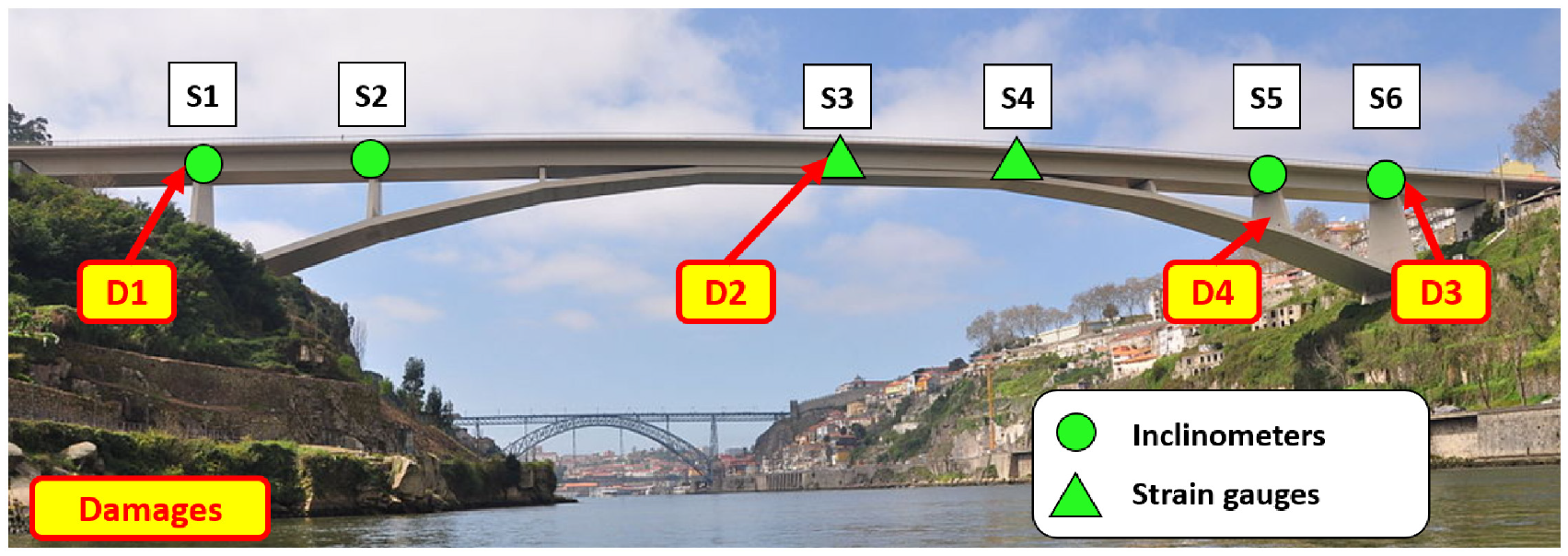
Instrumented sections with local variables and damage locations.
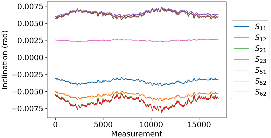
Evolution of the seven inclinometers over the monitoring period.
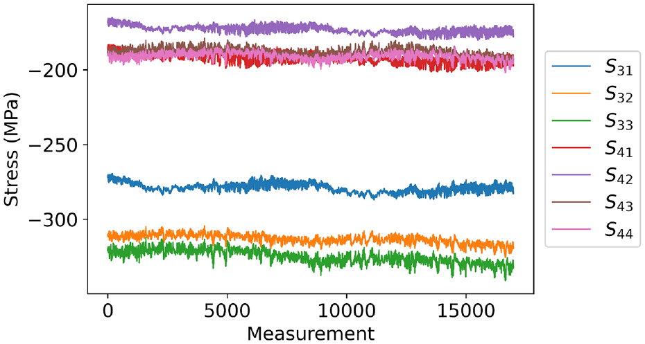
Evolution of the seven strain gauges over the monitoring period.
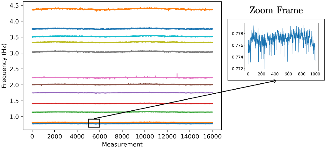
Evolution of the first 12 eigenfrequencies over the monitoring period. The squared window represents a subset of 1000 measurements of the first eigenfrequency to show the variability over time.
Statistical properties of the long-term eigenfrequency data.
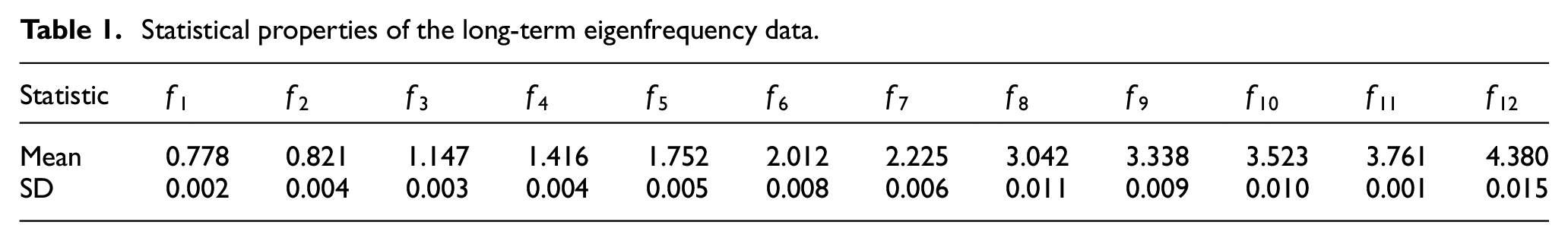
Since the local variables yield one measurement per hour while eigenfrequencies are produced every half an hour, we compute the mean of every two eigenfrequency measurements to use data from both monitoring systems with a time resolution of 1 h. After removing null values, a total of 16,005 measurements is obtained for each variable. From these data, the first
DNN approach
We employ a data-driven method based on autoencoder DNNs. We intend to exploit the advantages of combining multiple sources of monitoring data in the task of damage detection. The architecture follows the scheme developed in our previous work. 81 It provides adequate results according to the results obtained in Fernandez-Navamuel et al. 81 However, there may exist other architectures that provide adequate results as well. Optimizing the architecture compared to other existing approaches is out of the scope of this work.
The architecture contains two adding blocks at the encoder and the decoder stages, namely a linear and a nonlinear one. Its main advantage lies in allowing to employ a simple linear architecture (analogous to PCA), which accelerates the training phase over deeper architectures. 7 Besides, this strategy enhances the explainability of the neural network, since the contribution of nonlinear transformations can be explicitly separated from the linear ones. 7 Figure 5 shows the block-wise architecture of the autoencoder.
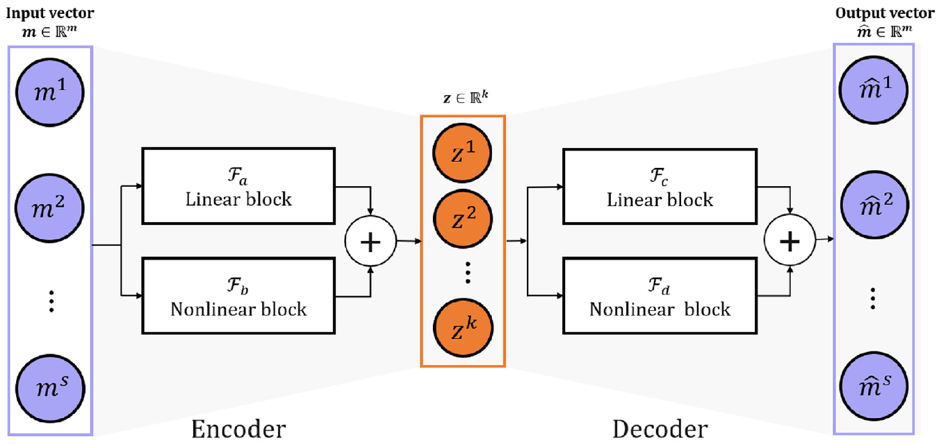
Block diagram of the autoencoder with parallel connections.
Let
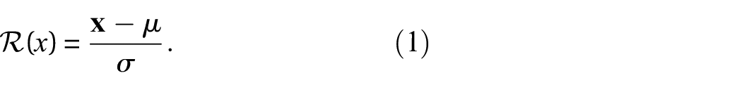
The rescaled measurements are obtained as

Here,

where

where
The optimal parameter set
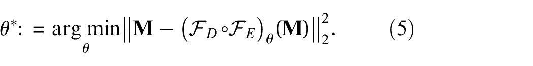
The final goal of the autoencoder is to detect abnormal responses in the structure from the value of the reconstruction error. If damage alters the structural response, the latent representation
The three DNNs follow the scheme sketched in Figure 5. All the architectures are fully connected with only dense layers. The linear encoder
The architectures of
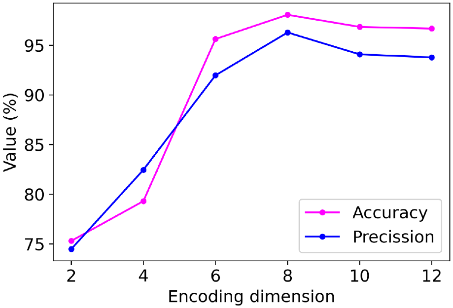
Sensitivity analysis of encoding dimension on accuracy and precision metrics.
The proposed architectures provided adequate results while avoiding overfitting problems. Other architectures could be employed, but optimizing the architectures is out of the scope of this work.
86
The hyperparameter selection found in previous studies on gradient-based training of DNNs.87,88 We employ Adam optimizer given its ability to prevent getting trapped in local minima.
89
A small learning rate may result in slow training and, in some cases, getting stacked in a local minimum.
90
Contrarily, a significant learning rate may cause instability during training or even divergence of the loss function.
91
In this work, a learning rate of
Summary of architecture and training specifications.
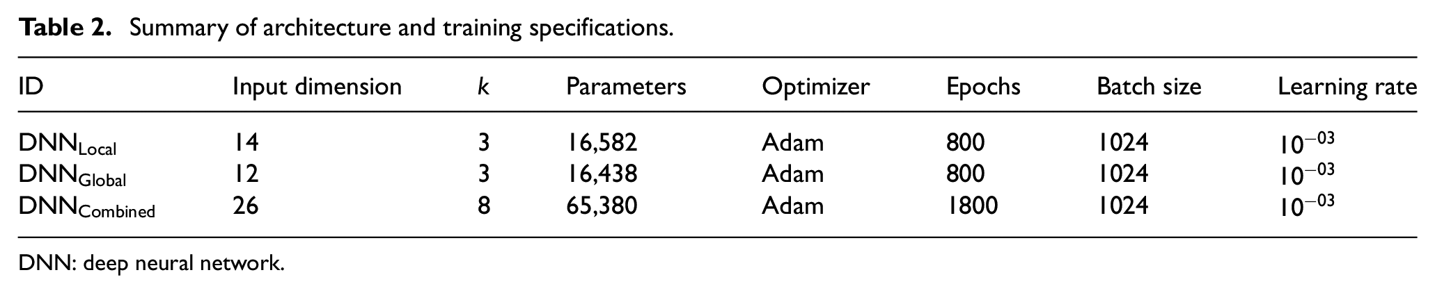
DNN: deep neural network.
The networks are trained and validated with long-term monitoring data corresponding to the healthy state of the bridge (unsupervised learning). This period covers 2 years of environmental and operational variability. New (unseen) measurements corresponding to the healthy state are expected to produce a feature vector
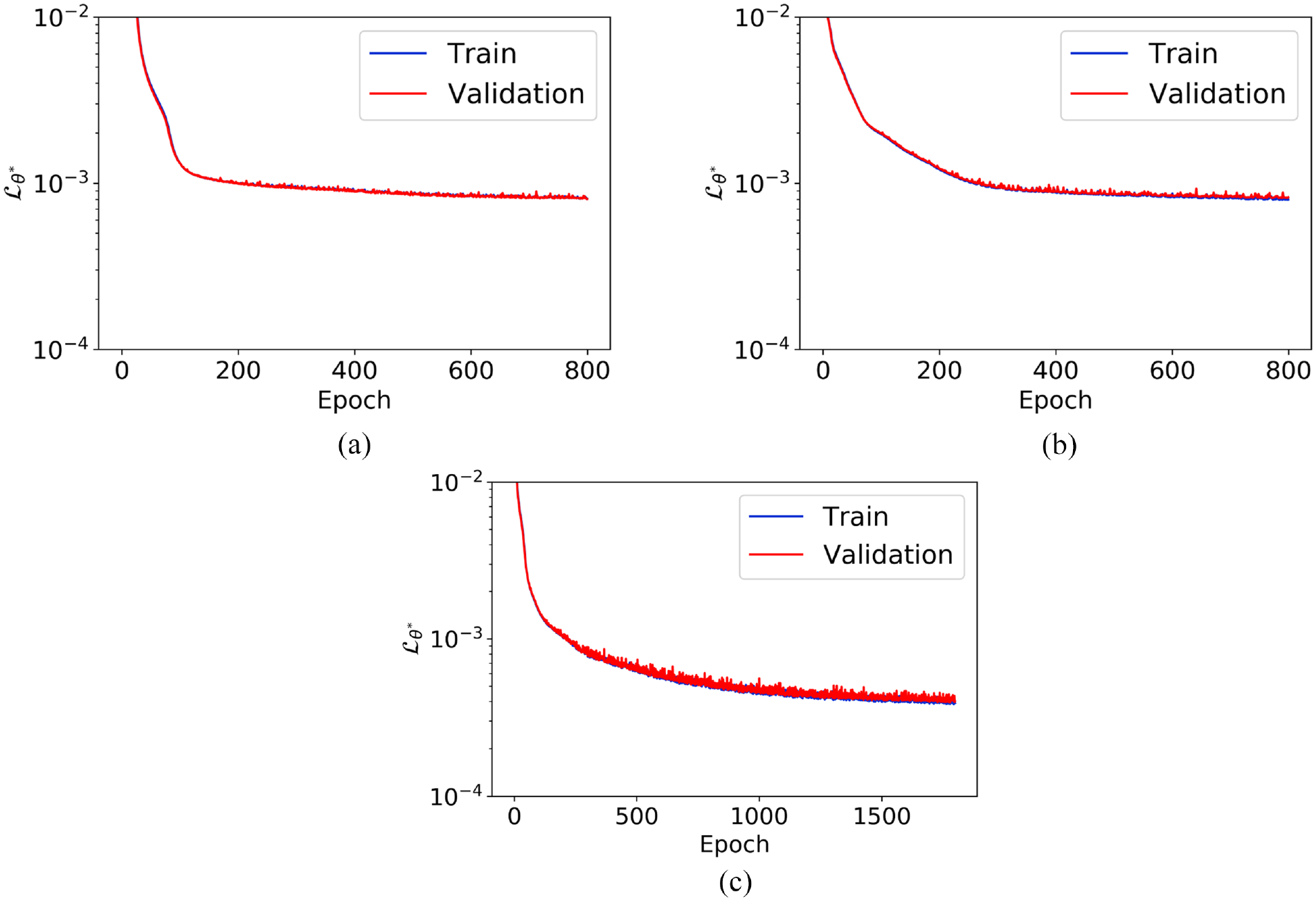
Loss evolution of the designed DNNs: (a) loss evolution for
Simulation of damage for testing
Once the autoencoder is trained to reconstruct healthy monitoring data under varying EOCs, we must test its performance under new unseen scenarios, including damage. From the available long-term monitoring data,
Damaged scenarios
Let us assume that the target structure, under specific EOCs, has an undamaged response
However, since the damaged response is unavailable experimentally, we employ a FE model that represents the structural behavior. The model is built in ANSYS® using 3D elastic beam-type (BEAM4) elements. It is an uniaxial element that allows tension, compression, torsion, and bending. Figure 8 shows an extruded view of the FE model (not the real geometry of the cross-sections).
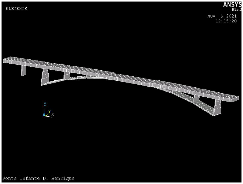
Extruded view of the FE model built in ANSYS®.
The FE model is built based on engineering knowledge and prior information but includes simplifications and assumptions that make its response differ from that of the true structure.
84
In order to reduce that discrepancy, the model undergoes an updating process to match the response measured during an ambient vibration test with specific EOCs. This approach is a standard practice in the scientific community since a denser sensor array is deployed during the ambient vibration test compared to long-term instrumentation, allowing to characterize the shape of the eigenmodes with higher resolution. The updating process is fully described in Magalhães et al.,
84
where the relative errors with respect to the dynamic response in the ambient vibration test were calculated. Table 3 summarizes the updating results and compares the numerical response of the final model with the ambient vibration test, revealing errors below
Model updating results obtained by Magalhães et al. 84
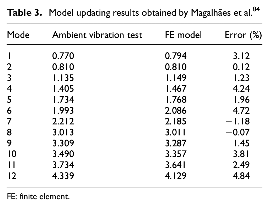
FE: finite element.
Accurately simulating damage demands a substantial computational effort and human expertise. These resources could be unavailable or unprofitable, and simpler approximations are needed. In this work, damage is feasibly simulated by reducing the inertial properties to represent a loss of vertical bending stiffness at small-length segments of the structure. When simulating damage, we employ BEAM4 elements, which directly modify the inertial properties and preserve the mass value (fixed area and material). In these elements, the flexural inertia for the vertical bending can be reduced by affecting the corresponding real constant of the element, that is, without affecting the mass, material properties or other inertial properties of the bridge. For that purpose, we first alter the geometry in separate cross-section models to achieve the flexural intertia value corresponding to the damage level. The geometrical modification consists of slightly reducing the bottom slab height. Magalhaes et al.
93
provide descriptive information of these geometries. Figure 9 shows the geometry modification introduced at

Comparison of the original and modified geometry at
We then introduce the new (damaged) intertia value into the BEAM4 elements of the affected sections of the bridge FE model. It was first proposed and applied to the same bridge by Magalhães and Cunha
73
to reproduce possible consequences of aging phenomena, corrosion, or extreme events. The same damage scenarios were also employed for validation in our previous work.
81
Other works, such as,94,95 also employ stiffness reductions to reproduce damage scenarios, considering reduction levels up to
Vertical bending inertia reductions for damage D2.
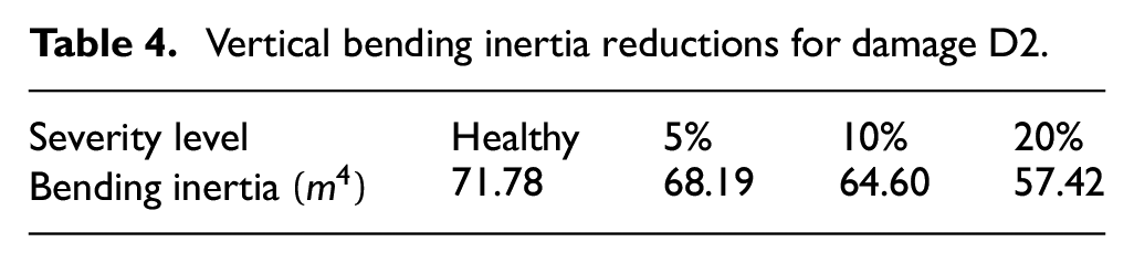
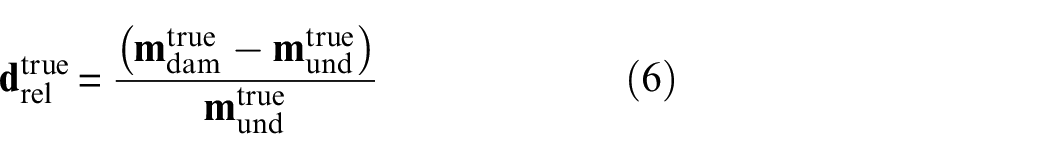
Analogous to Equation (6), we calculate the relative differences between the undamaged and the damaged responses for the FE model as:
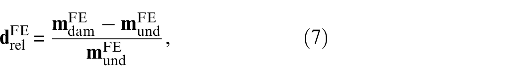
where
Relative differences
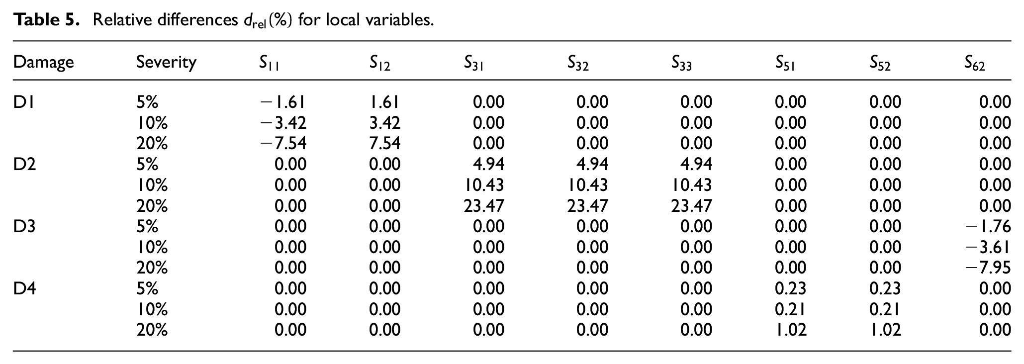
Relative differences
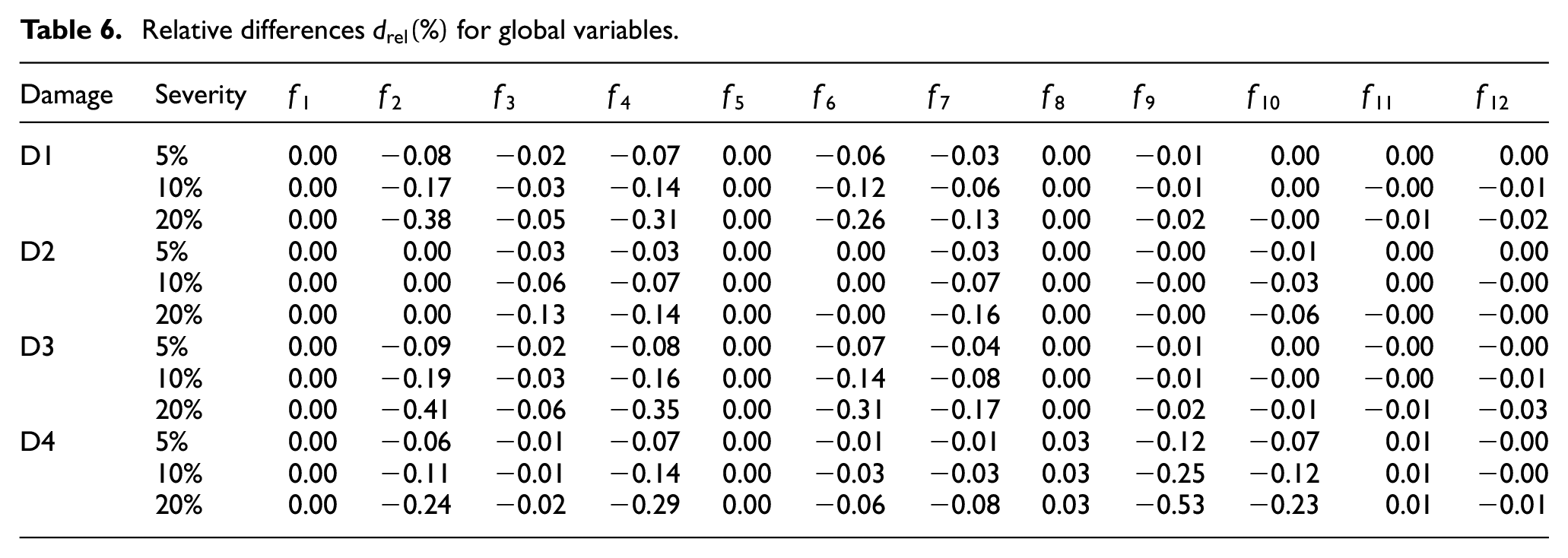
Given the impossibility to obtain

In this work, we assume that modeling error affects the structural response differently than damage and, thus, that the shift due to modeling error will not overlap with the shift produced by damage. Figure 10 schematically represents this assumption. With this assumption, the minimum detectable damage depends on the sensitivity of the response and not on the modeling error.
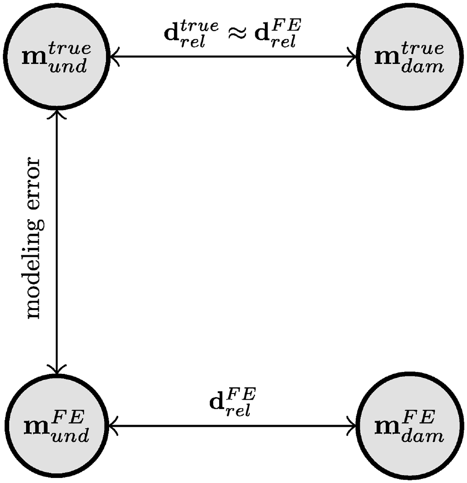
Schematic representation of modeling error and damage-induced changes.
Damaged datasets
The proposed FE simulations disregard the effect of environmental and operational variability. Since the monitoring system provides one observation per hour, running time-domain simulations becomes unfeasible to generate a representative dataset for evaluating the proposed methodology. This modeling scope poses a limitation to the proposed methodology since the change between the healthy and the damaged responses (Equation (6)) may slightly change under varying EOCs. However, it is believed that this second-order phenomenon barely influences the ratio and can be neglected, as supported, for example, in Magalhães 6 and Comanducci et al. 26
In order to incorporate the effect of EOCs in the testing phase, we apply Equation (8) to the measurements in the monitoring subset preserved for testing. These measurements are subject to the effect of varying EOCs unseen during training and thus incorporate this variability during the testing phase. We assume that the damage evolves slowly enough to consider that it remains constant during the testing period. We build 12 damaged datasets (one for each scenario and severity level). The healthy testing dataset contains
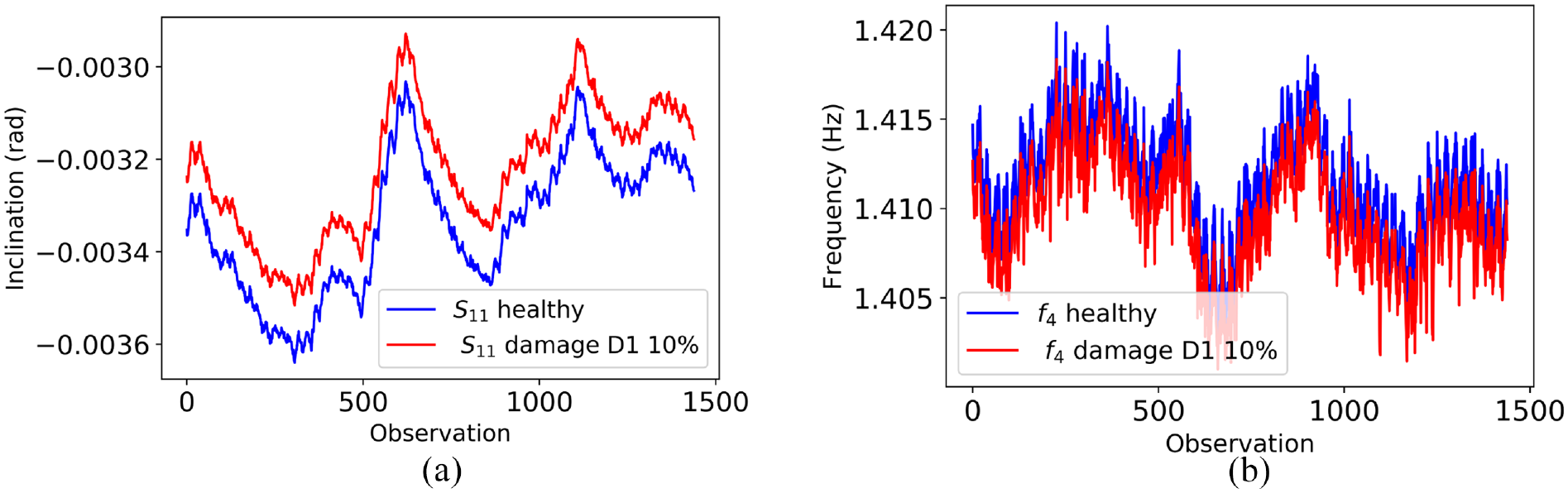
Effect of damage D1 with 10% severity on: (a) effect of damage D1 with 10% severity on
Results
Damage detection
As introduced in section “Deep neural network approach,” the reconstruction error
In the context of SHM, a false positive indicates healthy data misclassified as damage, and a true positive indicates a correctly classified damaged scenario. Unsupervised learning results in a single-class classification, where undamaged data belong to the healthy class and any damaged scenario corresponds to an outlier.
96
The detection ability consists of classifying new unseen healthy observations as undamaged and detecting any departure as an outlier. False-positive and true-positive rates are obtained according to a threshold value
Let
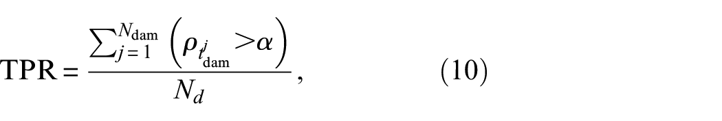
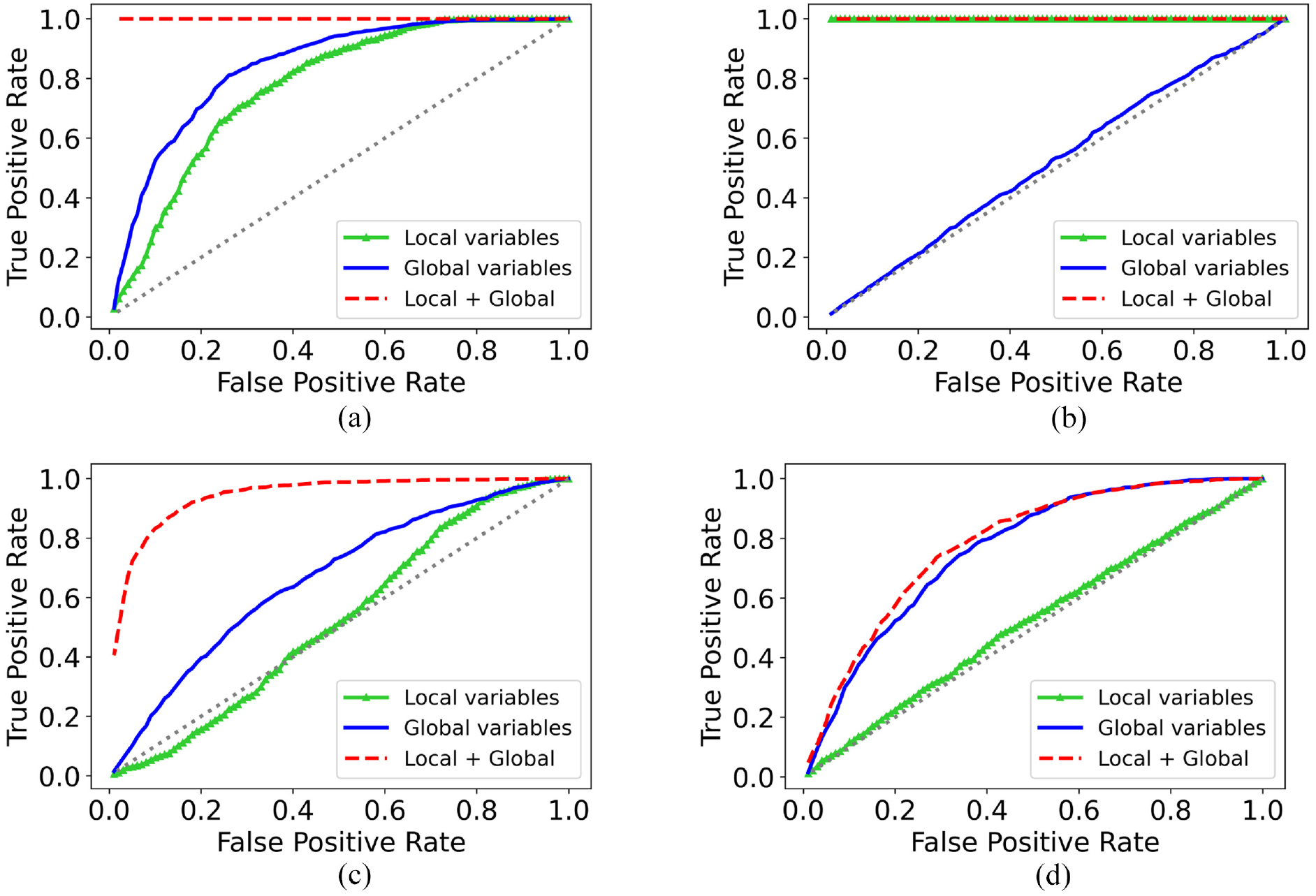
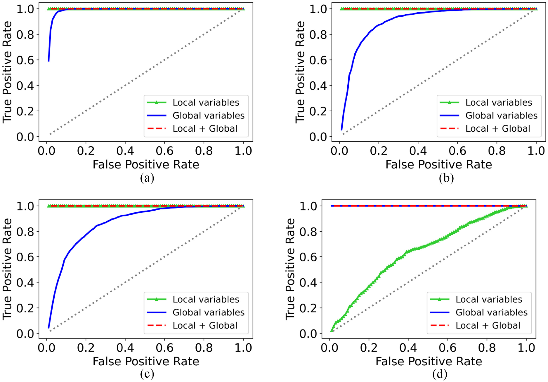
Figures 12 to 14 compare the performance of the three designed DNNs for each type of damage to demonstrate the benefit of combining local and global variables. In the figures, the random classifier is represented with a grey dashed line. The performance increases as the curve moves away from the grey line and approximates the top of the ROC space.
ROC curves for damage severity 5%: (a) damage D1 5% severity, (b) damage D2 5% severity, (c) damage D3 5% severity and (d) damage D4 5% severity.
ROC curves for damage severity 10%: (a) damage D1 10% severity, (b) damage D2 10% severity, (c) damage D3 10% severity and (d) damage D4 10% severity.
ROC curves for damage severity 20%: (a) damage D1 20% severity, (b) damage D2 20% severity, (c) damage D3 20% severity and (d) damage D4 20% severity.
Local variables exhibit good performance for damage scenarios D1–D3, mainly for severity levels above
Given the limited sensitivity to damage severity of
Performance metrics for damage severity
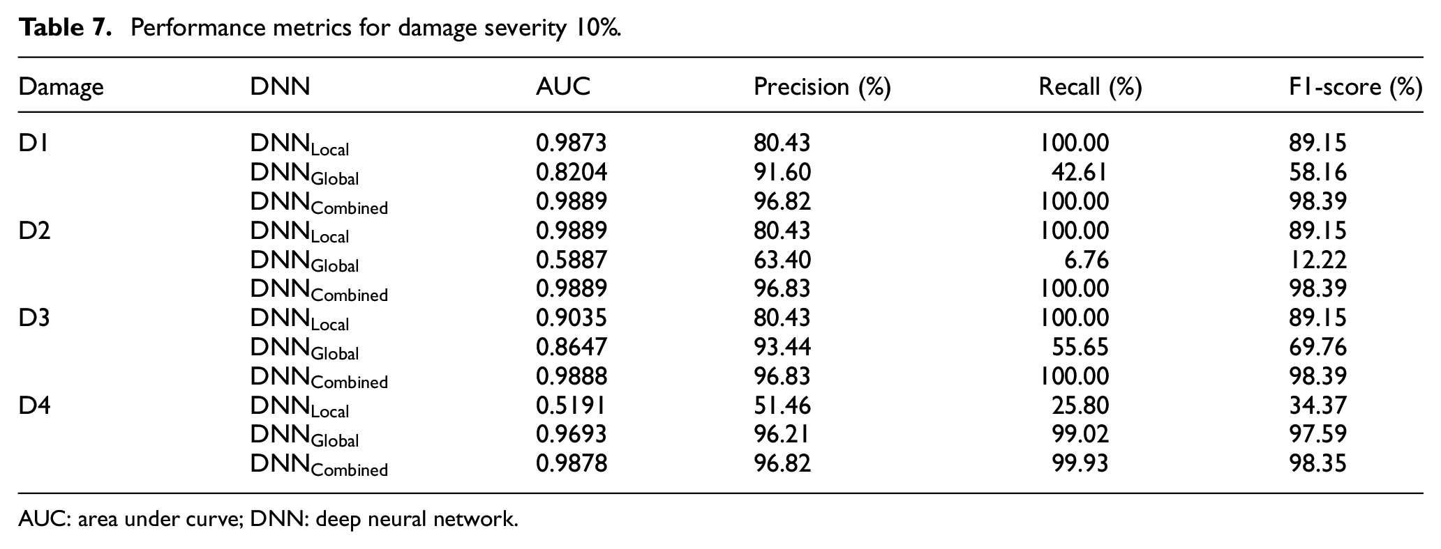
AUC: area under curve; DNN: deep neural network.
We also explore the latent space for each damage scenario. Figure 15 compares the latent space representation of local variables for a
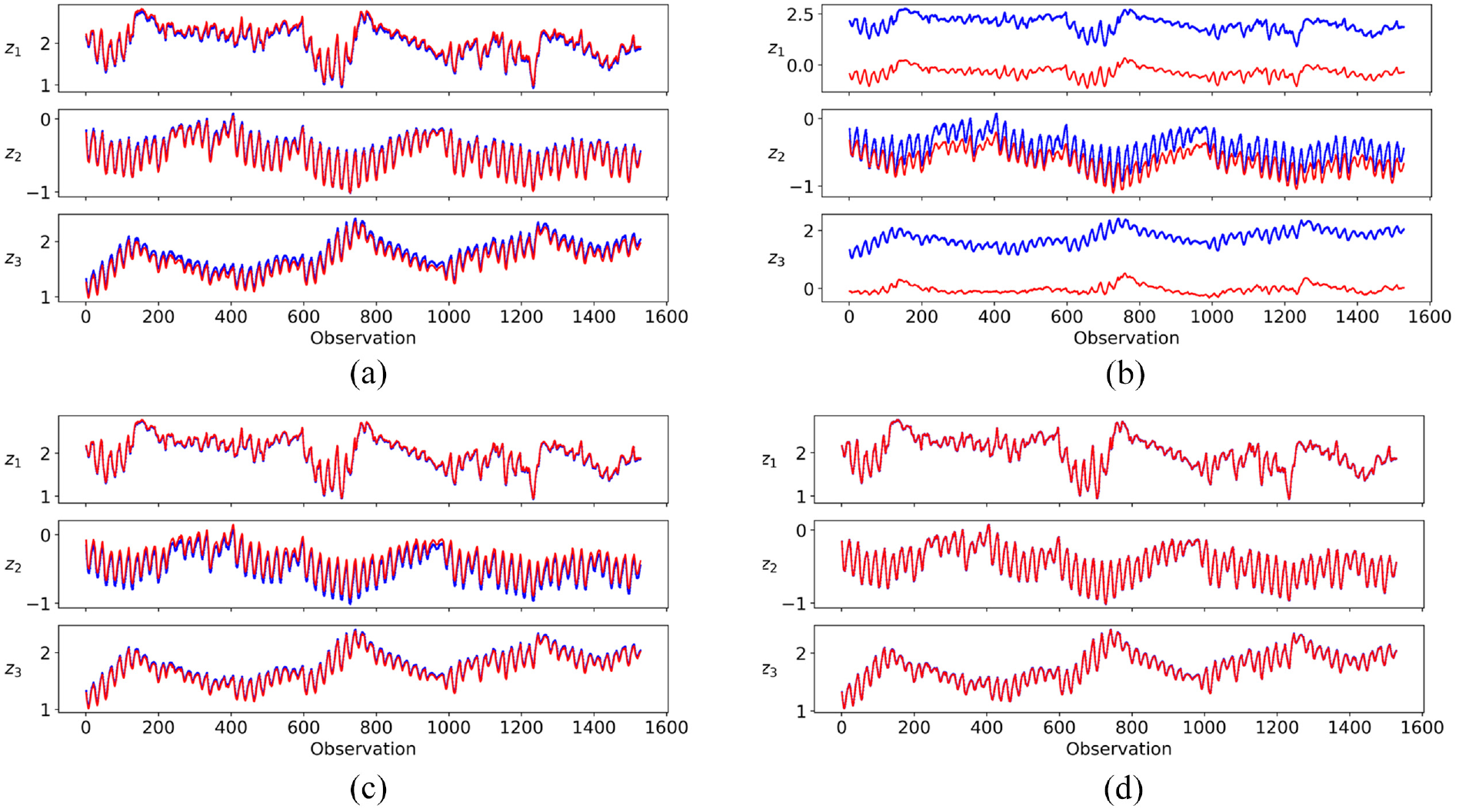
Comparison of the healthy (blue) and damaged (red) 3-dimensional latent space for
On the other hand, global variables adequately detect the four damage scenarios when the severity reaches
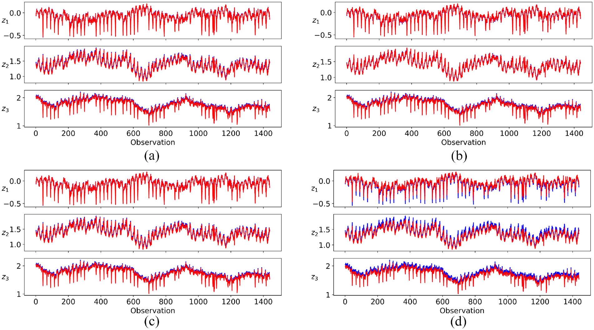
Comparison of the healthy (blue) and damaged (red) 3-dimensional latent space for
Since damage was introduced as a vertical stiffness reduction, it mainly affects the vertical bending eigenmodes. In this case, only four out of the 12 global variables represent vertical bending eigenmodes and thus participate in detecting the proposed damage scenarios. The rest of the mode shapes are lateral and torsional. Figure 17 shows the four vertical bending mode shapes adopted in this work. For damage cases D1–D3, (occuring at the deck of the bridge), damage D2 presents practically null curvature, yielding the worst results. Damage D2 occurs in the middle deck (see Figure 1) and it slightly affects global variables due to the low curvature of the involved eigenmodes at this position (see mainly Figure 17(a) and (d)). Hence, although global variables increase the range of detectable damage compared to local variables alone, they still present some limitations, mainly for reduced severity levels. It is worth noting that
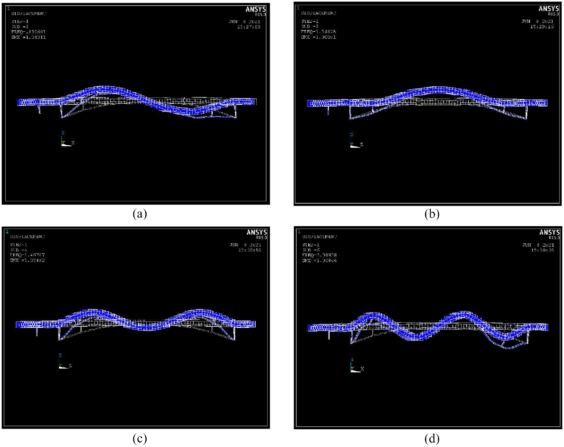
Vertical bending eigenmodes: (a) first vertical eigenmode, (b) second vertical eigenmode, (c) third vertical eigenmode and (d) fourth vertical eigenmode.
In light of the previous observations, it becomes interesting to combine both sources of monitoring data. The red dashed line in Figures 12 to 14 reveals that combining local and global variables outperforms the classification ability of local or global variables alone. The ROC curves denote a multiplicative enhancement of the results that goes beyond the sum of the individual contributions of local and global variables. This becomes more evident mainly for lighter damages (see, e.g., Figure 12(c)). In the case of damage D4, since the contribution of local variables is very low (see, e.g., Figure 14(d)), the combined solution practically coincides with the performance of global variables only. Figure 18 compares the 8-dimensional latent space representations of the damage scenarios (
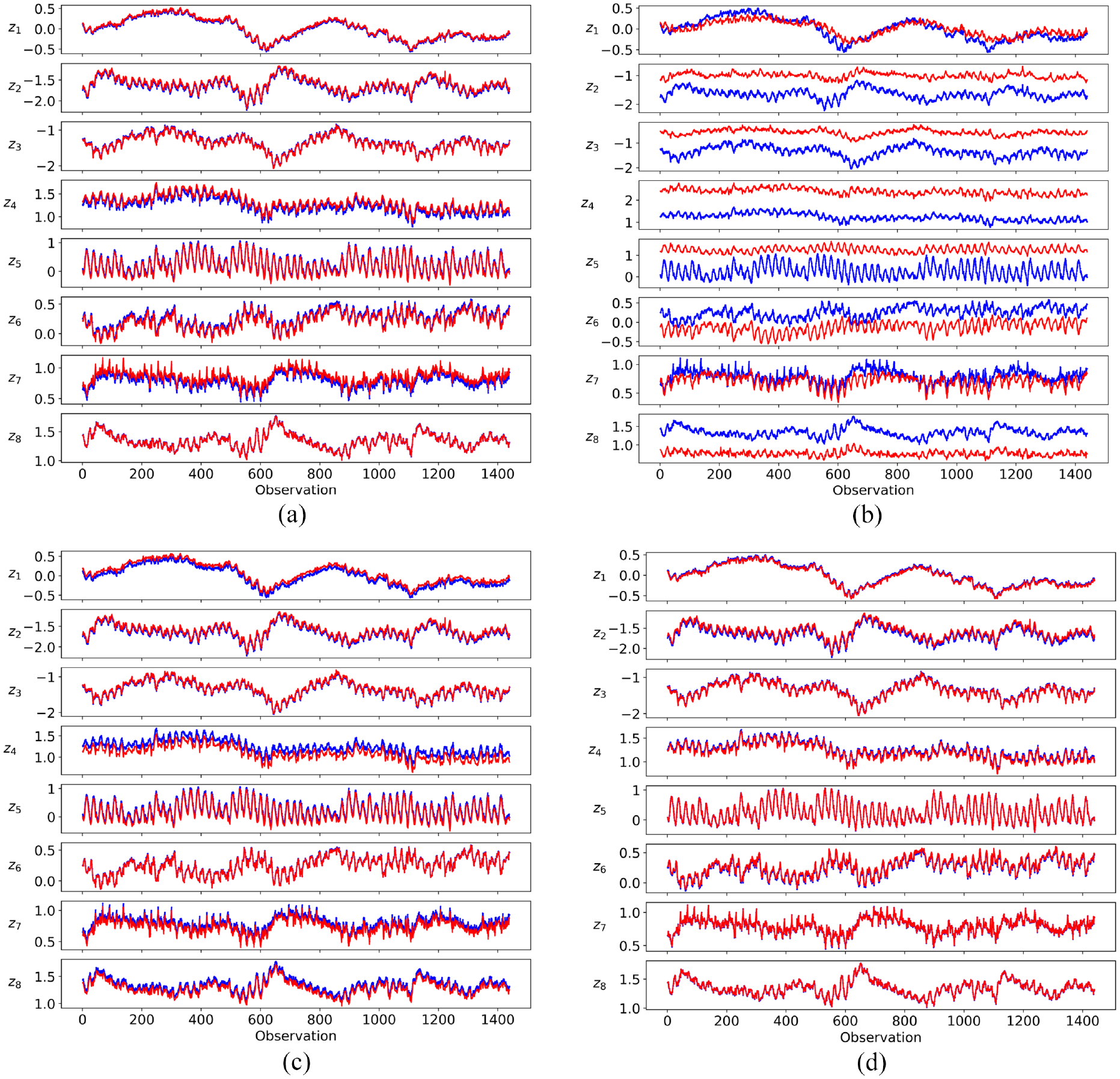
Comparison of the healthy (blue) and damaged (red) eight-dimensional latent space during testing: (a) damage D1 with 10% severity, (b) damage D2 with 10% severity, (c) damage D3 with 10% severity and (d) damage D4 with 10% severity.
In general, the obtained ROC curves for the combined approach are very good for severity levels of
Damage location
In addition to detecting damage occurring nearby the sensor emplacement, local variables also contribute to determining the damage location. It is expected that the autoencoder yields an outlier (
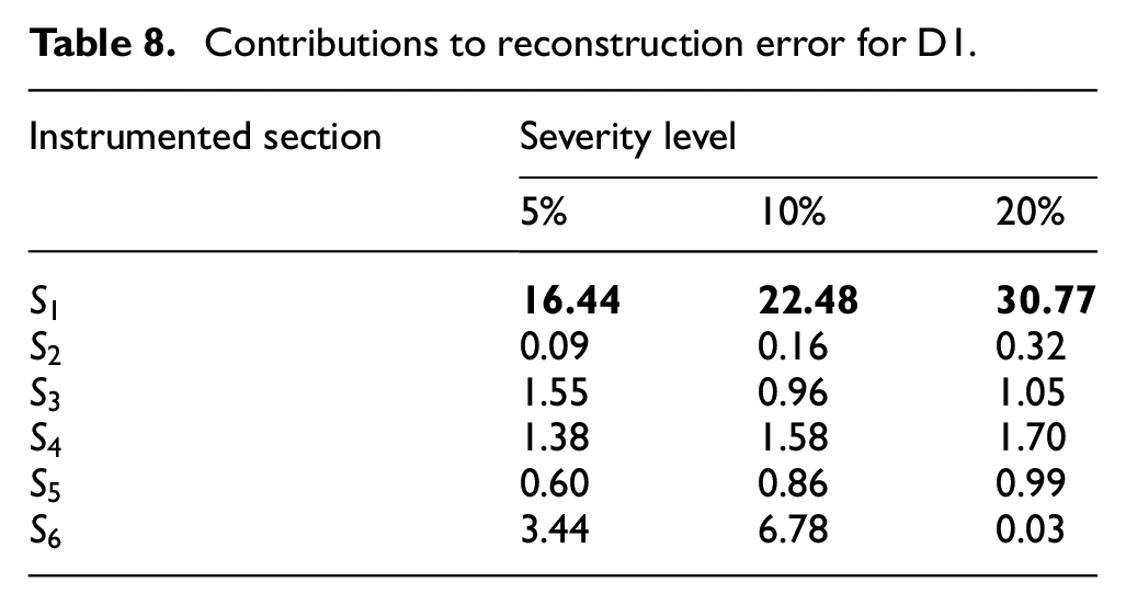
It is assumed that if damage occurs nearby an instrumented section, it will mainly affect the corresponding local variables, and the autoencoder will reconstruct these variables more deficiently. Hence, the highest contribution to the reconstruction error would result from variables measured with the sensors located nearby the damaged region. Here, the reconstruction error of local variables is analyzed using the combined autoencoder (
Contributions to reconstruction error for D1.
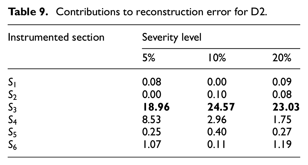
Contributions to reconstruction error for D2.
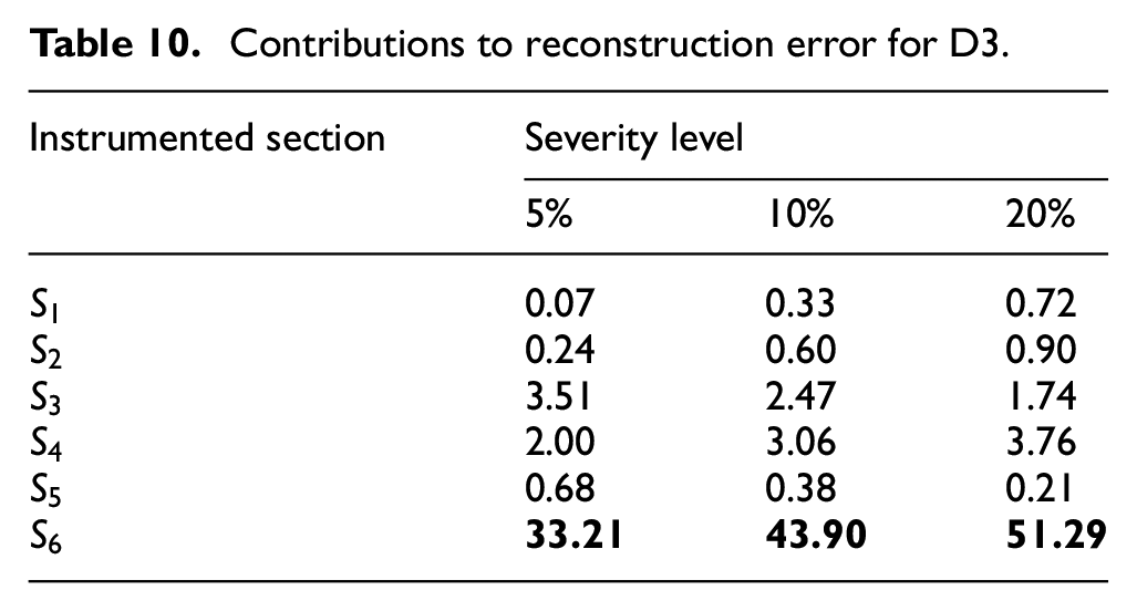
Contributions to reconstruction error for D3.
Contributions to reconstruction error for D4.
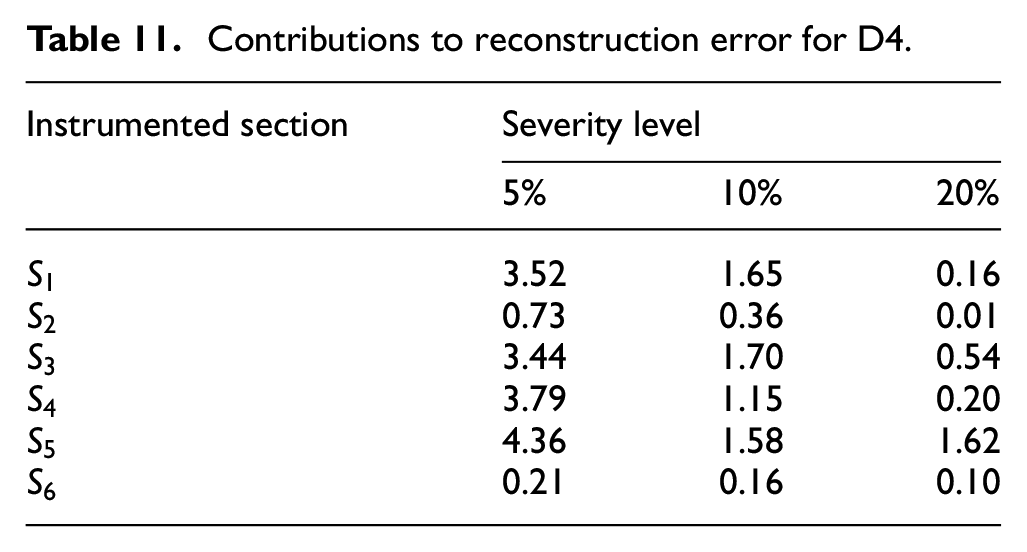
Results demonstrate that damage D1–D3, which occur close to instrumented sections that measure local variables, are adequately located even for reduced severity levels (see Tables 8 to 10). The contribution of the affected section is considerably higher than those of the rest of the instrumented sections. By contrast, local variables are unable to inform about the location of D4, since no local variables are recorded close to it. This means that local variables only aid to locate damage occurring close to their emplacement.
SHM strategy
The final goal of the methodology is to detect abnormal behavior of Infante Dom Henrique bridge during operation from experimental monitoring data. Given the successful results observed in section “Results,” we employ the combination of local and global variables as the input data and thus employ the corresponding DNN (
We employ the cumulative error after five measurements to reduce the risk of occurrence of false positives and produce a more robust alert system.
6
This means that the detection time is 5 h, since the monitoring system provides one observation per hour including the measurements of the local and global variables. The threshold value
Damage detection
Figure 19 shows the control chart of the reconstruction error. The logarithmic scale is applied to the reconstruction errors to better visualize the results. The grey-shadowed region indicates the part of the testing with damage, and the vertical dashed lines delimit the subset associated with each damage. Measurements exceeding the threshold value (blue horizontal line) are red-colored, and those below the threshold are green-colored. The figure reveals that undamaged measurements are properly classified as healthy, with a
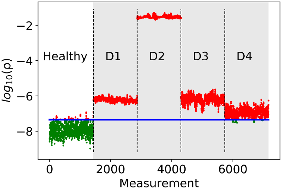
Testing control chart with damage severity of
Damage location
We finally analyze the four damaged testing datasets to explore/investigate the ability of the method in damage location. We obtain the contribution to the reconstruction error at each section instrumented with local variable sensors (
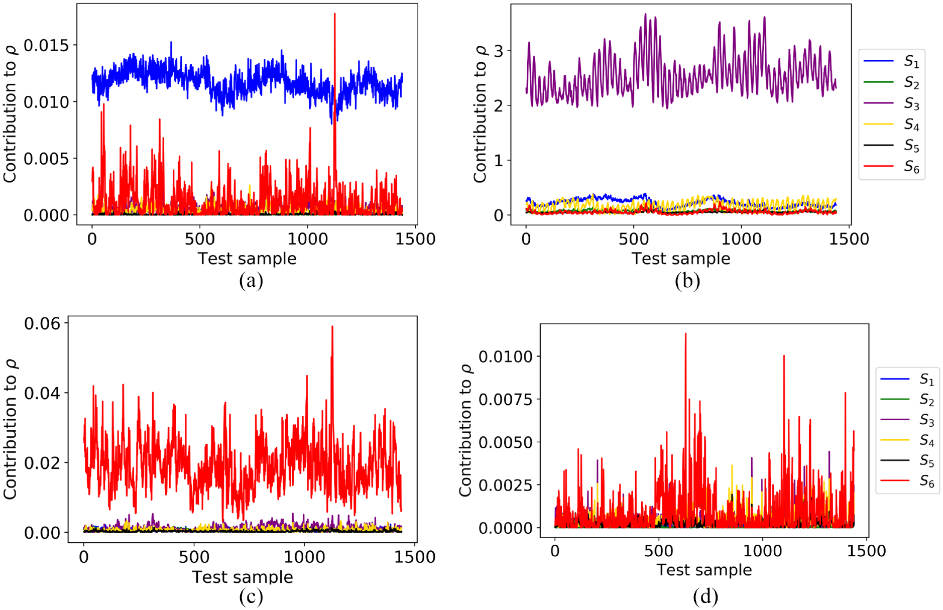
Contribution of local variables to the reconstrution error in presence of damage: (a) local variable contributions to
Conclusion
An unsupervised learning approach was developed and tested to detect damage at the Infante Dom Henrique bridge in Porto. A particular DNN based on an autoencoder with two adding blocks at the encoder and decoder was employed to account for nonlinear relationships. The reconstruction error, which measures the discrepancy between original and predicted measurements, is the damage-sensitive feature for outlier detection. Reaching a higher identification level (quantification and location) requires adopting a supervised learning strategy where simulated damaged data participates in the training phase of the data-driven model, which is a topic of interest to our research. Three DNN architectures were created to accommodate different inputs and investigate the potential of combining measurements from various sensor types, namely, local and global variables. The testing phase included healthy and damaged measurements to produce the ROC curves. The damage was simulated using a FE model of the structure by reducing the vertical bending stiffness to produce the relative change between the healthy and damaged responses. This relative shift affected a portion of the monitoring data preserved for testing purposes, subject to environmental and operational variability.
The classification performance of local, global, and a combination of both variables was compared and examined by analyzing the resulting ROC curves and the latent space representation. Some standard metrics (AUC, precision, recall, and F1-score) evaluated the classification performance. Results revealed that local variables successfully detect damage occurring nearby the sensor emplacement but strongly fail for distant damage, such as D4, which practically yields a random classifier. Global variables enlarge the detectable space but with limited sensitivity for slight severity levels. Besides, they still present some gaps at locations where the associated eigenmodes have a small curvature that restricts the sensitivity of the corresponding eigenfrequency. It is the case of damage D2, which provides a low-performance classification.
After analyzing the combination of variables, an enhancement in the detection ability of the reconstruction error was observed, allowing us to detect lighter severity levels. When damage occurs far from local variables, the combined DNN reaches only the same solution as global variables alone since there is no contribution from local variables. Results reflect the enhancement attained when combining both data sources in terms of damage sensitivity.
We also investigated the ability of local variables to inform about the location of damage. By calculating the contribution of local variables at each instrumented section to the total reconstruction error, we attained that local variables successfully locate damage that occurs in the vicinity of the sensor emplacement. We concluded that local variables aid in the detection task and contribute to finding the possible damage location. However, the method is unable to locate damage when it occurs far from instrumented sections, which poses a limitation to the approach in locating damage.
Results suggested that an important issue when implementing SHM systems lies in the adequate disposal of the sensors. Deploying many sensors helps to improve diagnostics, but it results in inadmissible costs. An intelligent positioning strategy might yield a more efficient solution. Essential locations are, apart from those more susceptible to suffering damage (e.g., joints, pier foundations), those where eigenmodes present small curvature values since global variables lose sensitivity at these positions. Since eigenmodes can be obtained beforehand (through an ambient vibration test or numerical simulations), those nodes that are more “blind” to global variables can be identified and supported with local variable sensors.
The proposed method presents some modeling limitations that must be mentioned and addressed. The employed FE model is subject to assumptions and simplifications that introduce a discrepancy with respect to the true structural response. Although we overcome this discrepancy by tuning the boundary conditions in the model, a more sophisticated method based on iterative updating could provide more accurate results. Besides, the employed FE model disregards the effect of varying EOCs since it is updated for the specific EOCs occurring during an ambient vibration test. We consider future work incorporating EOCs in the damage simulations to obtain more realistic shifts between healthy and damaged scenarios. Using bayesian approaches both in the updating process and in the autoencoder architecture contributes to handling these variability sources mainly when combining numerical simulations with experimental data, posing a key topic for our future developments.
We also consider as future research the investigation of other damage scenarios to extend the validation of the proposed methodology and to demonstrate the potential of monitoring data in the early assessment of the structural behavior of bridges. Representing degradation phenomena in the system or subcomponents to identify performance trends and prevent catastrophic failures poses a future study of interest focused on predictive maintenance.
Finally, in line with our previous works on supervised learning,99,100 we also contemplate as future work investigating the discrepancy between the experimental and numerical healthy state and its effect in the damage identification task. We will explore domain adaptation techniques to minimize the distance between both spaces and accurately classify damage location and severity.
Footnotes
Appendix A
This appendix reports some comparisons of different DNN architectures. We provide this material to demonstrate that combining local and global variables brings an important enhancement in the damage detection task regardless of the selected architecture.
We first explore sequential, fully connected DNNs without parallel connections. We design three dense architectures, one for each dataset. We use the same layers as those in the nonlinear blocks in our proposed architectures. Table A1 provides the number of parameters for each DNN. We consider the four damage scenarios with a
In the considered DNNs, the architectures designed for the combined dataset require a much larger number of parameters compared to local and global datasets. This parameter increase occurs since we unavoidably must modify the input and output layer dimensions to accommodate the different input sizes. Besides, the the hidden layers must be redimensioned accordingly. Although these are the minimal adjustments to adapt the input data, they may result in very different architectures that make it challenging to fairly compare the three datasets. For this purpose, we explore two types of similarity in the architectures.
Figure A3 depicts the new ROC curves with the modified architectures. Although the three DNNs are now comparable in terms of size, such a big increase in the number of parameters of
Acknowledgements
The collaboration of Engineer Renato Bastos and Kinesia in the sharing of Infante D. Henrique Bridge data are deeply acknowledged.
Declaration of conflicting interests
The author(s) declared no potential conflicts of interest with respect to the research, authorship, and/or publication of this article.
Funding
The author(s) disclosed receipt of the following financial support for the research, authorship, and/or publication of this article: This work was financially supported by: Base Funding – UIDB/04708/2020 of the CONSTRUCT – Instituto de I&D em Estruturas e Construções – funded by national funds through the FCT/MCTES (PIDDAC). David Pardo has received funding from: the Spanish Ministry of Science and Innovation projects with references TED2021-132783B-I00, PID2019-108111RB-I00 (FEDER/AEI) and PDC2021-121093-I00 (MCIN/AEI/10.13039/501100011033/Next Generation EU), the “BCAM Severo Ochoa” accreditation of excellence CEX2021-001142-S/MICIN/AEI/10.13039/501100011033; the Spanish Ministry of Economic and Digital Transformation with Misiones Project IA4TES (MIA.2021.M04.008/NextGenerationEU PRTR); and the Basque Government through the BERC 2022-2025 program, the Elkartek project SIGZE (KK-2021/00095), and the Consolidated Research Group MATHMODE (IT1456-22) given by the Department of Education. Authors would like to acknowledge the Basque Government funding within the HAZITEK programme (ERROTAID project) and TCRINI project (KK-2023-0029), and the European Horizon (HE) with LIASON project (GA 101103698), and FUTURAL project (101083958).