
Abstract
Population-based structural health monitoring (PBSHM) expands structural health monitoring (SHM) from a single structure to a group of structures, allowing inferences to be made within and between populations by transferring knowledge across them. Within the populations of interest, the similarity of structures, via their corresponding data, should be assessed to successfully implement PBSHM. This paper focusses on using distance metrics to assess similarity at the very start of the analysis chain, to discover information about a population for which there is little prior knowledge and before any analysis has taken place on individual structures. By doing so, it is possible to quickly and automatically identify abnormalities within the population, group similarly behaving structures together, and inform further decisions. The suitability of several candidate metrics that are not widely employed in SHM are tested using a number of commonly occurring feature behaviours, such as varying amplitudes and temporary mean shifts. The effect of data normalisation/standardisation on the metrics is also explored to identify interesting behaviours within the data. A case study is then presented where distance metrics are used to discover similarities and dissimilarities within temperature data from turbines in an offshore wind farm.
Introduction
In civil and aerospace structures such as bridges and wind turbines, the presence of damage can be costly; damage can lead to failures that cause expensive downtimes, or in extreme cases, put lives at risk. Understandably, developing methods to identify damage and predict its progression is immensely important in order to avoid catastrophic failures. In general, current techniques address these tasks via regular manual inspections and expert engineering knowledge, which is time consuming and expensive to undertake. Structural health monitoring (SHM), seeks to detect and diagnose damage automatically from monitoring data collected from structures, reducing the manual burden on owners. The aim of SHM is to reduce unnecessary regular inspections and gain insights and predict behaviours using data and model-based methods. Ideally, this task would be formed as a supervised learning problem, where models are trained on damage-state labelled data. However, this necessitates measurements of a structure in different possible damage states, which may include multiple-site and multiple types of damage. In reality, it is rare that monitoring data are available from structures in any of their damage states; typically, measurement systems that capture damage are rare, defects are usually repaired prior to damage to reduce risk to users, and, more importantly, data from a single structure is unlikely to contain all types of damage it can possibly experience – resulting in a training phase of the SHM model that will not generalise in the testing phase. Consequently, focussing on single structures in a standard SHM setting can give a limited view of the variety of damage that is possible. Population-based structural health monitoring (PBSHM),1–8 aims to address this shortcoming by studying entire groups of structures simultaneously, thereby increasing the knowledge-base of structural behaviours and damage states. Interestingly, the population of structures here can be homogeneous (structures within the population are nominally identical) or heterogeneous.
One of the forerunning technologies that aid PBSHM in achieving health-state inference across populations is transfer learning. 9 Transfer learning aims to improve the performance on target domains by leveraging information from related source domains. In the context of PBSHM, the target domain contains structures with incomplete data (such as missing/lack of damage labels), and the source domain contains structures with labelled data. For transfer learning, similarity between domains is a key factor. Dissimilar domains can lead to a phenomenon named negative transfer, 9 where the performance in the target is negatively affected by leveraging information from a source domain, that is, the performance is worse as a result of transfer than using just target data in the model. Therefore, to infer health states of one structure by studying a population of others, there is a clear need to determine similarity within populations, in order to identify and group similarly behaving structures.6,10 Similarity, as it happens, is also an important consideration in standard supervised SHM methods, because unexpected disparities between training and testing data can lead to reduced model performances during testing.
In PBSHM, similarity can be measured at two levels: structural similarity and feature similarity. The hypothesis here is that feature data collected from structures is best suited for transfer learning if the structures are similar in their composition. Results from a recent study on PBSHM supports this hypothesis.2,11 Structural similarity considers the dynamic behaviour of structures based on their construction and boundary conditions. By representing structures as attributed graphs, similarity of structures can be measured.2,12 The converse hypothesis to the aforementioned ‘similarity in structure implies similarity in data’, is ‘similarity in data implies similarity in structure’, 13 and the wish in PBSHM is to enable assessment of similarity in both cases (and eventually simultaneously). In this paper, the focus is on measuring similarity of monitoring data and descriptive features collected from structures. It is important to understand the behaviour of data during normal operating conditions, under environmental and operational variations (EOVs), and during deterioration and/or damage, in order to identify the most suitable data for transfer.
It is well understood that humans are experts in identifying changes or anomalies and recognising patterns in their surroundings. 14 Unfortunately, as populations grow in size and variety (vast sensor networks, multiple structures within homogenous and heterogeneous populations), manual analysis of large monitoring datasets becomes an impossibility. There is a need, therefore, to develop preliminary methods to identify similar and anomalous behaviours/trends in data quickly and automatically in a principled way, that forgo the need for time-consuming and in-depth analysis of individual datasets in a population. The intention is that this information may then be initially used to group structures together, highlight structures or components of the data that are performing differently from the majority of the population, etc., and inform further decisions such as, establish whether standard machine-learning approaches are appropriate across a population (i.e. find suitable training and testing data), and assess whether transfer learning is required.
There are many stages in a monitoring campaign where measuring similarity in features may be helpful. This paper focusses on methods that can be used at the very start of the analysis chain, to discover information about a population for which there is little prior knowledge and before any analysis has taken place on individual structures. Therefore, the methods suggested for assessing similarity in this paper do not speculate, infer, or aim to identify the condition of the structure (from which the data were collected), or the cause of any identified dissimilarities – whether the data are affected by interesting behaviours such as EOVs and damage, or whether they are a result of issues in the measurement chain (sensor damage, for example). Consequently, the underlying structure of the data could take any form, and the suggested methods of assessing similarity should be flexible enough to accommodate this.
To assess the similarity and to discover information about the data, the idea of a metric is employed here by treating the feature space (The feature space here is the space in which all features that correspond to each structure in a population lie)
This paper also considers the behaviour of features and metrics as the data are normalised/standardised, because it is a common pre-processing step in SHM18–20 and PBSHM.1,21 Dissimilarities in standardised data can indicate the presence of interesting behaviours (such as, higher-order moments). In PBSHM, standardisation helps bring source and target domains into the same space for domain adaptation. Methods such as normal condition alignment (that standardises and aligns data when structures are under normal operating condition) has proven incredibly useful for PBSHM in transferring knowledge across structures.22,23 Therefore, the behaviour of metrics as data are standardised is an important consideration for testing their effectiveness for PBSHM.
Original contributions
This is the first study that measures similarity of features across a population of structures to aid transfer learning in population-based SHM – a relatively new concept that aims to transfer information across groups of structures to increase the pool of available information, in order to increase performance of monitoring campaigns. Principled methods of assessing large amounts of engineering data quickly and automatically are necessary for PBSHM, although the methods suggested here can also help reduce analysis times for typical SHM steps such as identifying suitable training and testing data.
The study introduces distance metrics in the context of PBSHM, to automatically assess similarity between distributions of data which the authors argue are better suited to compare populations of structures (e.g. all wind turbines in a wind farm). Here, a survey of possibly useful distance metrics – that are not all widely used in SHM currently – is conducted to assess similarity of features in PBSHM.
The distance metrics are then tested against typical commonly occurring changes in data-sets and features that originate from SHM programmes. The responses of the metrics to the commonly occurring changes are mathematically formalised. The suitability and sensitivity of the chosen metrics to the feature changes in PBSHM are presented. The most appropriate candidate metric for a given feature behaviour is determined to aid fast and automatic similarity assessment.
The effect of data normalisation/standardisation on distance metrics is mathematically derived because it is a common analysis technique in domain adaptation for PBSHM, and a typical pre-processing step in SHM. The metrics that are most suitable for determining similarity in standardised data are explored and presented.
The aforementioned methods are first tested on a simulated data-set, and then applied to a real, homogeneous population of wind turbines from the Lillgrund farm, to test their effectiveness in assessing similarity for PBSHM.
Related work
As the field of PBSHM is relatively new – and this is an early contribution for measuring feature similarity for PBSHM – there are only a few small number of examples of related work. Nevertheless, a number of studies that focus on PBSHM state that similarity is a key consideration in successful transfer within PBSHM. When transferring damage localisation information between aircraft wings, similarity between structures aided a more fruitful transfer. 11 When modelling a homogeneous offshore wind turbine population, the similarity was measured using the Fréchet number, a metric that takes the location and ordering of the points along the curves of two datasets into account. 24 This measure, however, is not studied in detail in a PBSHM context to understand its sensitivity to specific feature types. In bridge monitoring, the cross-modal assurance criterion was used to assess the similarity of bridges by studying their natural frequencies. In the current paper, a different approach is considered where time-domain features are explored as, typically, the data are available in the time domain at the start of the analysis chain. 25 Usually, many studies in PBSHM literature acknowledge that similarity measurement is vital, and conducts it visually23,26,27 or using a specific metric.24,25 This paper attempts to find a principled method of assessing feature similarity in PBSHM that provides a guideline on which metrics are most suitable for a given commonly occurring feature found in SHM and PBSHM.
Distance metrics
This paper addresses the initial analysis of population data. At this stage, the assumption is that there is little available information about the underlying structure of the data. As a result, it is not helpful to use a simple metric such as the Euclidean distance between means of two datasets to measure similarity. When assessing stochastic data from engineering structures, a more insightful metric would compare the density functions of the data, that is, it is possible to use distance metrics to assess whether two probability distributions (
A commonly used metric in SHM16,17,31,32 is the Kullback-Leibler (KL)-divergence,
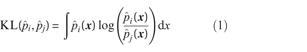
which is a measure of information divergence
33
and relative entropy; it is a metric that calculates the distance between distributions of random variables and indicates the amount of extra information needed to model
Other measures based on density estimates that are explored here are the Hellinger distance, the total variational distance, the Kolmogorov distance and the Area metric. Table 1 provides further details about these metrics and provides their equations. The measures based on density estimates considered in this paper fall into two categories:
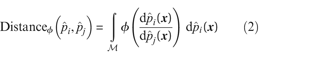
and IPMs with the difference between probabilities,
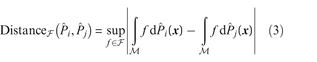
where
The distance metrics based on density estimation that are explored in this paper.
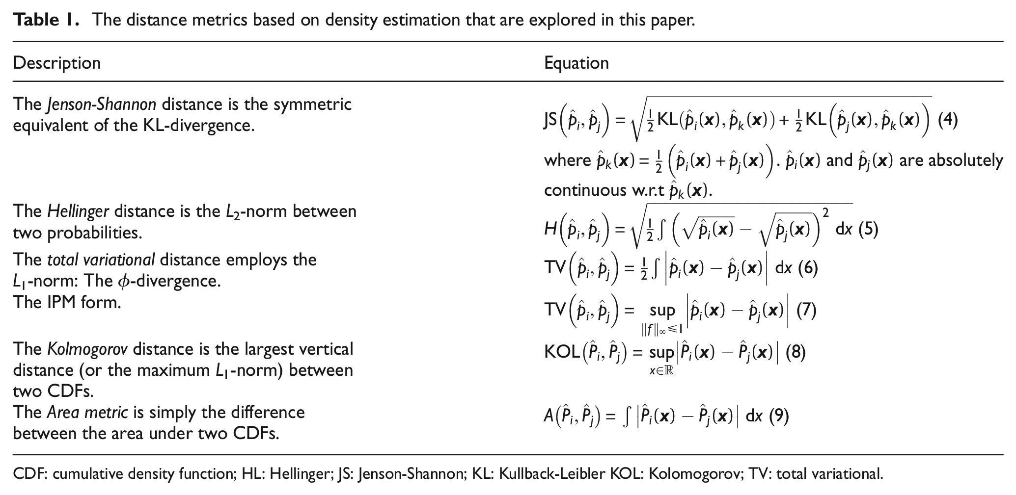
CDF: cumulative density function; HL: Hellinger; JS: Jenson-Shannon; KL: Kullback-Leibler KOL: Kolomogorov; TV: total variational.
Another (true) metric that is considered here is the maximum mean discrepancy (MMD), which circumvents the need for density estimation (this is considered beneficial as there is no universally accepted methodology for conducting density estimations, and they can introduce unwanted variability into the metric formulations). The MMD uses a kernel function to obtain the maximum distance between the mean embeddings of two features or vectors that have been mapped into a reproducing kernel Hilbert space (RKHS). For a more comprehensive understanding, the reader is referred to.34,35 In the past, the MMD has been used in a variety of disciplines, because of its strength in assessing similarity of a range of data types; from time series,36,37 graphical data, 38 images, 39 to attribute matching.34,40 The MMD has been applied successfully in the field of verification and validation in SHM, 32 for domain adaptation,20,41,42 in computer sciences to distinguish between malicious and honest users, 43 and to evaluate the effectiveness of treatment and diagnosis in cancer research 44 to name a few. The biased estimate of the MMD is given by,
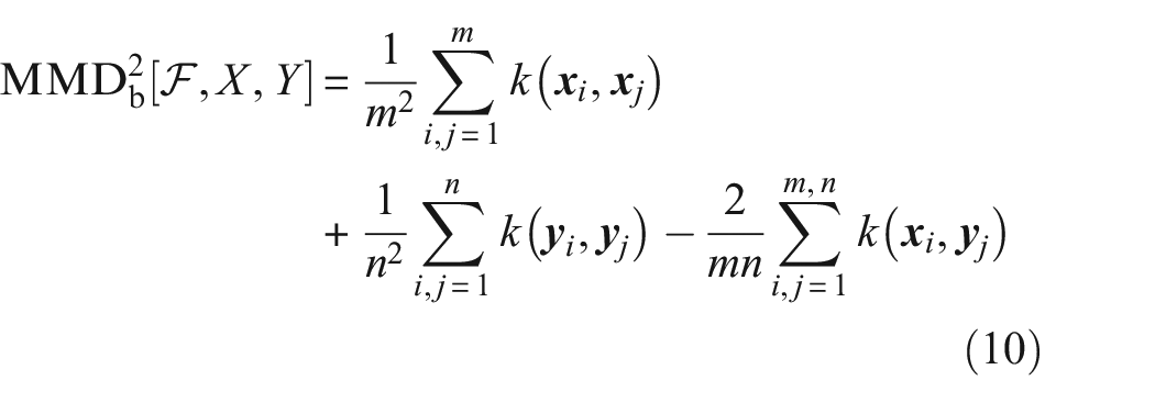
where
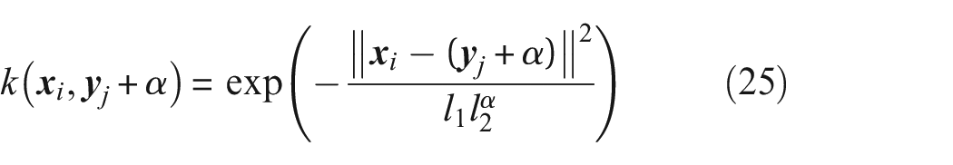
The Gaussian kernel
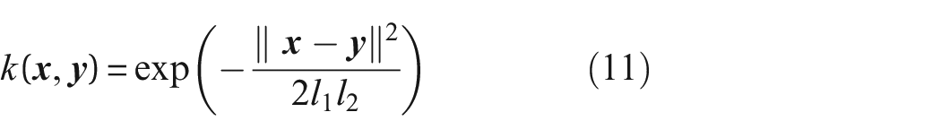
used here, is universal and continuous in the RKHS.
34
The widths of the kernels
Kernel density estimation
Unlike the MMD, the IPM and
To put it simply, the KDE places ‘atoms’ of probability at each observation. The width of these atoms is specified by a window length (or smoothing/bandwidth) parameter and the shape is determined by the choice of kernel type. Usually, the kernels used are symmetric and non-negative. The final density estimate is the sum of these atoms50,51 over a sample set.
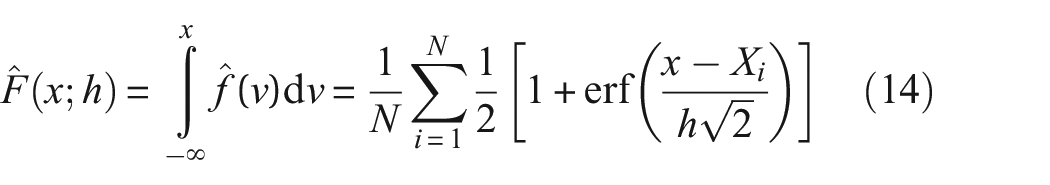
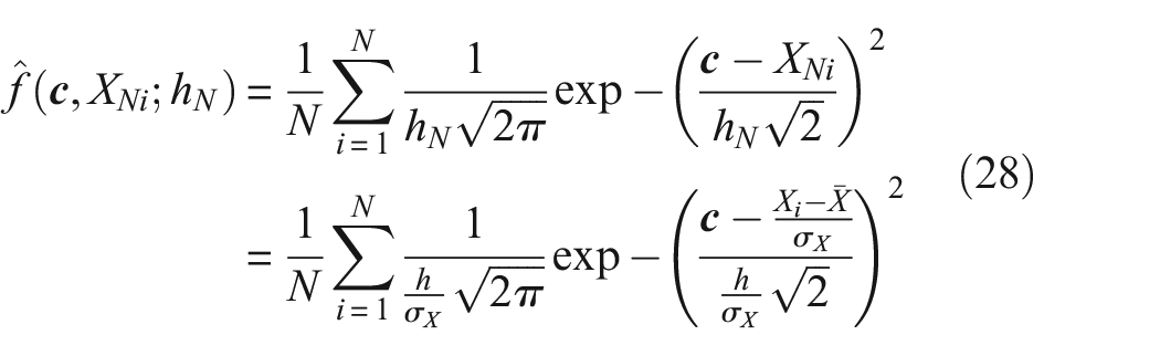
The equation for the PDF with the Gaussian kernel used in this work is,
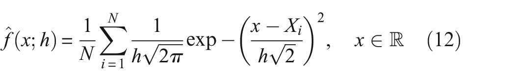
where N is the number of samples,
where n is the number of observations,
where
All methods of density estimation are affected by the chosen parameters, such as the kernel type or the bandwidth of the kernel. As a result, care must be taken when choosing these values, especially in a PBSHM context. For example, when evaluating a metric based on integration of density functions, the integral requires a mesh – or a method of discretising the function – that fixes the x points at which the density functions are evaluated. These points therefore must sufficiently capture the trends seen in the data across the population, in order for the metrics to capture relevant information.
The structure of this paper is as follows. In the next section, a number of typical behaviours observed in SHM data-sets are introduced using a simulated dataset to investigate the response of the aforementioned distance metrics, and assess their suitability in identifying similarity in the PBSHM context. Then, in Section ‘Data normalisation and distance metrics’, using the same simulated dataset, the effects of data standardisation on the behaviour of distance metrics are explored and mathematically formalised; standardisation is an important step in transfer learning and domain adaptation within PBSHM. Furthermore, in Section ‘Case study: similarity of turbines in the Lillgrund wind farm’ the applicability of distance metrics to assess similarity within a population of real structures is investigated via a case study containing data from an offshore wind farm. Finally, concluding remarks are presented and future work is discussed in Section ‘Conclusion’.
Distance metrics response to commonly occurring behaviours in SHM datasets
In order to gain insights and identify behaviours of interest, similarity can be assessed across populations as a first step, using distance metrics. Determining the similarity of data can be useful for, and inform any following steps in the analysis chain. For example, it may be used to extract suitable data for training and testing, for discovering features that are non-representative of the population, for applications such as domain adaptation, 20 to name a few.
In this section, the aim is to determine the suitability of distance metrics suggested in Table 1 to measure similarity of time-domain features in the context of PBHSM. Consequently, the sensitivity of the distance metrics to the transient and permanent changes typically observed in SHM features is studied. By doing so, it may be possible to identify specific metrics that are highly sensitive to a given change in feature behaviour. These differences can stem from EOVs, structural deterioration and even contamination as a result of impediments to the measurement chain (e.g. the sensor network). A simulated dataset that mimics these variations is used in this section. Particularly, the effect of these behaviours on the kernels and density functions that drive the distance metrics are mathematically derived, with a focus on the parameters that underpin these functions. Later, in the case study, examples of these variations acting on a real-world PBSHM dataset are presented.
Typical variations in SHM features
Structures in operation undergo a range of EOVs in their lifetime, for example, temperature changes, wind loading, fluctuating traffic loading (across a bridge, say), etc. Typically, the influence of EOVs on monitoring data (and on any feature therefrom derived), manifests in a change in statistical moments (mean, variance, skewness, etc) in either the time or frequency domain (or both). Commonly in SHM, changes in the mean of the resonance frequencies are tracked for their sensitivity to damage. Naturally, these features are also sensitive to changing temperature and fluctuate accordingly52,53– giving rise to daily and seasonal trends. Other commonly occurring signatures of EOVs are changing variance, 54 here again attributed to temperature, temporary mean shifts8,55 caused by daily changes in wind direction or seasonal changes in temperature, and spikes which can be attributed to, for example, a quick transition to the extremes of the environmental or operational envelope. 56 The presence of structural damage or damage in the measurement chain also affects measurements and features in a similar manner (changing EOVs are often referred to as confounding influences in an SHM assessment for this reason). In this section of the paper, the effect of these commonly observed signatures on a series of candidate metrics is studied. The intention is to assess metric sensitivity and determine how best one might approach an initial analysis that is looking to identify similarities and differences in a population, whether they be from EOVs, damage or other.
To mimic these behaviours of change in frequency, variance and mean, and also to observe their affect on distance metrics within the time domain, a simulated dataset is used where an ‘original’X– data sampled from a normal distribution with a mean of zero and a standard deviation of one, that is,
The presence of typical SHM behaviours are likely to affect the distance metrics. As the metrics are driven by the density functions of the features, the way in which the characteristics of the density functions are affected is explored here. Note that the integrals in Table 1 may be approximated by numerical summations as long as the integration mesh is invariant across all features that are being compared.
Change in amplitude/variance
Changes in variance and amplitude are often observed in SHM datasets as a result of EOVs or damage.
Effect on density estimates
To parameterise such changes in amplitude/variance by

The

to account for the change in variance. As seen in Figures 1 and 2, changes in
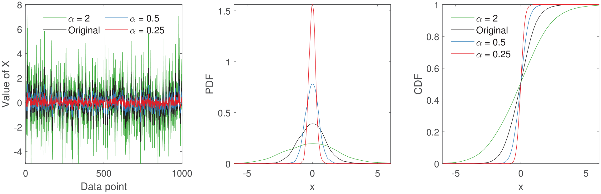
The effect of changing variance of a feature on probability density estimates. Here the amplitude of the original signal is changed to
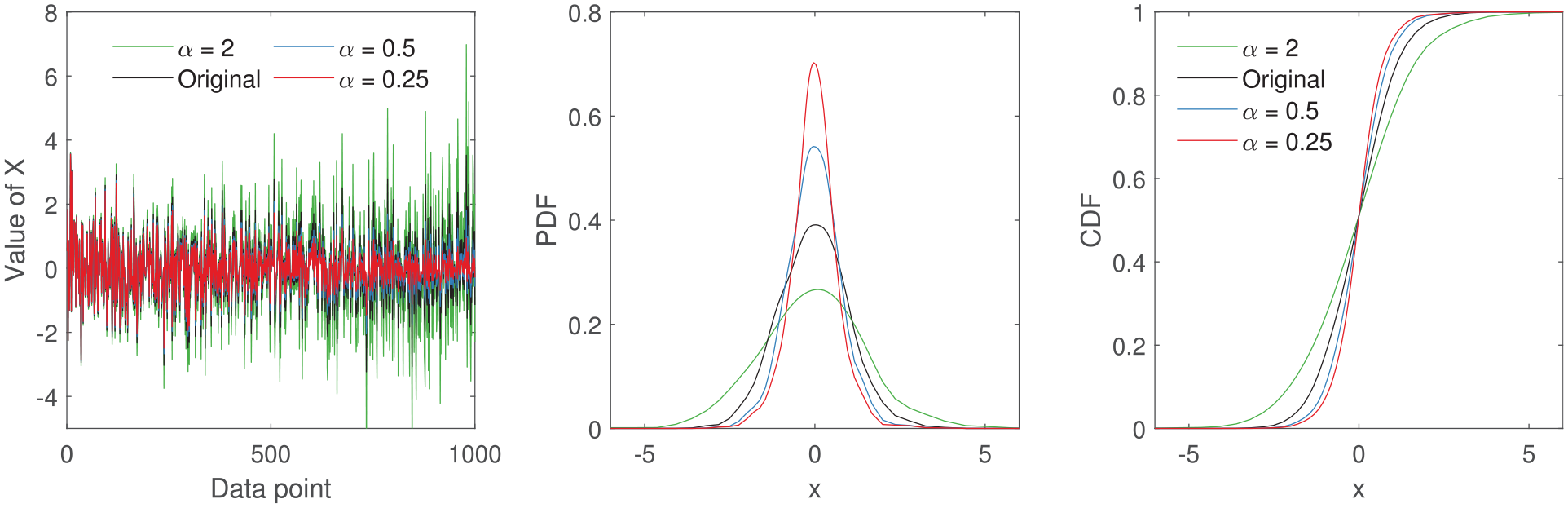
The effect of continuously changing amplitude of a feature on probability density estimates. Here the amplitude of the original signal is incrementally changed from 1 to
If a temporary change in variance occurs (for a small time window where
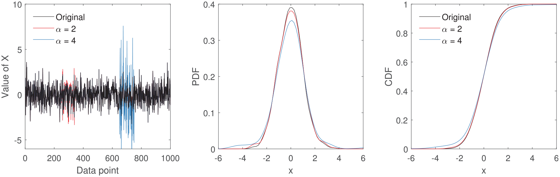
The effect of temporarily changing the amplitude of a feature on probability density estimates. Here the amplitude of the original signal is incrementally changed from 1 to
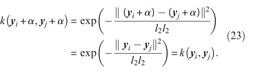
Effect on the Gaussian kernel used in the MMD
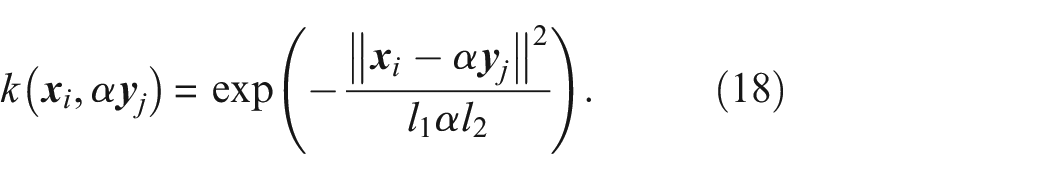
As the Gaussian kernel is employed differently in the MMD compared to KDE, it is useful to understand how the MMD formulation in Equation (10) is affected by a change in amplitude. When calculating the MMD, the Gaussian kernel is not evaluated over fixed intervals. Instead, the kernel gives a measure of similarity between two feature vectors,
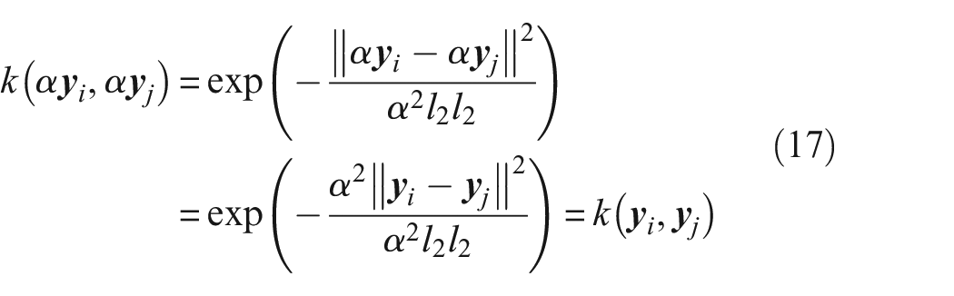
because of the distributive property. It should be noted that the length scale should account for the new change in amplitude. When using the median heuristic to obtain the length scales from
The
If the change in amplitude varies across the feature, the distributive property no longer applies. If
where
affecting the MMD.
Change in mean
The mean of features can alter as a result of EOVs and damage; this is an example of signal shift.
Effect on density estimates
The density functions (in Equations (12) and (14)) translate in mean as,

Here,

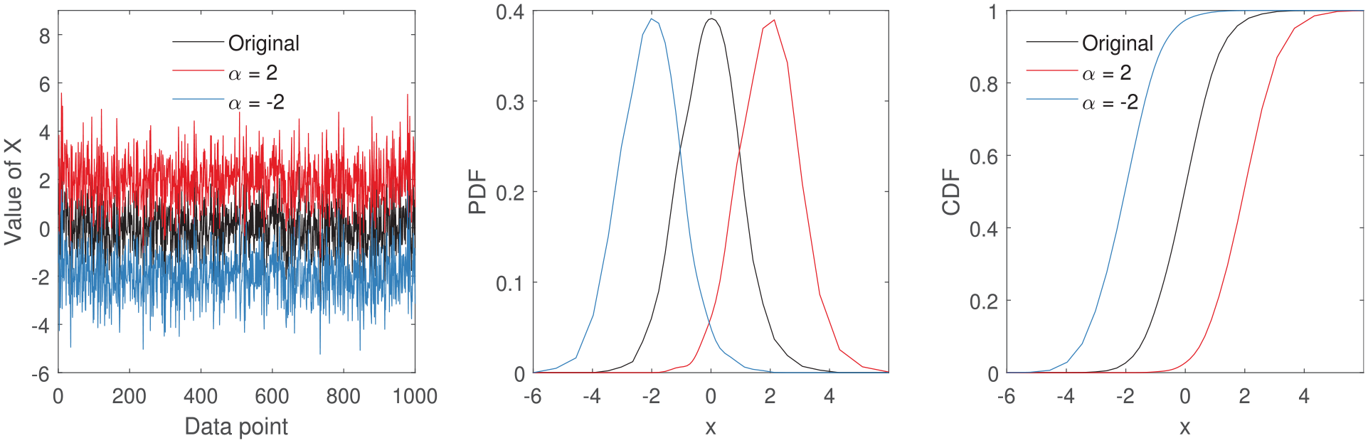
The effect of global mean shift on a feature by a factor

The effect of incremental mean shift on a feature from 0 to
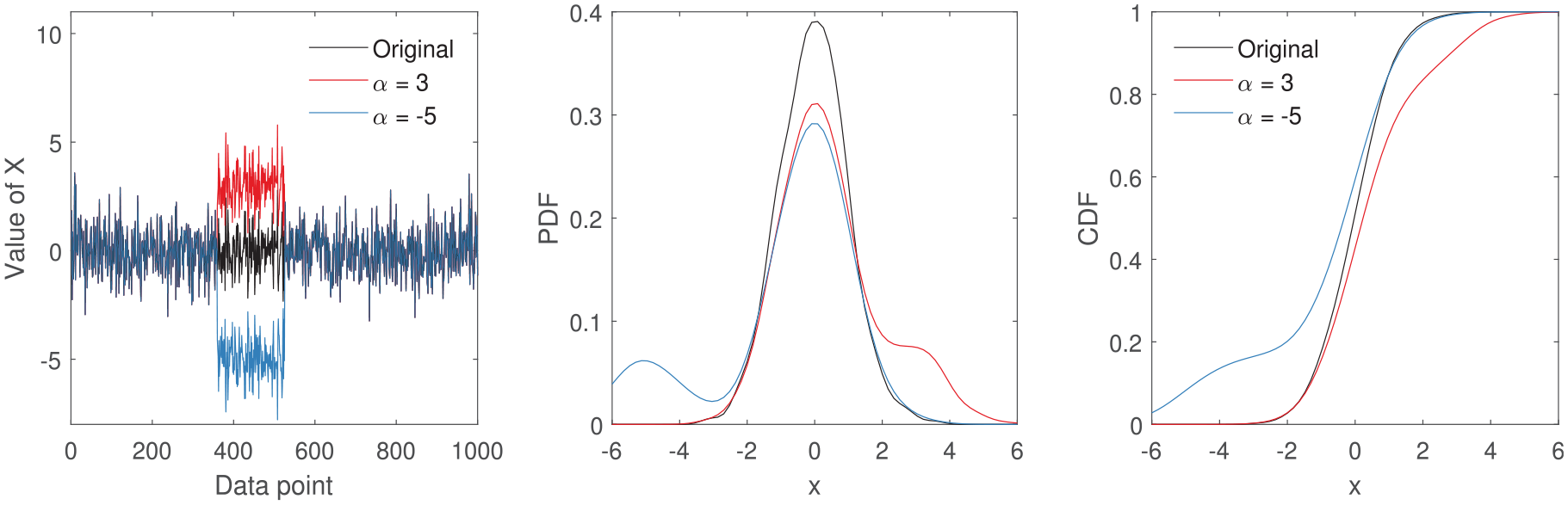
Temporary changes in mean to a feature by
When the entire feature is shifted in mean by a single value of
Incremental changes in the mean shift the density functions and changes their shape, as the variance is also affected (Figure 5). The change in shape resembles an increase in variance, where peak heights are reduced and the width of the peaks are increased. The combination of change in variance and mean affects the skewness of the density functions.
When a temporary shift in mean is present, that is,
Effect on the Gaussian kernel used in the MMD
For the Gaussian kernel in the MMD formulation in Equation (11), if feature X is unaffected and the entire feature Y is translated by a single
However,
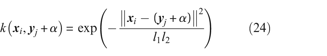
causing the MMD to change accordingly.
If, however, the mean is altered incrementally or if only a portion of the feature’s mean is altered, the variance will be affected and therefore the length scales will also change. Consequently,
showing that changes in mean of one distribution will be detected by the MMD.
Change in frequency
The frequency content of sensor signals can vary during normal operating conditions as a result of EOVs and damage. However, the change in frequency of a feature,

(where
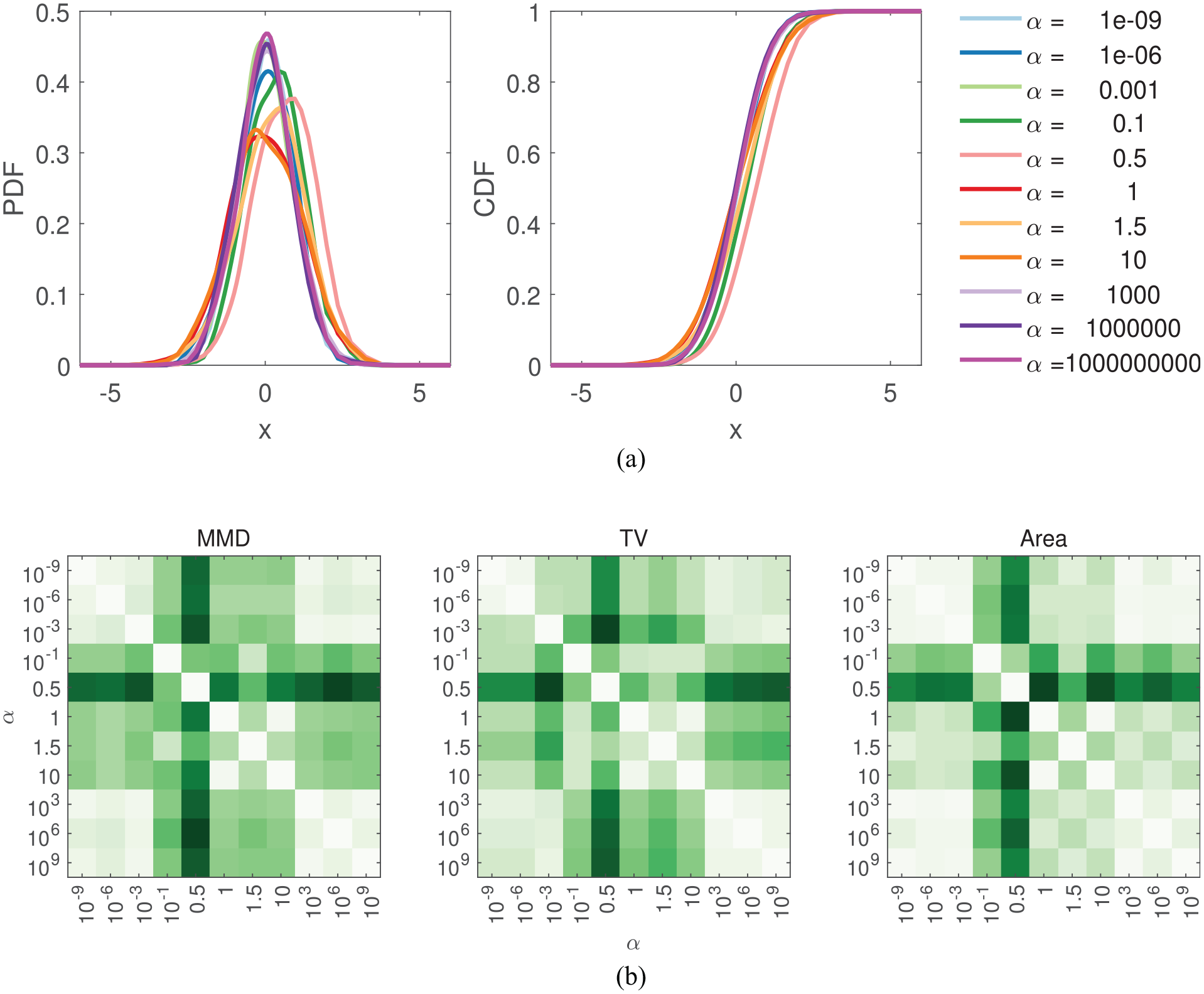
Change in frequency across a wide range and the resulting effect on density functions and distance metrics. One metric based on the PDF, CDF and the MMD are presented here. In (b) the lighter shades represent high similarity and the darker shades represent high dissimilarity. (a) The effect on density functions as the frequency of X is altered by
When the change in
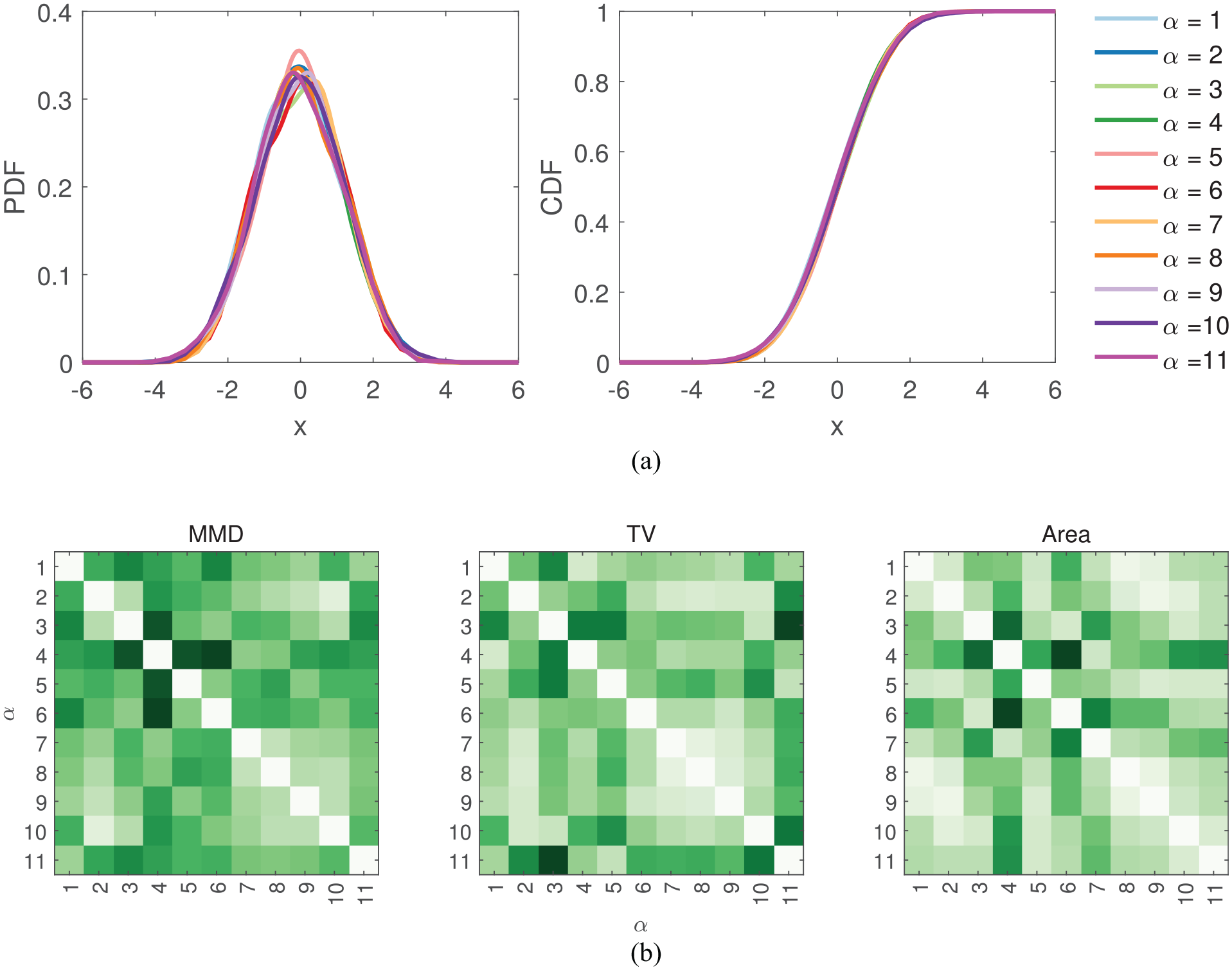
Change in frequency across a relatively small range and the resulting effect on density functions and distance metrics. One metric based on the PDF, CDF and the MMD are presented here. In (b) the lighter shades represent high similarity and the darker shades represent high dissimilarity. (a) The effect on density functions as the frequency of X is altered by
It is clear that the method of employing distance metrics to identify feature changes at the top of the analysis chain suggested here, is unable to effectively capture changes in frequency in time-domain features. Consequently, change in frequency will not be explored further in this paper. However, SHM methods often track frequencies (such as natural frequencies of structures 56 ), across time, where changes in frequencies can present themselves as changes in mean and/or variance. An example of such behaviour is presented in Figure 9, where freezing temperatures alter the natural frequencies of the Z24 bridge 56 – a widely explored case study in SHM. The distance metrics method suggested in this paper will be useful at identifying these changes in frequencies, as they will alter the density functions as seen in Figure 6.
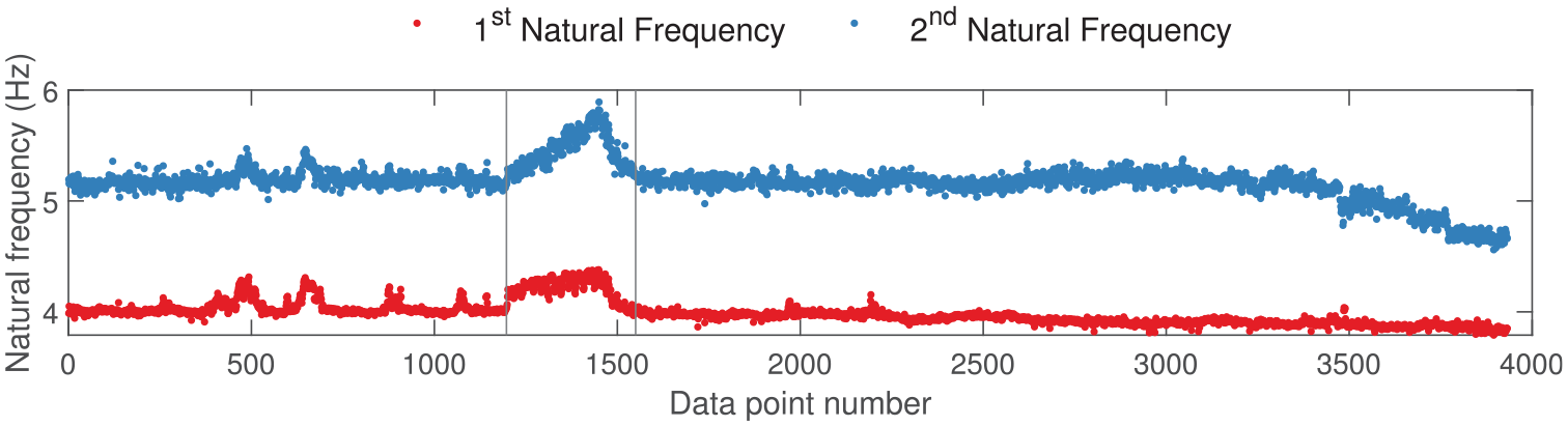
The natural frequencies of the Z24 bridge where changes in frequencies resulting from freezing conditions are highlighted between the two vertical black lines. 56
The response of the metrics to changes in amplitude and mean
For automated similarity/dissimilarity assessment within PBSHM, the method put forward in this paper is to use distance metrics to measure the difference between features collected from datasets. It is, therefore, important that the distance metrics suggested here are reponsive to typical behaviours observed in SHM features. The hope here is that the candidate metrics are able to detect changes in mean and variance of the features and provide insights into the underlying behaviour of the data at the very top of the analysis chain.
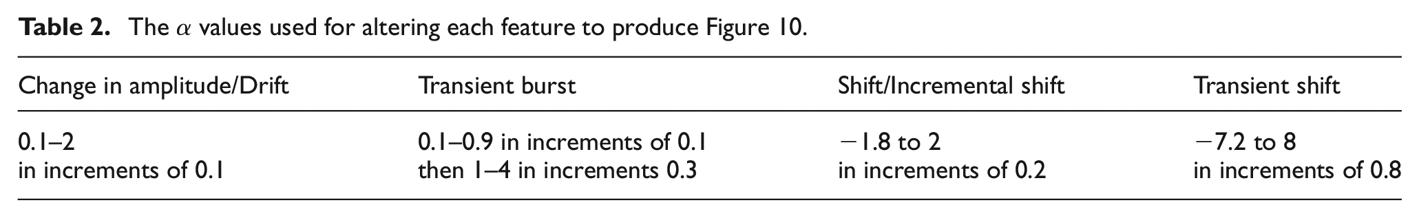
Figure 10 presents how the distance metrics respond when the amplitude/variance of features are altered by
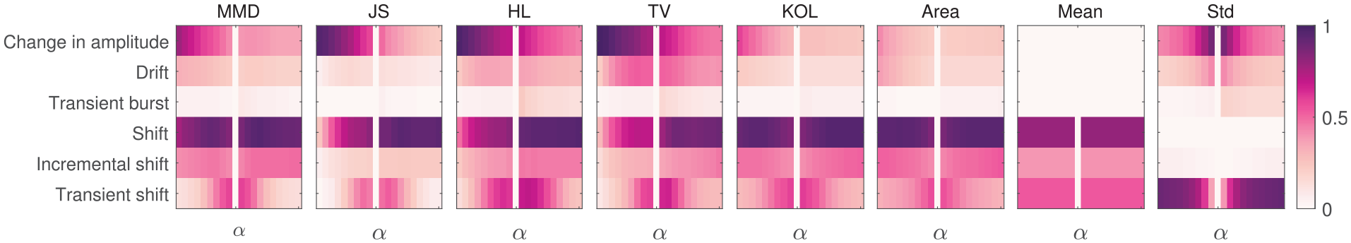
The sensitivity/response of each metric to varying
The
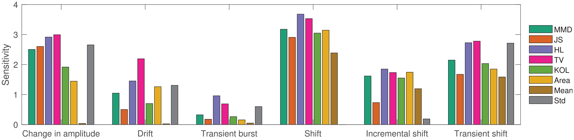
The maximum metric values from each SHM feature presented here to provide an overview of the metric response in Figure 10. The response of the first two statistical moments are also presented here for comparison purposes.
Key insights from Figures 10 and 11 are:
When considering all feature changes (‘Change in amplitude’, ‘Drift’, ‘Transient burst’, ‘Shift’, ‘Incremental shift’, ‘Transient shift’) in Figure 10, the distance metrics show a higher sensitivity overall than simply using ‘Mean’ and ‘Std’; for some features, the maximum values of ‘Mean’ and ‘Std’ are very small/negligible in Figure 11.
The first statistical moment ‘Mean’ is unsuitable for detecting features based on an amplitude/variance change as those features do not drive a change in mean. Conversely, the ‘Std’ has a limited or null response when identifying global and incremental shifts in mean, as the change in standard deviations of the features are negligible. It is, however, able to detect transient shifts in mean as the standard deviation increases as a result of the multiple modes (as seen in Figure 6).
Across the range of
Variance changes for a short window (‘Transient bursts’) evoke the smallest response across all distance metrics. HL and TV metrics show the highest sensitivity where they are less sensitive to small variations compared to large variations. As short ‘bursts’ of variance increase can indicate the presence of damage or a change in conditions, the HL and TV metrics are preferred here.
When considering a global change in amplitude, all distance metrics based on the PDF, the MMD and ‘Std’ present a large response. The peak height and area of the PDFs change readily with varying amplitude, as seen in Figure 1. The distance metrics are more sensitive to reduction in variance (or when
The metrics are more sensitive to small transient shifts compared to large ones. The statistical moments are also relatively sensitive to transient shifts.
The aforementioned changes in variance and mean clearly affect the density functions and their statistical moments, and in turn drives the changes in distance metrics. HL and TV metrics present the highest overall response across all features and are well suited for assessing similarity within SHM datasets. It should be noted that the MMD performs similarly to HL and TV (often presenting the third highest sensitivity within the distance metrics), and should be given serious consideration here as the most suitable candidate, because it negates the need for density estimation. This is a promising result, as it is preferable to avoid density estimation where possible.
Table 3 presents the order in which each metric prioritises a feature according to sensitivity. The MMD, JS and HL metrics show similar priorities here, whereas the TV, KOL and Area metrics have different preferences. The Area metric is unique in that it is more sensitive to changes in mean than variance. Although the difference between the sensitivity responses are relatively small across all metrics – with no obvious front-runners for any given feature (Figure 11) – the priorities of the metrics suggest that some are more sensitive to specific features over others. Therefore, the MMD, JS, and HL metrics are expected to behave similarly when identifying features, whereas, TV, KOL, and Area metrics are expected to highlight different types of features. On this account, commonly occurring behaviours within new datasets may be identified by using a combination of distance metrics, allowing for fast and automatic information retrieval and similarity assessment.
The sensitivity of each metric to each feature ordered from the most sensitive to least sensitive. This table gives an indication of which type of SHM feature each metric prioritises during automated similarity assessment.
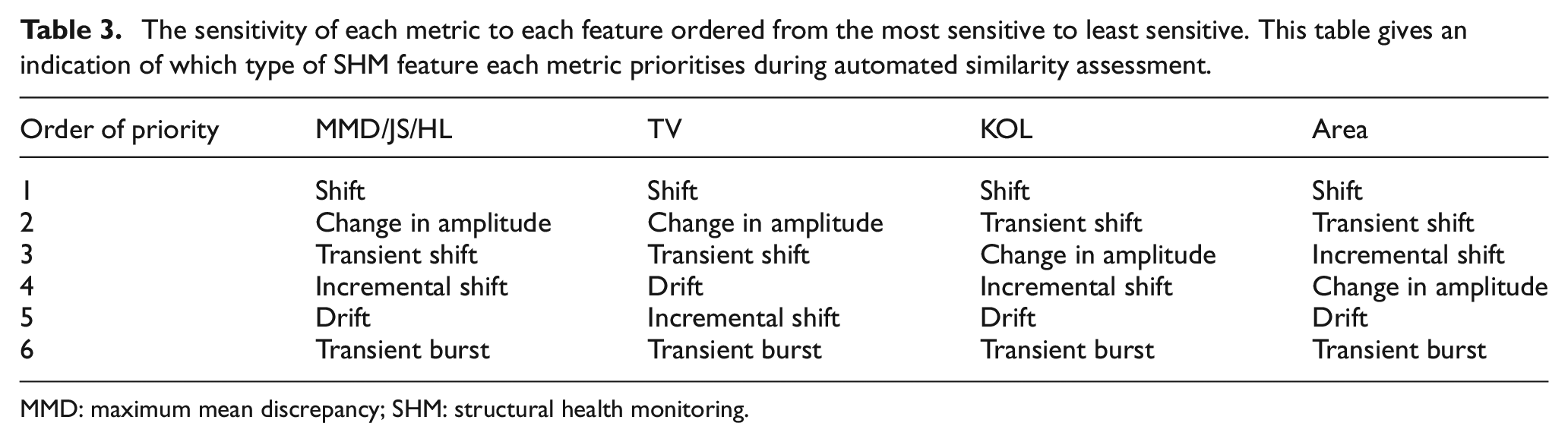
MMD: maximum mean discrepancy; SHM: structural health monitoring.
By using a simulated dataset, in this section, the responses of candidate distance metrics to commonly occurring SHM features are explored. It is clear that the metrics are well suited for identifying features (especially over simple analysis using the first two statistical moments), where some metrics show a preference for identifying certain features over others. As a result, a given metric can give an indication of the type of features present in a signal without manual inspection. The results presented here using the simulated dataset are satisfactory pointers towards generalisation, because in a population-based setting – particularly within a homogeneous population where the behaviour of the data within a given window is assumed to be the same/very similar (Even in heterogenous population examples, feature similarity is important to avoid negative transfer23,26) – the metrics will not identify differences between general trends as
A note on real-time analysis of population data using distance metrics. Although not implemented in this paper, it is noted here that for PBSHM, it is possible to use these metrics to track the behaviour of structures over time, using a moving window. Care must be taken when discretising the density functions in this case, because an inadequate range could diminish the effect of unexpected SHM behaviours or highlight normal behaviours as abnormal. As the MMD formulation does not require the calculation of density functions, it is perhaps better suited for real-time analysis. In this case, a suitable moving window length can be chosen a priori that captures the general fleet-wide trends in historical data, offline. The data that are used to set the window length should be collected during normal operating condition in order to ensure that abnormalities (deviations from the normal condition) can be detected during real-time implementation.
The computational complexity of calculating the MMD is
In the next section, the effect of normalisation of the data on the metrics is discussed; normalising or standardising the data to have zero mean and unit standard deviation is a common pre-processing step in SHM analyses. Normalising removes the effects of mean and variance on the density estimations. As a result, it is possible to determine if a given metric is sensitive to higher-order moments that may be present as a result of variations within the data. In PBSHM applications that utilise transfer learning, normalisation can be vital for aligning domains for domain adaptation. 22 Techniques such as normal condition alignment can help move data and change the size of the space they occupy, in order to facilitate better decision boundaries that separate the data well, and allow easy comparison between domains. Foregoing alignment can sometimes even lead to negative transfer. The next section of this paper explores how normalisation can affect data and therefore the ability to find similarities using distance metrics, if the calculation of the distance metrics should be altered to aid normalisation, and how to analyse the results from normalised data.
Data normalisation and distance metrics
In conventional SHM, distance metrics can be used to identify whether structures are operating under normal (undamaged) conditions, or if damage has occurred, where a large distance between the normal and damage conditions is preferred. In PBSHM, it is desirable to reduce the distance between the data from normal conditions of different structures in a population to aid positive transfer in instances such as when attempting domain adaptation.20,22 Here, distance metrics are used to identify the target label-set that is the closest match to the source domain. Normalising the source and target domains by their respective normal operating condition helps align the data by the normal condition. This form of normalisation is beneficial to transfer leaning, as learners are notoriously ineffective when translation has occurred between source and target data.59,60 Normalisation can, however, mask the effects of temporal and spatial EOVs; the dynamic response of the structures can be altered by wind, thermal and induced vibrations, change of material properties and boundary conditions.8,61
In this paper, distance metrics are used to find similarity and information within a population when there is no knowledge of the underlying data structure. The assumption is that little to no information is available on the condition of the structure (from which the data were collected), or the data itself. In the previous section, distance metrics were tested against a number of typical behaviours in SHM features in order to determine their suitability at detecting changes and assessing similarity. These behaviours usually have an affect on the characteristics of feature distributions. In this section, normalisation is employed to eliminate the effects of lower-order moments from the data and highlight features containing higher-order moments such as skewness and kurtosis. Given that higher-order moments can indicate the presence of transient shifts/drifts in the data, normalising in this context may be helpful in identifying features that are affected by unexpected behaviours. Consequently, a single distance metric value used on absolute and normalised data may indicate useful information about the underlying structure of the data.
Normalisation in the form of standardisation is an alignment step that can be applied to data.62–64 Standardisation translates and scales the data collected from structures by subtracting the mean and dividing by the standard deviation. When applied on a structure-by-structure basis – also referred to as self-standardisation – the resulting data from each structure has a mean of zero and a unit variance. Often it is used to move data to a similar space where comparisons between the data are meaningful. Standardisation can also reduce the condition numbers of matrices, allowing for numerical accuracy when computing their inverse. It is important to note that metrics cannot be used on self-standardised data to find differences between datasets because global transformations have not been conducted on the data; the mean and variance of each dataset are likely to be slightly different and, therefore, each dataset will be altered differently during self-standardisation. In this section, self-standardising is used to investigate the origin of the differences seen in PBSHM datasets.
Figure 12 visually presents the effect of self-standardisation on the density functions that drive the distance metrics. Here, the commonly occurring features in Figures 1 to 6 are used for demonstration.
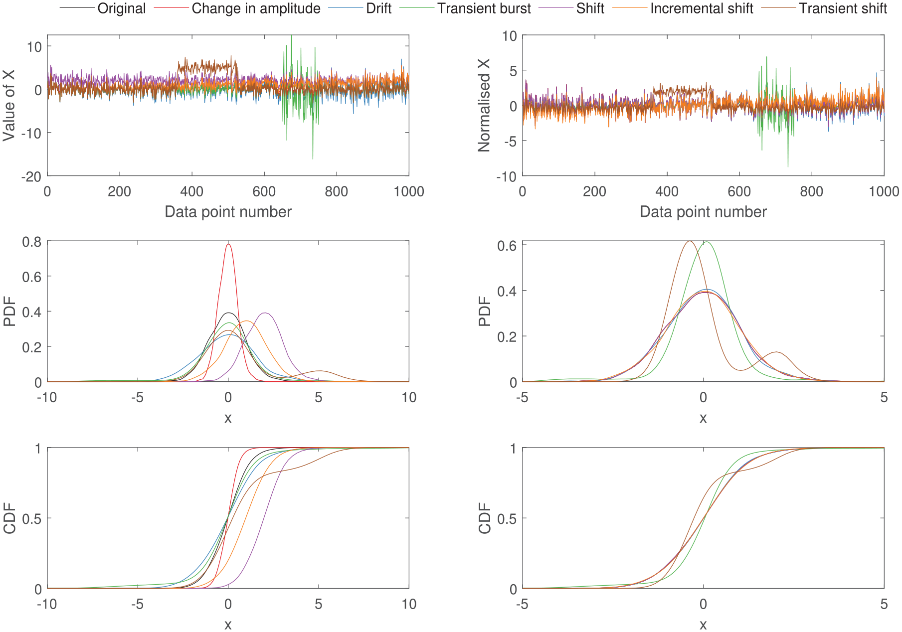
The effect of standardising on density functions is presented using the commonly occurring SHM behaviours. Standardising (figures on the left), leads to effects from changes in amplitude/variance and translation to reduce, and highlights transient changes.
Data standardisation and the IPM and
-divergences
The IPM and
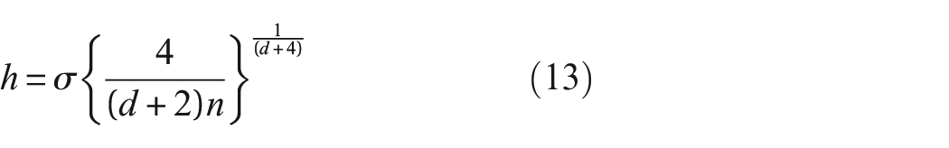
When the data are self-standardised, the bandwidth parameter, h (in Equation (13)) becomes,
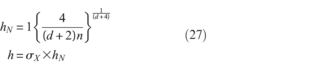
because the standard deviation of the self-standardised data
where
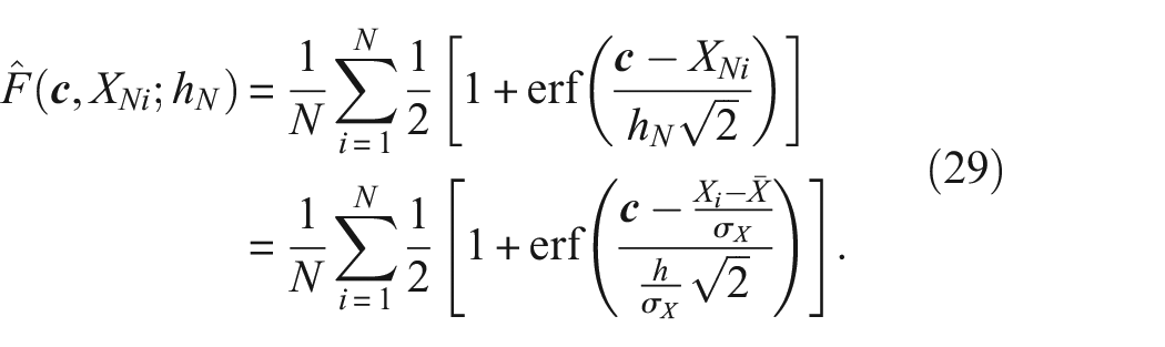
Therefore, in a PBSHM setting, the discretisation and the smoothness of the density functions are affected when the data are self-standardised. As a result, these values should be re-evaluated when obtaining density functions for self-standardised data. Equations (28) and (29) can be fed back into the metric formulations where the integrals can be treated as sums, because the discretisations
Data standardisation and the MMD
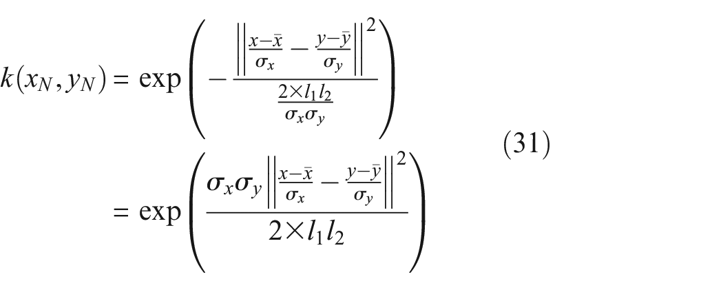
As the random variables x and y from Equation (10) are moved to a similar space by standardisation, the value of the MMD is expected to change because it is a measure of difference between the mean embedding of two distributions. As the Gaussian kernel for the MMD is calculated on the data from two distributions (Equation (11)), the length scales can be separated.
When both variables are from the same distribution, the normalised kernel is equal to the non-normalised kernel, that is,
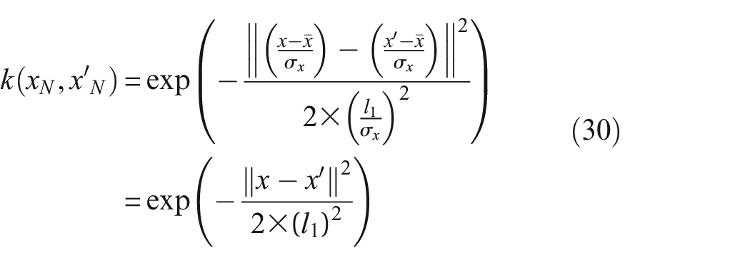
where
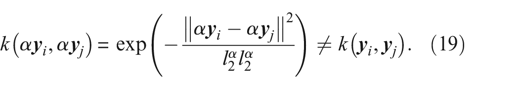
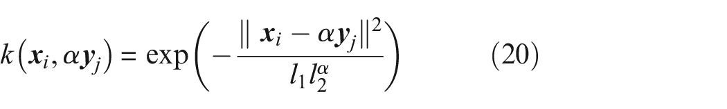
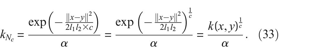
It is also interesting to note the effect of altering the length scales of the kernel when standardising, because obtaining the optimum choice of kernel size is an current research topic, and therefore the length scales are subject to change.
34
For example, if the relationship between
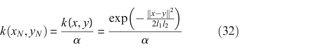
becomes,
Again, as the MMD is a true metric that circumvents the need for density estimation, it may be preferred over metrics based on density estimates when used for preliminary analysis; this is because, the discretisation step required for density estimates (on both absolute and self-standardised data), can be avoided when using the MMD.
The response of distance metrics to self-standardised data
In this section, the focus is on exploring the effect of self-standardised data on the response of distance metrics. This is an important consideration for PBSHM because, standardisation is a key alignment technique used to bring domains into a similar space for transfer learning. Furthermore, standardisation can be used to reduce the effects of the first two statistical moments on the data, thereby increasing the metric’s sensitivity to higher-order moments. It is hoped that standardisation will help to identify interesting features in the data that were previously masked by the mean and variance. Earlier, in Figure 12 it was found that transient behaviours are highlighted after standardisation as they tend to contain higher-order moments. The aim here is to find metrics that are sensitive to those characteristics. Again, the commonly occurring behaviours introduced in Section ‘Distance metrics response to commonly occurring behaviours in SHM datasets’ are used here for demonstration.
When considering the commonly occurring SHM behaviours, Figure 13 show how each distance metric responds to self-standardised data. As with Figure 10, the response of ‘Mean’ and ‘Std’ are presented here for comparison between the distance metrics and the first two statistical moments. The results in 13 are combined with the absolute case in Figure 10 and normalised between [0,1] for ease of comparison. The corresponding self-standardised metric values for constant changes in amplitude, and constant mean shifts are not presented here because self-standardising these altered features leads to metric values of zero. In these figures,
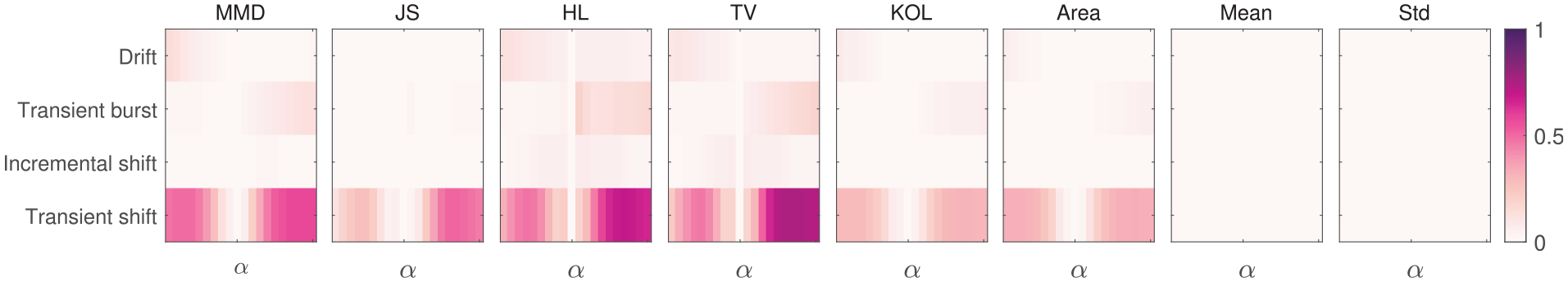
The sensitivity of each metric to varying
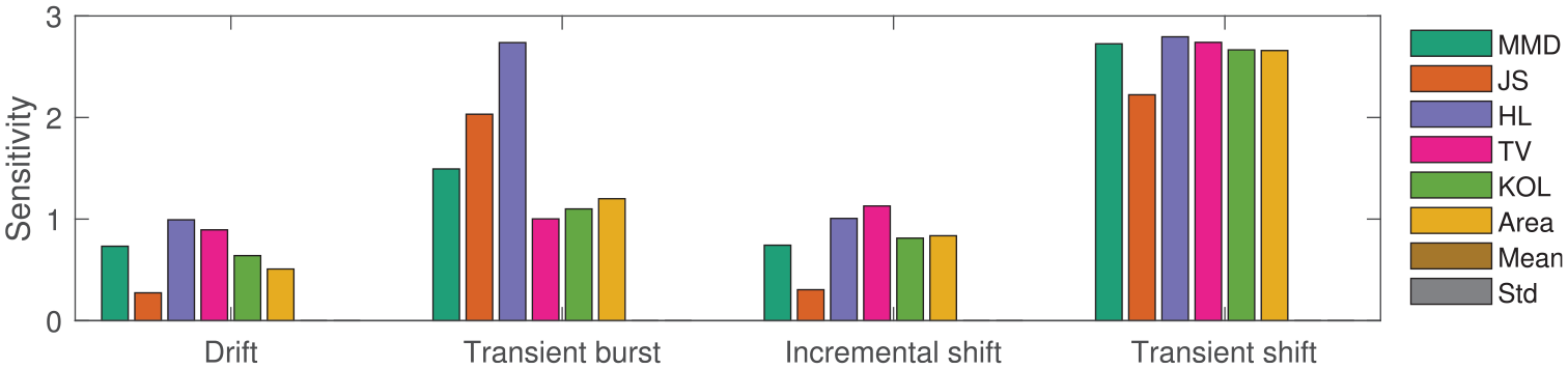
The maximum metric values from each SHM feature presented here to provide an overview of the metric response in Figure 13. The response of the first two statistical moments are also presented here for comparison purposes.
The key observations from Figures 13 and 14 and comparisons between the absolute case in Figures 10 and 11 are:
Unsurprisingly, the metric responses are markedly reduced when assessing self-standardised data because the effects of mean and standard deviation are removed.
The first two statistical moments ‘Mean’ and ‘Std’ are unable to detect any changes in the features within self-standardised data, making them unsuitable for similarity assessment in PBSHM where the data are standardised.
Unlike the first two statistical moments, the distance metrics show some response to the feature changes, with a relative high response towards transient shifts.
The distance metrics based on the PDF and the MMD present a higher sensitivity to transient bursts in the self-standardised case in Figure 14 compared to the absolute case in Figure 11 because, the higher-order moments such as skewness and kurtosis are highlighted as the data are standardised (as observed in Figure 12).
As data are standardised, metrics are more responsive to transient behaviours over incremental behaviours.
These results show that there are advantages to undertaking data standardisation in the context of identifying commonly occurring SHM features using distance metrics. Transient effects are especially highlighted in the standardised case, when the effects of general trends (overall mean and variance changes) are diminished. As transient features can be indicative of damage and EOVs, it is useful to undertake data standardisation to identify them.
Table 4 presents the order of priority for each metric as the data are standardised, that is, the standardised features that each metric is sensitive to, ordered from most to least. The results here show that there is a high level of uniformity across the candidate metrics, except for the TV metric. The TV metric is more sensitive to incremental shifts over transient bursts; perhaps because incremental shifts not only shift the data but also reduces the area under the PDF, the TV metric (in the
The sensitivity of each metric to each standardised feature ordered from the most sensitive to least sensitive. This table gives an indication of which type of SHM feature each metric prioritises during automated similarity assessment of standardised data.
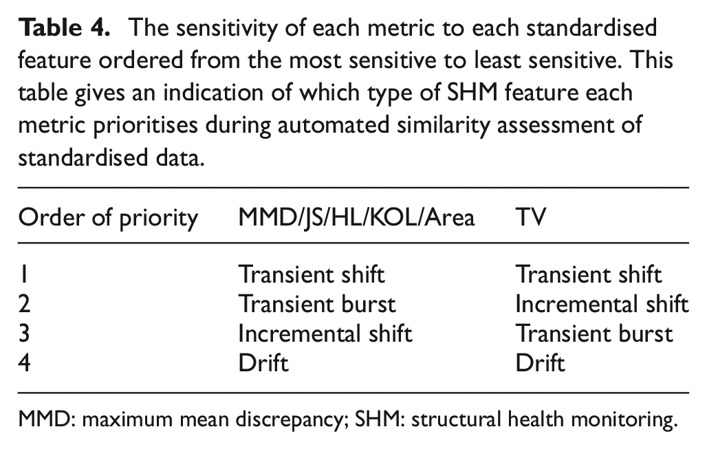
MMD: maximum mean discrepancy; SHM: structural health monitoring.
The recommendation here is therefore to assume that the metrics based on the PDF are likely to identify overall trends when using absolute data, and highlight transient behaviours when the data are standardised. When considering metrics based on the CDF, transient shifts can be identified from absolute data. As a result, when using absolute data, a combination of HL/TV and KOL/Area should detect a variety of SHM features from the dataset automatically. In the standardised case, the TV metric can be used alongside HL to identify a range of transient and incremental features.
Overall response of the distance metrics
Figure 15 presents the overall performance of the metrics when considering the SHM features in both absolute and standardised cases (six absolute and four standardised features). The x-axis of the figure represents the ‘score’ of each metric; the score is calculated by identifying the maximum response of each metric to each feature and giving a value of one for the most sensitive metric and a value of eight for the least sensitive metric (as there are eight metrics assessed in total: six distance metrics, two statistical moments). A metric can have a total score between values of 10 and 80 where a value closer to 10 suggests that the metric has a high sensitivity to all SHM feature and a score of 80 suggests that the metric is insensitive to all SHM features. The scores are plotted against the variance of the score in the y-axis. A small variance suggests that the response of the metric was similar across all features, whereas a high variance of score suggests the response of the metric varied significantly from feature to feature. The best overall metric should, therefore, have a low score and a low variance. In Figure 15 two dashed lines separate the metrics at 50% of the score (vertical) and 50% of the variance (horizontal). Those in the bottom left corner are the best performing metrics from the chosen candidates. Within this quarter, the HL has the lowest score and the MMD has the lowest variance. Again, as the metrics based on density estimation require a discretisation mesh to be selected, the similar performance of the MMD is advantageous for feature assessment at the start of the analysis chain.
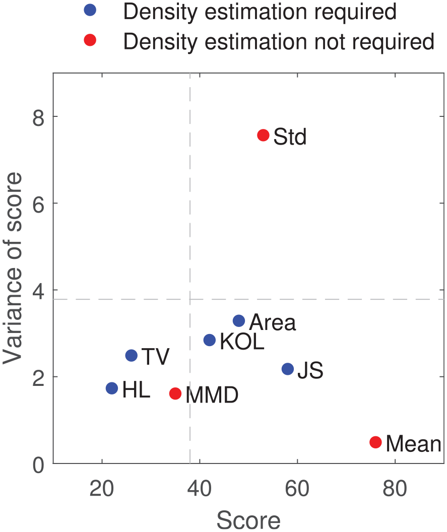
The overall performance of the metrics across all absolute and standardised features. The metric with the largest response has the lowest score. The metric with the lowest variance performs similarly across all features. The best overall metric should present a low variance and a low score. The dotted dashed lines indicate 50% of the score and variance.
The results from the simulated dataset suggests that the distance metrics chosen in this paper are suitable candidates for detecting typical SHM behaviours. It is clear that using a combination of metrics across absolute and standardised data can give insights into dissimilarity across populations as well as provide an indication of what type of features are present within the data automatically. These findings are incredibly helpful for PBSHM, where manually analysing data to find suitable data for training and testing or transfer learning is an impossibility. In order to validate these findings and to understand whether these metrics are flexible in identifying SHM features from measured data from operational structures, a case study is presented next. The case study focuses on identifying similarity/dissimilarity of features collected during a year-long monitoring campaign of a wind turbine fleet.
Case study: similarity of turbines in the Lillgrund wind farm
This case study investigates the use of distance metrics to automatically identify similar/dissimilar behaviours within SHM features collected from a population of wind turbines. This is a homogeneous population, which is a sensible starting point for population-wide assessment. Modern wind turbines continuously collect data pertaining to environmental and operational conditions. Each turbine collects data from multiple channels, usually at ten-minute intervals. The available data for analysis, therefore, grows with population size. On that account, there is a clear need for fast and automated analysis for PBSHM.
The aim here is to gain an understanding of the effectiveness of the investigated distance metrics, at identifying interesting features from real, operational structures, in order to evaluate whether they can be used for automated data assessment in PBSHM. The metrics will be tested on absolute and standardised data as before, to determine whether normalisation is helpful and to discover transient behaviours. If successful, the hope is that these metrics will be used to group together structures with similar behaviours, and reduce the burden on transfer learners to achieve positive transfer, by establishing that the underlying distributions of the domains are similar. Furthermore, the assumption is that identifying dissimilarities within the turbines should indicate unexpected EOVs or damage.
To reiterate, the assumption in this paper, and indeed in this case study, is that the similarity assessment is undertaken at the very start of the analysis chain where little to no information about the data is known. The aim here is to automatically gain knowledge of the data collected from an entire population, reducing – or even alleviating – the need for time-consuming manual analysis.
The Lillgrund wind farm and the SCADA dataset
Located between the Swedish and Danish borders, the Lillgrund wind farm has 48, 2.3 MW wind turbines. 65 This is a homogeneous population, as all the structures are nominally identical, but with varying boundary conditions.1,3,4,20 Each turbine is fitted with a Supervisor Control and Data Acquisition (SCADA) system that collects and saves data from a range of sensors at ten-minute intervals. Henceforth, the 48 turbines in the Lillgrund wind farm will be denoted T1 to T48.
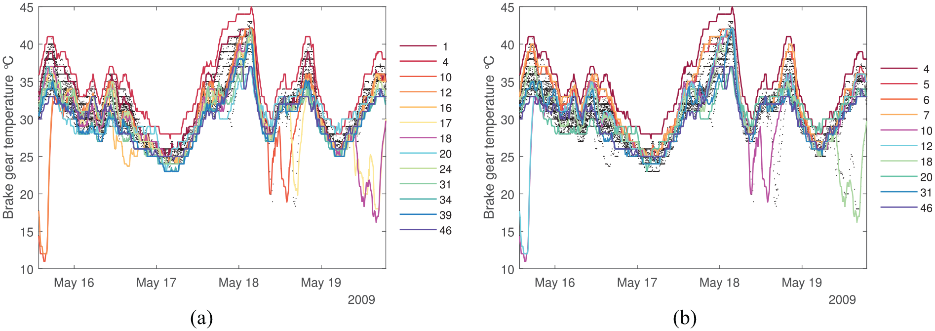
In this work, the brake-gear temperature data collected during the year 2009 are studied (Figure 16). This particular feature is chosen because of its sensitivity to daily temperature variation, and also because it includes behaviours such as shifts in mean, change in variance and transient mean shifts (such as those explored in Sections ‘Distance metrics response to commonly occurring behaviours in SHM datasets’ and ‘Data normalisation and distance metrics’), that may be indicative of operational conditions or damage. To ease the computational burden, a window of data from the middle of May is chosen for analysis. The first step in the analysis process is to identify the most similar and dissimilar turbines within the fleet.
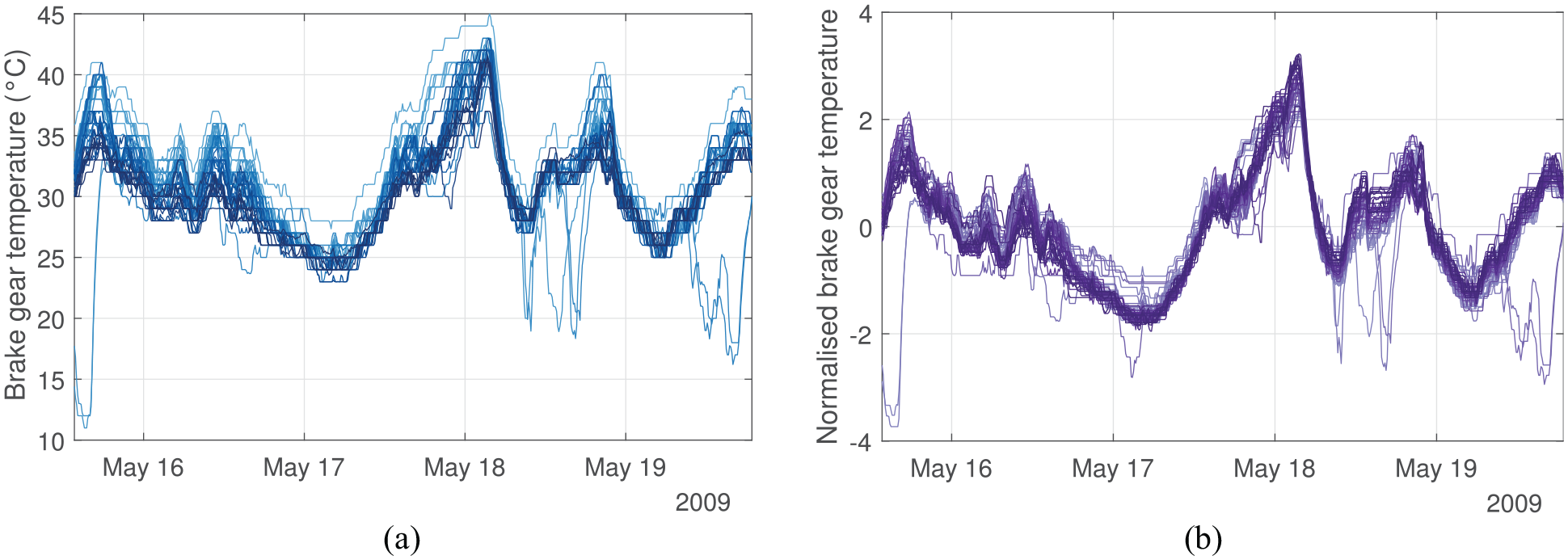
Brake-gear temperature of the 48 turbines in the chosen time window. Some anomalous behaviours can be seen here, where data appear outside of the general trend. Distance metrics may help in identifying these anomalous behaviours. (a) Absolute values and (b) normalised values.
Results and discussions
The results calculated by the distance metrics are presented in Figure 17 in the form of confusion matrices where one-to-one comparisons are made across the population. The darker shades in these figures signify dissimilarity whilst the lighter shades indicate similarity. There are clear differences between the absolute and standardised cases here, suggesting that standardisation has helped identify different turbines to the absolute case, most likely as a result of transient behaviours. The metrics show that a significant number of turbines have high similarities across the population, suggesting that they can be used for transfer learning. This result is a strong indication that the underlying distribution of the general population is similar, which is evident in Figure 16.
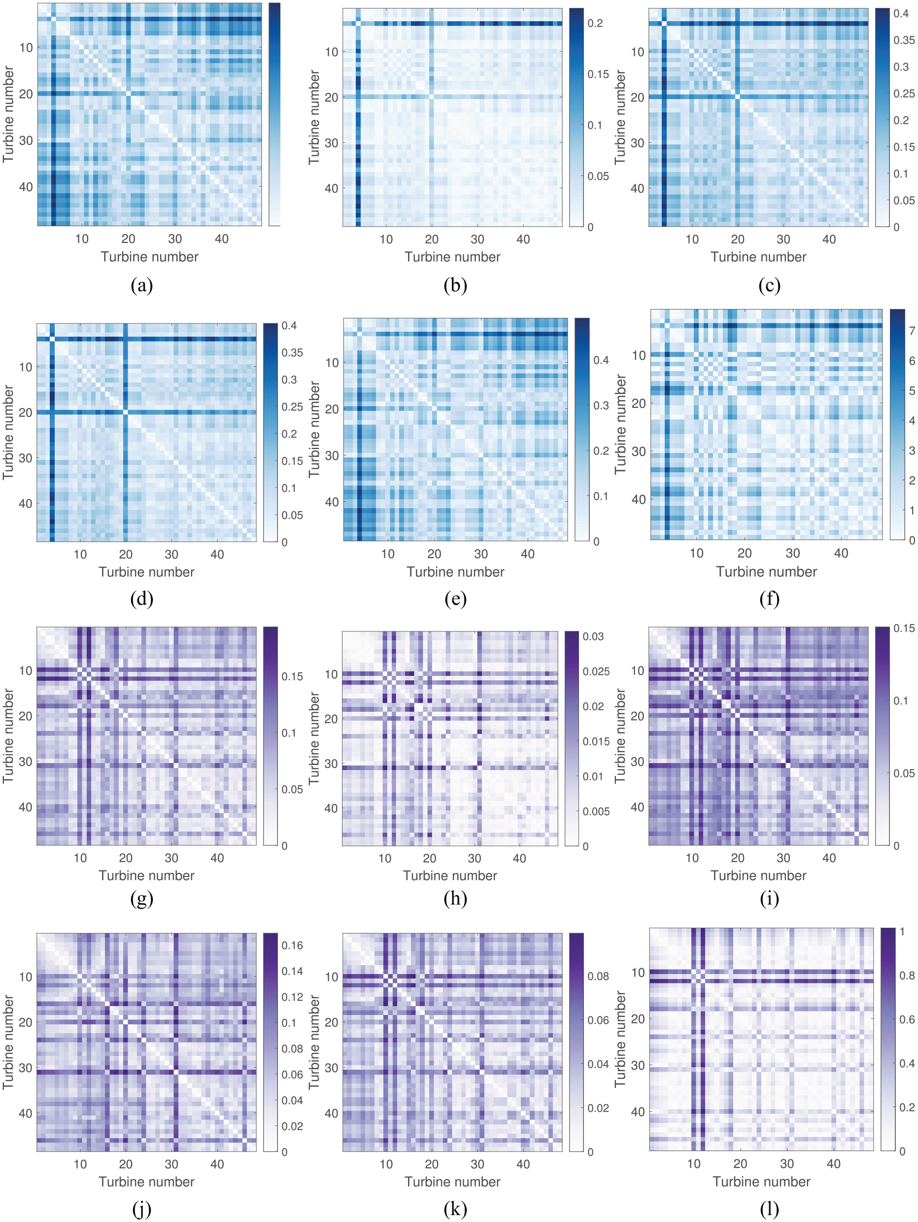
The confusion matrices showing distances calculated by metrics using absolute and standardised data. (a) MMD absolute, (b) JS absolute, (c) HL absolute, (d) TV absolute, (e) KOL absolute, (f) Area absolute, (g) MMD normalised, (h) JS normalised, (i) HL normalised, (j) TV normalised, (k) KOL normalised, (l) Area normalised.
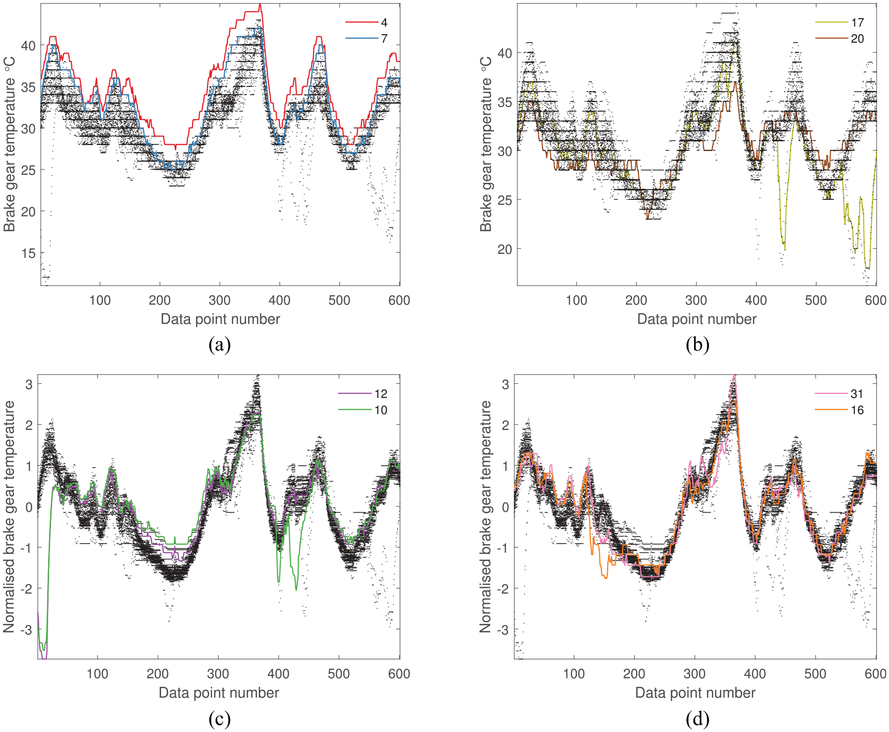
One of the most interesting observations from the confusion matrices is the interaction between two of the most dissimilarly behaving turbines (T10 and T12), in the self-standardised case. It is clear that, even though the distances between data from T10 and T12 are consistently large compared to the rest of the population, the distances between each other are relatively small according to most metrics. This finding suggests that the anomalous data from these particular turbines actually behave similarly to each other and could be an indication that the underlying mechanisms or forces driving these behaviours are also the same. This result illustrates the purpose of PBSHM in a number of ways. For example, if presented with a dataset that contains healthy and damage-state data, it may be possible to identify other datasets that are undergoing the same mechanisms, and detect damage prior to failure using this method for guidance. If the dissimilar behaviour is a result of EOVs, it may be possible to group the relevant structures together and label them appropriately. On the other hand, T10 deviates from T12 around data points 400–450 (highlighted in Figure 18(c)), but that does not reduce the similarity between them, in comparison to the data from the rest of the population, across the window. This result shows that a temporary variation is not as significant for the metrics when the overall trend is very similar, and also demonstrates the importance of the window in which the metrics are calculated; temporary variations may be masked by more persistent trends, resulting in misleading conclusions.
The absolute and normalised brake-gear temperatures. Highlighted here are the most dissimilar turbines identified by the distance metrics. (a) MMD and KOL absolute, (b) JS, HL, TV and Area absolute, (c) MMD, JS, HL and Area normalised, and (d) TV normalised.
Identifying common SHM features
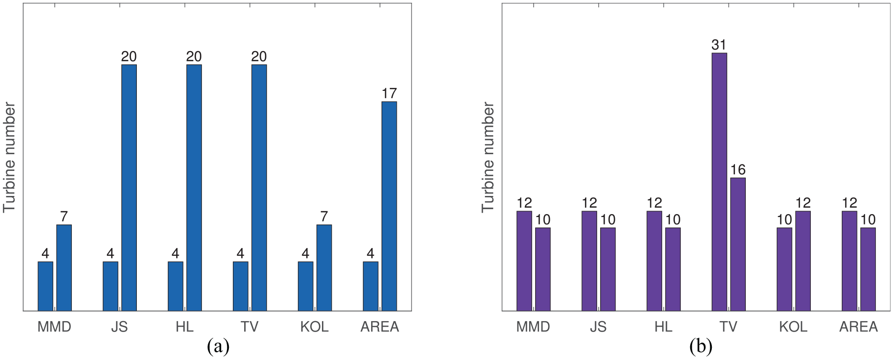
The two most dissimilar turbines from the confusion matrices when using absolute and normalised values are identified for each metric in Figure 19 by summing the difference values across all comparisons between turbines. Given the findings from earlier in this paper, these results should give an indication of the type of SHM features identified by the metric.
Most dissimilar turbines in the population when considering the brake-gear temperatures. (a) Absolute values and (b) self-standardised values.
Findings from the absolute case are:
According to Table 3, it is probable that T4, T7 and T20 stem from a global shift in mean, or a change in variance because the MMD, JS, HL and TV metrics prioritise those features over others. Indeed, Figures 18(a), 18(b) and 20(a) show that T4 and T7 are shifted in mean and T20 has a small variance.
- These shifts in mean of T4 and T7 are a result of the turbine’s position within the farm (T4 and T7 is located along one of the edges of the farm), and the speed and direction of the wind during this time period, suggesting that identifying signal shift via distance metrics may be useful for environmental mapping.
- The density function of T20 (Figure 20(a)), that drives these metrics, resembles the effects of decrease in amplitude from Figure 1. The temperature variation of T20 across the time period is smaller than others in the population (Figure 18(b)), possibly because of an operational issue; for example, the sensor may be damaged, consequently reducing its sensitivity to temperature changes. Clearly, automatically identifying this decrease in variance within the population would not be a simple task for a human. Given that three out of six metrics have detected this feature, this finding further supports the use of distance metrics for automated anomaly detection and suggests that they may be useful in detecting faults in the instrumentation.
•The Area metric identifies T17 as dissimilar, which could mean a shift in mean or a transient shift according to Table 3. Again, Figure 18(b) confirms that a transient shift has taken place in T17.
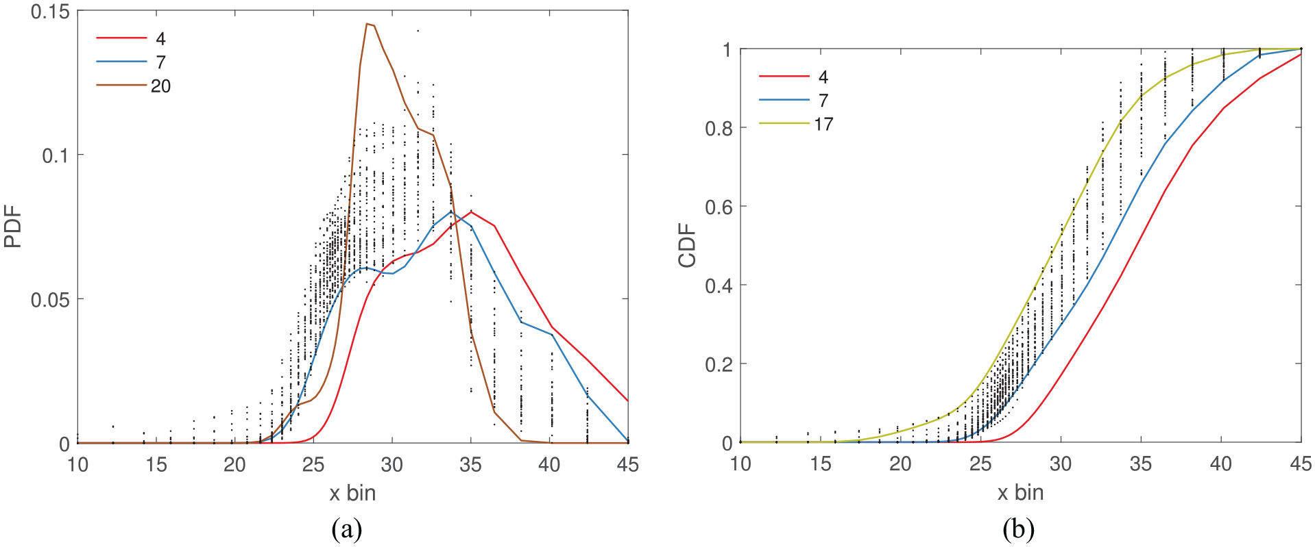
The density functions of the absolute data with the most dissimilar turbines highlighted. (a) Based on the PDF and (b) based on the CDF.
As expected from previous sections, when the data are standardised, T4 and T7 and T20 are no longer significantly dissimilar to the others, because the effects of translation and variance are diminished.
Insights from the standardised case are:
All metrics except TV identify T10 and T12 as the most dissimilar, suggesting from Table 4 that incremental shifts may be the cause. Figure 18(c) confirms that this is the case.
Surprisingly, the transient shifts of T17 are not highlighted by the metrics after self-standardisation, as expected from the results in Table 4. This result is because the transient shifts of other turbines (Figure 21(a)), are now more pronounced than that of T17.
Interestingly, the TV metric identifies different turbines (T16 and T31), to the other metrics as suggested by the findings from Table 4, possibly owing to small incremental shifts observed in Figure 18(d).
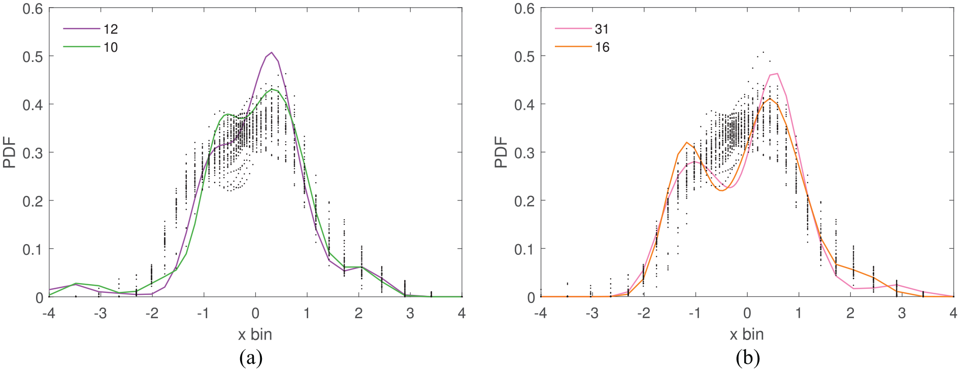
The density functions of the self-standardised data with the two most dissimilar turbines highlighted. (a) JS and HL normalised and (b) TV normalised.
The results presented in this section closely follow the findings from Sections ‘Distance metrics response to commonly occurring behaviours in SHM datasets’ and ‘Data normalisation and distance metrics’, validating the earlier findings and suggesting that the simulated dataset is suitable for evaluating the candidate distance metrics. As the general trend is similar across the population, only anomalous behaviours are identified easily and automatically.
The results from the case study indicate that a combination of HL, TV and Area metrics should help broaden the number of dissimilar turbines that can be identified from the dataset. Tables 3 and 4 also agree that these metrics prioritise a wide range of features. The most dissimilar turbines from each of these metrics across absolute and standardised data are highlighted in Figure 22(a). As the MMD negates the need for density estimation, and as it has a low overall score and variance in Figure 15, the most dissimilar turbines identified by the MMD are also presented in Figure 22(b). The combination of HL, TV and Area metrics find a large number of dissimilar turbines spanning many different features. The MMD performs relatively well, where it captures many of the same turbines. The recommendation is, therefore, to use a combination of HL, TV and Area metrics for a comprehensive dissimilarity identification and use the MMD to avoid the drawbacks of density estimation.
(a) The most dissimilar turbines identified by a combination of HL, TV, and Area giving a broad range of dissimilarities. When considering the the 10 most dissimilar turbines from the absolute and standardised cases, 13 turbines are identified by the three metrics and (b) the 10 most dissimilar turbines (from both absolute and standardised cases) identified by the MMD, a metric which has one of the best overall performances, without the need for density estimation. (a) TV, HL, Area and (b) MMD.
Conclusion
This is the first exploration of automated similarity assessment of feature data in population-based SHM, a new research field that aims to transfer knowledge across structures to address the shortcomings of SHM. PBSHM considers data from multiple structures and sensor networks, and therefore, new technologies are required to analyse vast amounts of data quickly and automatically, to aid positive transfer learning, and help identify suitable training and testing data. In this paper, distance metrics – that are not all widely used in SHM currently – were introduced in the context of PBSHM, and analysed for their ability to highlight similarity between members of the population at the top of the analysis chain, to aid the decision-making process.
Six distance metrics were tested on a simulated dataset, and on feature data collected from an operational wind farm, to evaluate their effectiveness at identifying commonly occurring features in PBSHM datasets. In both cases, the effect of data standardisation was also studied as it is a vital alignment step in transfer learning. The findings between the simulated and real datsets agreed and suggested that distance metrics are well suited for similarity assessment in PBSHM.
The results showed that most metrics were responsive to shifts in mean and variance when assessing absolute data, and transient effects when assessing standardised data. By assessing the response of the metrics to SHM features, it was found that a combination of metrics is required to identify a comprehensive variety of dissimilar behaviours within a population. The recommendations from the study are to use a combination of Hellinger, Total Variational (IPM form) and Area metrics to identify a broad range of dissimilarities in a population. If avoiding the drawbacks of density estimation is important, then the MMD is a useful metric, as it has a good response to all features evaluated.
These metrics are only suitable for use in large populations because the similarities (and, likewise, dissimilarities), are identified by comparison across the population. It is not possible to highlight dissimilarly behaving data from a structure using the distance metric value between itself and another structure. For these metrics to be used effectively, the population size should be large enough that it is possible to recognise the difference between data from a group of similarly behaving structures against a dissimilar structure.
In this paper, a homogeneous population of structures is studied, which reduces the complexity of assessing the similarity across the fleet, because the sensor network is also assumed to be similar across the population. However, it is entirely possible that small dissimilarities in the data will arise if some aspects of the sensor networks (sensor positions, types, manufacturers, models) are different across the population. This more complex case is the basis for transfer learning in PBSHM where knowledge transfer between source and target structures takes place where the behaviours of structures (and therefore the collected data) are different but related.
The metrics in this study were able to automatically identify numerous dissimilarities within absolute and standardised data, and give an indication of what type of features are present in the dataset without requiring manual inspection. Interestingly, the metrics detected some structures that behaved dissimilarly to the main population but behaved similarly to each other. As a consequence, it may be possible to group dissimilarly behaving structures in order to learn the mechanisms that drive these changes, or quickly find associations when analysing new data that may have similar trends. Overall, the use of distance metrics was found to be extremely helpful for PBSHM, and is likely to be advantageous to other systems concerned with fleet management.
Footnotes
Acknowledgements
This work has been supported by the UK Engineering and Physical Sciences Research Council (EPSRC), via the project A New Partnership in Offshore Wind (grant numbers EP/K003836/2, and EP/R004900/1). K.W. also gratefully acknowledges support from the EPSRC via grant no. EP/J016942/1 and E.J.C. is grateful to EPSRC for support via grant no. EP/S001565/1. The authors would also like to thank Vattenfall for providing the data used for this work. For the purpose of open access, the author has applied a Creative Commons Attribution (CC BY) licence to any Author Accepted Manuscript version arising.
Declaration of conflicting interests
The author(s) declared no potential conflicts of interest with respect to the research, authorship, and/or publication of this article.
Funding
The author(s) disclosed receipt of the following financial support for the research, authorship, and/or publication of this article: This research was supported by grants from the UK Engineering and Physical Sciences Research Council (EP/K003836/2, EP/R004900/1, EP/J016942/1, EP/S001565/1). The funder had no role in study design, data collection and analysis, decision to publish, or preparation of the manuscript.