
Abstract
There are few studies on the fault diagnosis of deep learning in real large-scale bearings, such as wind turbine pitch bearings. We present a novel fault diagnosis method, Bayesian augmented temporal convolutional network (BATCN), to filter the raw signal in wind turbine pitch bearing defect detection. This method, which employs temporal convolutional neural networks, is designed to capture the temporal dependencies of the signal, with such a focus on non-stationary relationships in the collected signals. By referring to the thoughts of Bayesian optimization, our approach can spontaneously find the best patch length that influences fault signal extraction during the filtering process, avoiding manual tuning of this hyper-parameter. This BATCN method is first performed on simulation signals and an open-source dataset of general bearings, and then validated on industrial wind turbine pitch bearings both in the lab and in the real wind farm, where the bearings have been operated for over 15 years. The results show that our method can work well for large-scale slow-speed wind turbine pitch bearings.
Keywords
Introduction
Wind power, as a sustainable and reliable energy source,1,2 its installation capacity has expanded at a predominant pace in recent years throughout the world, and this trend is expected to continue constantly in order to achieve carbon emission target in 2050 and provide sustainable electric energy. 3 Pitch bearings, also referred to as blade bearings, one of the most significant components of wind turbines, can improve the generating efficiency and ensure the safe operation of wind turbine systems.4,5 However, the extreme operating conditions in industrial occasions may result in serious faults, along with catastrophic accidents and significant financial losses.6,7 Therefore, Condition Monitoring and Fault Diagnosis (CMFD) 8 of wind turbine pitch bearings driven by measured data is one of the feasible solutions for guaranteeing reliability and controlling maintenance costs. 9 In the CMFD, the vibration or acoustic signal can be used as the fundamental unit to diagnose the faults existing in bearings.10,11
When faults occur in bearings, they often generate periodic or quasi-periodic fault signals. 12 However, fault signals are weak under slow-speed conditions because low rotation results in little kinetic energy, owing to Newton’s law. In addition, weak fault signals are often masked by background noise (from natural distractions) and harmonic interference (from bearing rotation, gearbox, and motor driving). 13 For the reasons mentioned above, fault signals in wind turbine pitch bearings are usually challenging to be extracted from collected raw signals.
Over the last few decades, some classical denoising methods have been proposed for filtering signals to extract fault signals. The discrete/random separation method15,16 filters raw signals by eliminating the periodic property in the time domain. The spectral kurtosis (SK) method 17 directly extracts fault signals in a narrow frequency band by finding the best central frequency and band width with the aim of determining the best inverse filter. 18 Some researchers recently have also focused on other potential approaches in bearing defect diagnosis, like dictionary methods and statistical methods. Regarding dictionary methods, Bayesian- and Lagrangian-based methods were proposed to construct a noise dictionary for collected raw signals. 19 The correlation filtering approach was used to create an adaptive over-complete dictionary using the unit impulse response function. 20 As for statistical methods, Guo et al. 21 used the matrix decomposition method k-means singular value decomposition for defect detection of wind turbine bearings. Aye et al. 22 used the principal component analysis (PCA) approach to gently identify bearing degradation under varied slow-speed situations.
In recent years, the deep learning techniques, especially convolutional neural networks (CNNs),23,24 have attracted significant research attention on rolling bearing fault detection. Zhang et al. 25 integrated the function of the PCA into CNN to process the fault signals from multidimensional bearing vibration signals. Chen et al. 26 researched a transfer learning to augment CNN so that the experience in bearing and gear faults can be reused. Li et al. 27 investigated a novel wavelet-driven deep neural network of using the wavelet kernels in the first network layer so that it can offer CNN the ability to discover weak fault signals of gearbox. Kumar et al. 28 apply a sparsity CNN to diagnose bearing faults under the condition of limited training samples.
Currently, most of the deep learning methods are designed for direct fault classification and judgement. Only few work is related to direct signal denoising of vibration signals from bearings. Wang et al. 29 proposed a novel joint learning CNN for bearing condition monitoring. This method is divided into fault diagnosis and signal denoising module, which can obtain good noise robustness through the decoupling functional modules. In the signal denoising module, the encoder–decoder network structure is utilized, attention-based encoder for useful fault signals and decoder for recovering signal details. This method is validated with excellent signal denoising performance. Although this work studied the signal denoising for mechanical bearings with deep learning techniques, large-scale mechanical rotating bearings (such as wind turbine bearings) with special noise levels due to friction and collision between different components has not been studied. This part of the research gap needs to be filled.
Additionally, a seemingly insurmountable technical problem of determining the patch length may exist in the signal processing during the fault diagnosis process. The patch length during the processing of vibration signals is a key factor influencing the processing performance. The deep learning method considering the input patch length was used for intelligent fault diagnosis of rolling bearings in the study by Li et al., 30 but suitable patch length was only given by some trials. The one-dimensional signals is split with fixed patch length, and the determination of patch length can be ignored by the subsequent processing of transformer encoder in the study by Pei et al. 31 However, this is just another way indirectly thinking about patch length. The fault pluse extraction can be realized by dictionary learning method in the study by Chen et al., 32 but the patch length in this work was only given by empirical setting.
On top of the aforementioned challenges, there are some open challenges in the field of wind turbine pitch bearing fault diagnosis. More specifically, wind turbine pitch bearing is operated under oscillating operating speed, leading to non-stationary fault signals. Although the existing filtering methods for constant rotating speed can still be applied, the performance may be limited when the fault signal is weak or harmonic interference (e.g. introduced by driving rotor and gear) strongly couples with fault frequency (FF) band. Furthermore, vibration-based fault detection often requires high sampling frequency, producing large amount of data and redundant information. This introduces high computational loading when using complex filtering methods, such as deep neural networks.
This paper proposed a robust denoising method that can be applied for collected signals to realize fault diagnosis of wind turbine pitch bearing. It is the first time to use CNN for wind turbine pitch bearing fault extraction. This method utilizes the strong feature extraction capability of convolutional networks to process collected discrete signals consisting of much redundant information. We proposed a new fault diagnosis method, called Bayesian augmented temporal convolutional networks (BATCN), to detect defects in wind turbine pitch bearings. The BATCN method, using deep learning techniques, can learn the intrinsic features of fault signals to guarantee the extraction of non-stationary fault signals. The proposed BATCN method learned not only the fault signal and period information but also the dependency relationship among different time intervals, so that it can deal with the non-stationary signals well. By employing global characteristics of convolutional networks, the BATCN also has the ability of harmonic interference suppression. In addition, the dilated convolution in BATCN can realize the sparsity so that the computation complexity can be reduced, to a large extent. Referring to Bayesian optimization, our approach can spontaneously find the best patch length in the BATCN method so that the proposed method can perform well without complex adjusting parameters.
Regarding the research design, it can explain the work of this article from another perspective. Specifically, the classic SK method has been repeatedly demonstrated to be very effective in general bearing signal denoising, so it will be used as the primary comparing method in this article. Unlike the processing complexity for image and video streaming, the one-dimensional signals are relatively straightforward, so the CNN may be sufficiently effective and hence are the focus of this article.
Combined with the foregoing design analysis, the primary contributions of this article can therefore be summarized as follows:
This article proposes a novel method called BATCN of using the CNN technique to denoise the signals of wind turbine pitch bearings, which can achieve excellent filtering performance without adjusting patch length.
This is presumably the first study to verify that deep learning can improve the denoising performance of wind turbine pitch bearings. Compared with the classical SK method, the deep learning method is proved more effectively in some conditions of the wind turbine pitch bearings.
The rest of this work is laid out as follows: the section ‘Fault diagnosis’ is dedicated to the complete fault diagnosis procedure for wind turbine pitch bearings and some prior knowledge on fault diagnosis. In the section ‘Denoising BATCN method’, the theoretical process of proposed BATCN is explained in detail. The section ‘Simulation validation’ uses two simulations to validate the noise suppression and harmonic interference suppression, respectively. The section ‘Physical experiments’ subsequently presents experimental comparisons between the proposed BATCN approach and the classical SK approach. The section ‘Meta-analysis’ shows the meta-analysis of the proposed method, and the section ‘Conclusion’ concludes the work in this article.
Fault diagnosis
This section would present the complete fault diagnosis procedure for wind turbine pitch bearings, which could be divided into two procedures: signal filter and fault inference. Firstly, the signal filter procedure would utilize BATCN to filter raw acoustic emission signals and then get denoised signals. Subsequently, fault inference would calculate the FF to identify corresponding fault type by envelope signals. Figure 1 shows the concrete procedures.
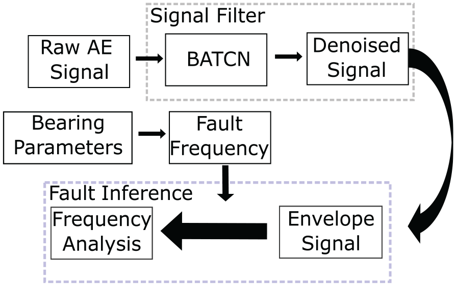
Procedures of fault diagnosis.
The following section would briefly explain the FF and envelope techniques used in this article. The FF is a key parameter used to identify the type of fault during the frequency analysis process. Through frequency analysis, characteristic information such as the FF can be obtained, allowing defects to be accurately identified based on the calculated FF. 33 The FF could be obtained by equation (1).
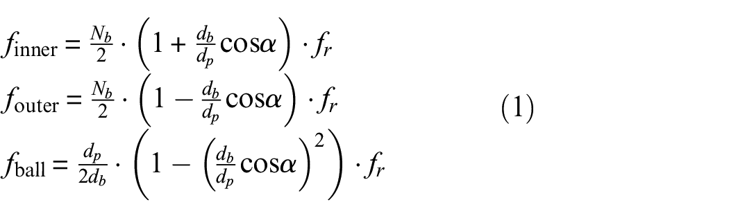
where
With regard to the envelope processing, this article focuses exclusively on the use of the Hilbert transform. By utilizing the complex signal, the envelope and phase can be calculated conveniently. However, it should be noted that all signals collected from natural sources are real signals, and the complex signals could not be obtained directly. Therefore, the Hilbert transform is used to construct complex signals for the purposes of envelope processing. This could also be called Hilbert envelope.
Denoising BATCN method
The architecture of proposed BATCN is illustrated in Figure 2. It is worth noting that the feature extraction module in BATCN refers to a type of parallel method called temporal CNNs. In addition, this proposed BATCN method utilizes Bayesian optimization to find the optimal patch length to filter signals better. Meanwhile, the forward and backward sequences are processed by encoder 1 and encoder 2, respectively, both of which are made up of fully connected layers. The decoder calculates the goal using the training loss output from the encoders and the kurtosis information of signals so that the exploration function may determine the next exploring location. The Gaussian process (GP) can be used as a surrogate model in this case.
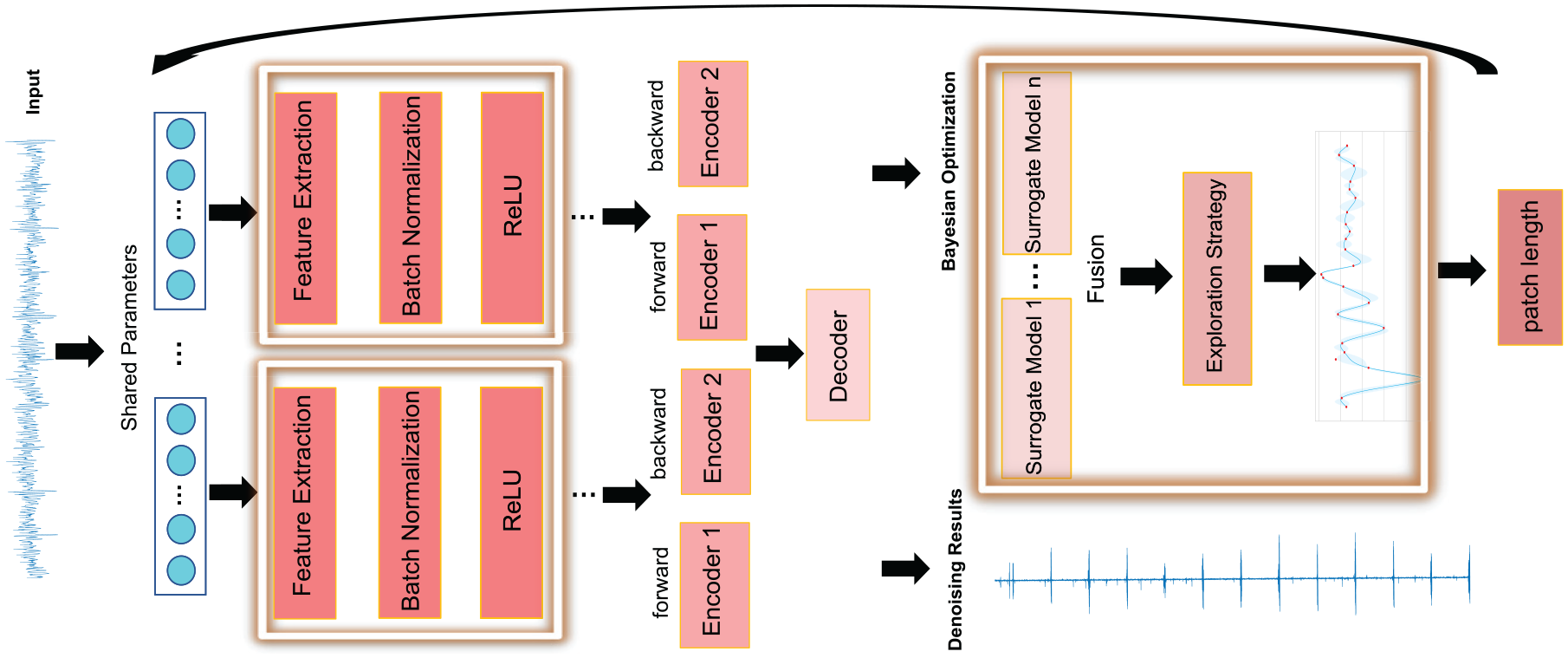
BATCN structure.
Feature extraction module
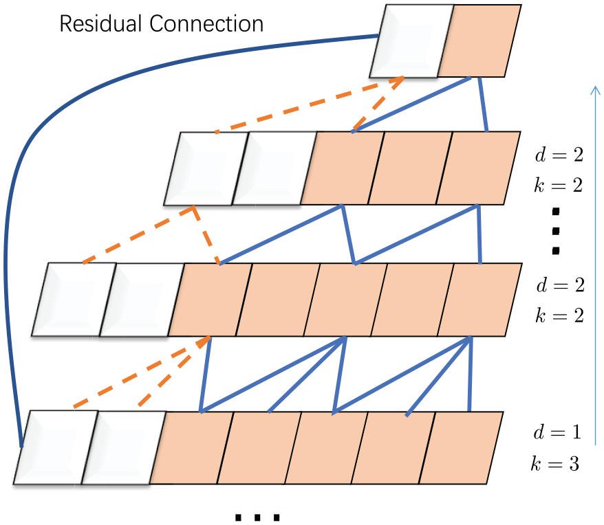
This feature extraction module in the BATCN method includes three segments: causal convolutions, dilated convolutions and residual connections. Figure 3 demonstrates the architecture of feature extraction, which processes the discrete sequences of input.
Feature extraction module.
Causal convolutions
To obtain characteristic information from unidentified sequence data, causal convolution is applied, inspired by the fully convolutional networks. 34 Utilizing causal convolutions, the realistic data derived from low-layer convolution operations can be transmitted to the high layer with abstract form. The information in the higher layers becomes increasingly intensive until the projected value is output in the top layer, as illustrated in Figure 3.
The causal convolutions describe the relationship between two adjacent layers. Assume input vector of the previous layer

where
Dilated convolutions
Although causal convolutions can extract feature information well, this may still generate deep networks with many layers. According to study, 35 dilated convolution may be used to minimize the depth of neural networks by extending the receptive field. When the input size is known, dilated convolution refers to a longer history than ordinary causal convolution, resulting in fewer convolution operations and a reduction in the number of layers necessary for a neural network.
For the sequence data input vector
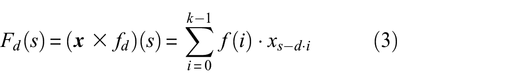
where
Residual connection
The neural networks are still deep, despite the use of dilated convolutions, resulting in awful training loss curve. To minimize performance degradation from deep networks, a residual connection
36
developed for image processing may also be used for sequence data processing. When compared to the standard output

Here, the input and output of the current layer are
Determination of patch length with Bayesian optimization
Before training the neural networks, the patch length, also referred to as the input size for the training dataset, is crucial for denoising performance. For signal sequence data
To some extent, the patch length during model construction is a factor that will influence the performance of denoising models. However, trial-and-error methods, such as enumeration method, are unrealistic because every single training session is very time-consuming. The aimless search may not be suitable for this occasion, so a Bayesian optimization-based search strategy is used for finding the best patch length automatically.
Search process for patch length
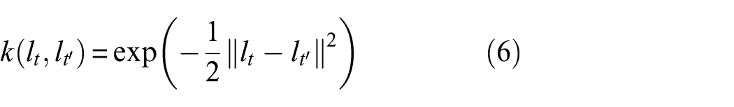
It is assumed that

where the
Subsequently, the Sherman–Morrison–Woodbury formula
39
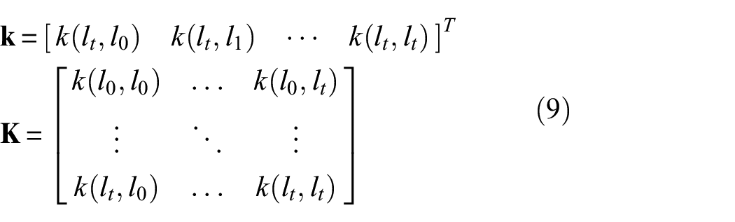
can be used to generate a predictive distribution

where
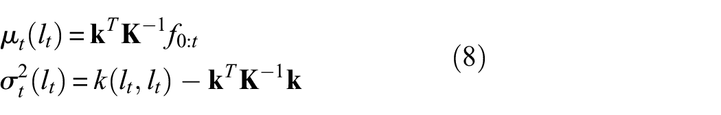
where
According to equation (7), the GP can be updated:

From equations (5) to (10), we can identify the procedures of updating the GP. Furthermore, the acquisition function for choosing the next point needs to be concretely explained.
Some acquisition functions related to the exploration approach have been empirically identified as effective on most occasions. The three primary acquisition functions are explained as follows:
Upper confidence bound (UCB):

where
Probability of improvement (PI):
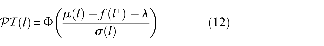
where
Expected improvement (EI):

where
Regarding selection of acquisition function, global search for UCB is simple, but convergence speed is slow. PI can quickly converge, but it is possible to become stuck in a locally optimum solution. EI is able to find a balance between global and local optimization.
Finally, we select EI acquisition function as the exploration strategy because it will make trade-off between global optimization and local search.
Simulation validation
Noise and harmonic interference are significant factors that may influence the fault diagnosis of wind turbine pitch bearings. This section firstly introduce simulation signals, including: fault signals, harmonic signals and noise signals. Subsequently, noise and harmonic interference suppression of the proposed BATCN method will be examined, respectively. In addition, SK, 17 a denoising approach that has been proven to be effective in a variety of general bearing applications, was used for comparison.
Simulated signals
The simulation signal is comprised of three parts: fault signals
Fault signals
At time
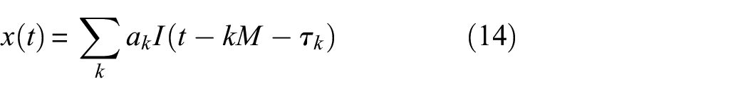
The standard form of
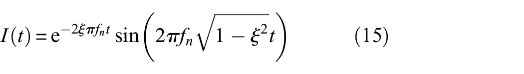
where different
Harmonic signals
To effectively test the ability of harmonic interference suppression, the harmonic signals
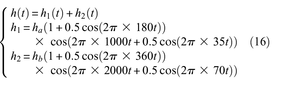
where
Noise signals
The noise signals are also significant to guarantee the integrity of simulated signals, shown as follows:
where the nature of
Indicators
To measure various interferences, three indicators, signal-to-noise ratio (SNR), signal-to-harmonic ratio (SHR) and signal-to-interference ratio (SIR), were introduced, respectively:
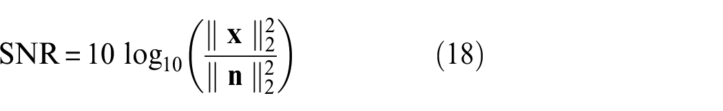
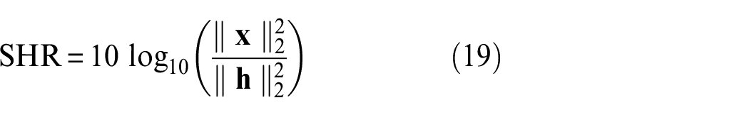
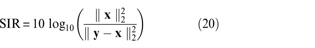
where
Additionally, to evaluate the denoising performance, kurtosis value is introduced by following. 40 Kurtosis measures the flatness of data distribution, and it is the statistics of the degree of steepness of data distribution morphology. The large kurtosis values often denote good denoising results.
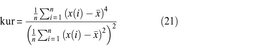
where
Noise suppression performance
The collected raw signals from real world are often mingled with random noise signals, indicating that noise suppression is necessary for a fault diagnosis method.
To evaluate noise suppression, a comparison is made between the classical SK method and the proposed BATCN method. The simulated signal to be tested comprises both noise and fault signals, with the following parameter settings.
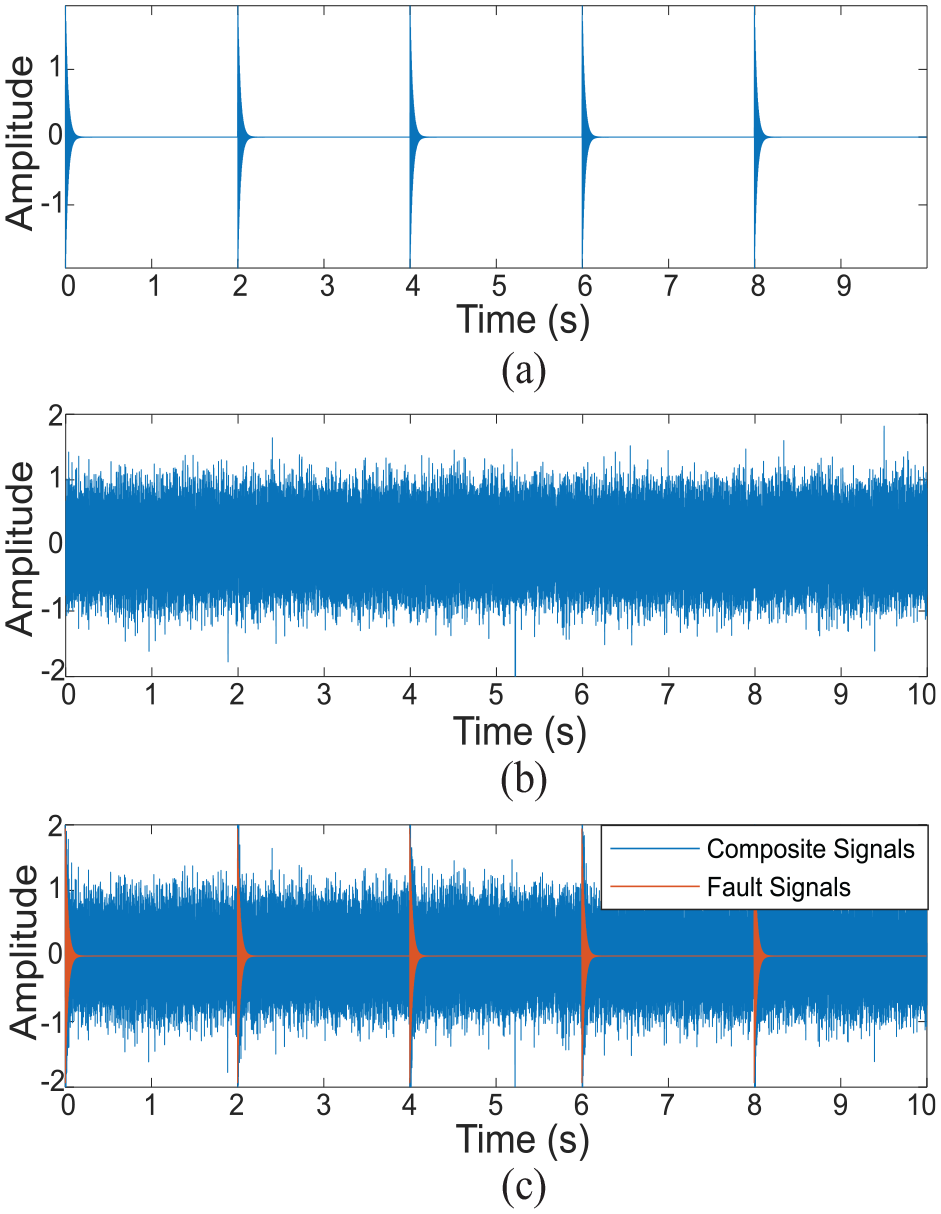
Constructing simulation signals for noise suppression test (a) simulated fault signals with kurtosis of 101.78, (b) simulated noise signals with kurtosis of 2.98 and (c) composited signals with SNR −10.01 dB, kurtosis of 3.77.
Figure 5 shows the comparison results of noise suppression. The SK denoised results in Figure 5(a) show that the profile of the fault signals can be seen in the time domain. When compared to composite signals, the kurtosis increased from 3.77 to 10.25, indicating that the classical SK method is effective in eliminating general noise, but low amplitude noise redundancy persists. The BATCN denoised results in Figure 5(b) show that the noise can be almost fully reduced, and the filtered signals have a large kurtosis of 1363.46. The results from this simulated example shows that the BATCN method has better noise suppression ability than the SK method.
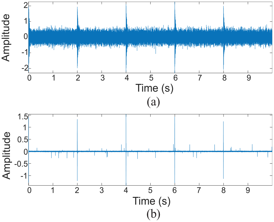
Noise suppression evaluation (a) SK filtered signals with kurtosis of 10.25 and (b) BATCN filtered signals with kurtosis of 1363.46.
Harmonic interference suppression performance
Harmonic interference from rotor rotating and gear meshing may make difficult to recognize fault characteristic frequency. To examine harmonic interference suppression, the SK method is also used to compare the proposed BATCN method.
The simulation parameters are set as follows:
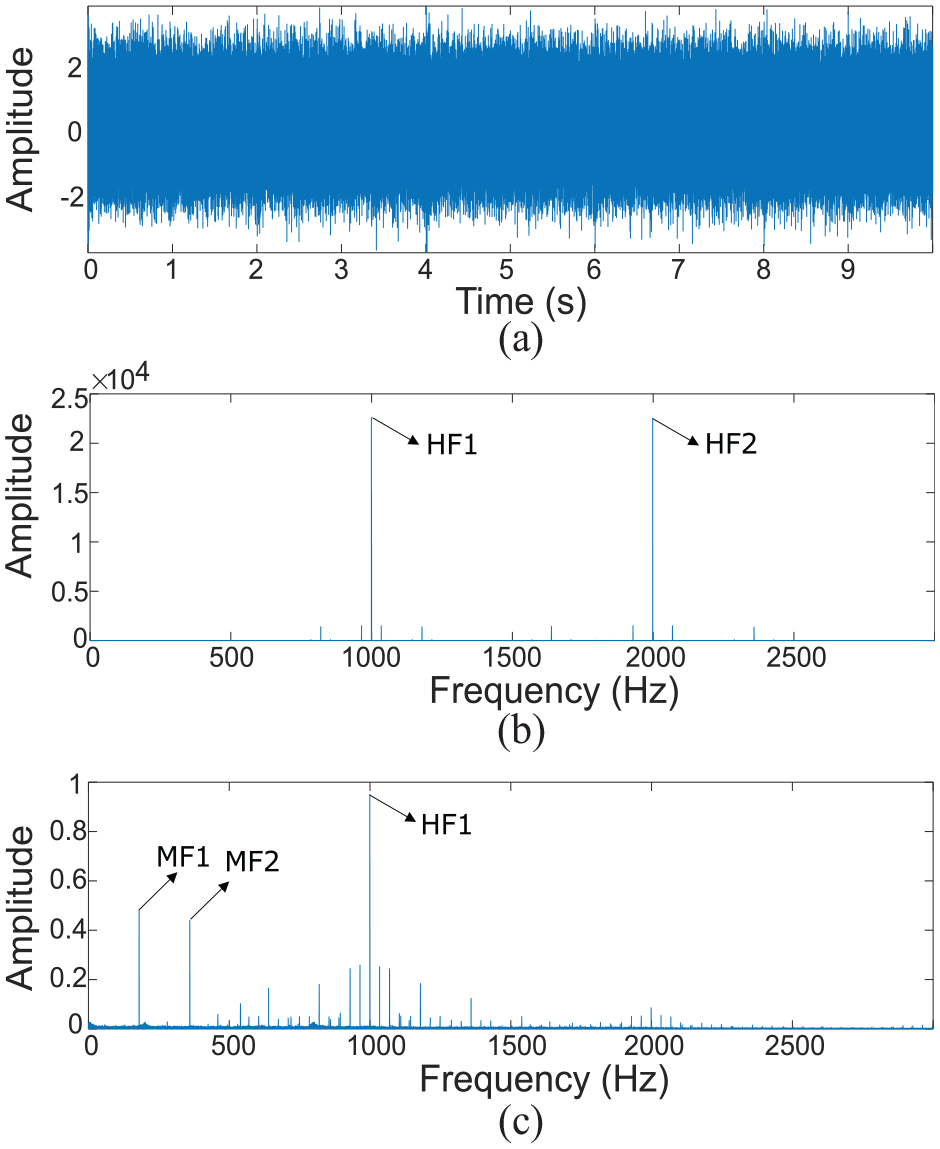
Harmonic interference suppression evaluation without any denoising method (a) time domain, (b) frequency domain and (c) Hilbert envelope spectrum.
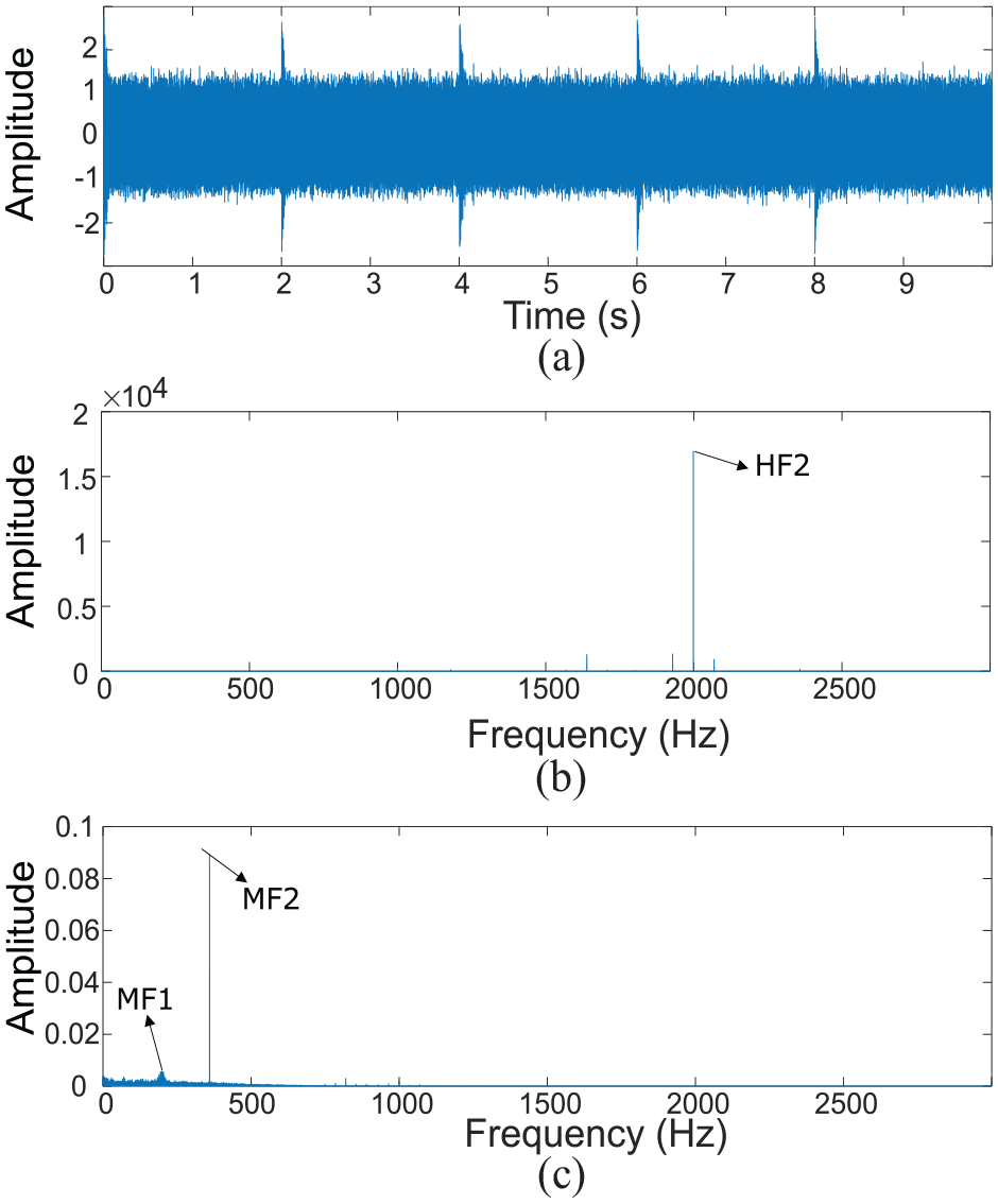
Figure 7 actually shows three sub-figures, labelled as (a), (b) and (c), respectively. Figure 7(a) shows the time-domain signal after the processing of the SK method, where the profile of fault signals can be observed. Figure 7(b) shows the frequency spectrum after the SK method, where the dominant frequency component is still HF2. Figure 7(c) shows the frequency spectrum after the Hilbert envelope, where the modulation frequencies MF1 and MF2 are still obvious.
Harmonic interference suppression evaluation with the SK method (a) time domain, (b) frequency domain and (c) Hilbert envelope spectrum.
In Figure 8(b), the RF can be observed in frequency domain after using the proposed BATCN method. Additionally, all the HF, MF and RF are submerged in Hilbert envelop spectrum, as shown in Figure 8(c). Meanwhile, the FF can be observed clearly through enlargement. Through comparisons between SK and BATCN results, it can be concluded that BATCN can effectively extract fault signals and detect FF due to the significant advantage of harmonic interference suppression.
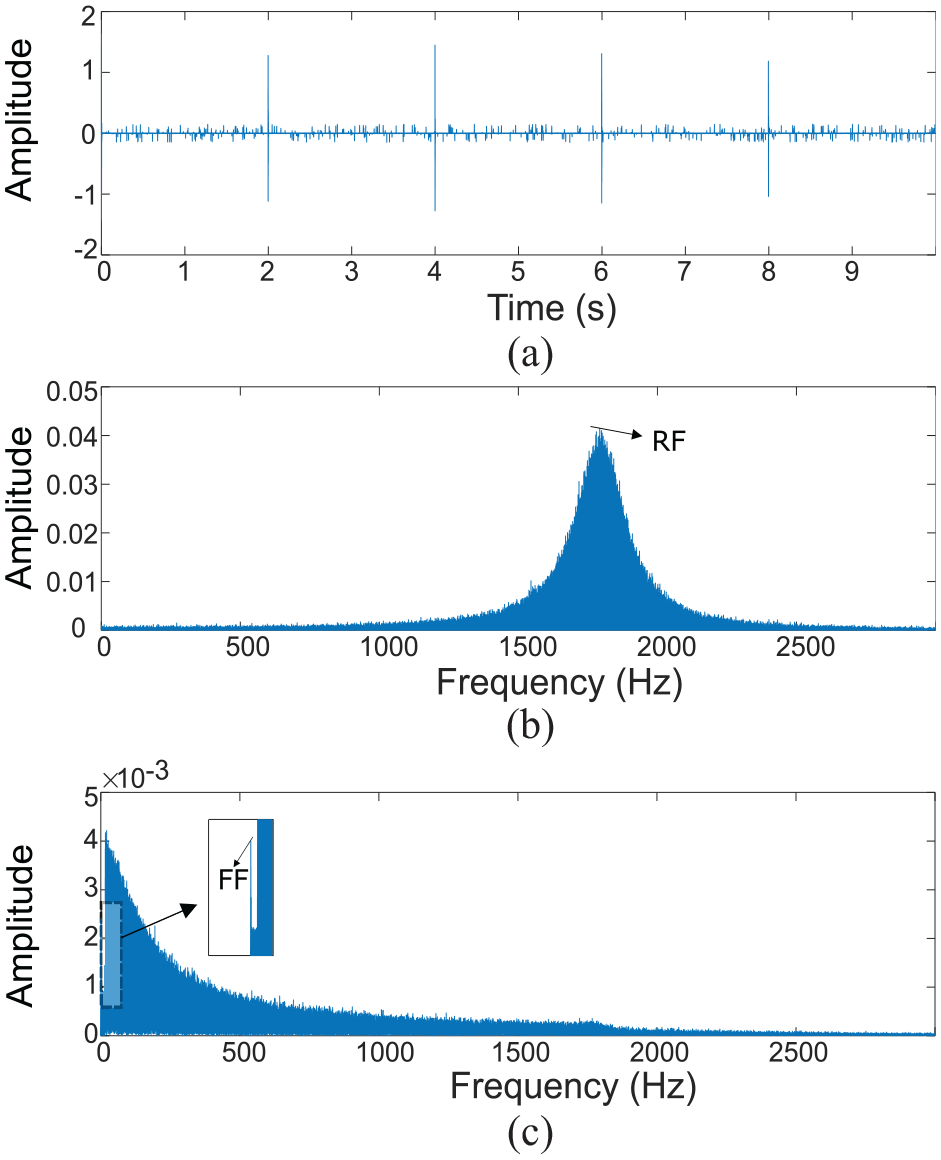
Harmonic interference suppression evaluation with the BATCN method (a) time domain, (b) frequency domain and (c) Hilbert envelope spectrum.
Physical experiments
This section uses three physical cases to test the proposed BATCN method. Data in case 1 are from a public dataset Machinery Failure Prevention Technology (MFPT) ([Online], available: https://github.com/mathworks/RollingElementBearingFaultDiagnosis-Data). Data in case 2 are collected in a lab environment from wind turbine pitch bearings that have been serviced for 15 years in real-world wind farms. Data in case 3 are obtained from a field wind turbine in a real-world wind farm but is known to work abnormally.
Case 1
This case here is related to an open-source dataset, MFPT, that is collected in general bearing with sampling frequency 48,828 Hz. MFPT dataset contains two fault types, inner fault (case 1.1) and outer fault (case 1.2). The corresponding FFs of the inner fault and outer fault are named ballpass frequency inner race (BPFI) and ballpass frequency outer race (BPFO), respectively. We first test the proposed BATCN method in MFPT general bearing (case 1), and then method validation for real-world wind turbine pitch bearing will be subsequently executed in case 2 and case 3. Figure 9 is the analysis results for normal bearing. From Figure 9(d) or (e), it can observe that we cannot identify any FF. Figures 10 and 11 represent the damaged conditions, with inner fault and outer fault, respectively.
MFPT normal bearing (a) raw signals, (b) SK denoised signals, (c) BATCN denoised signals, (d) Hilbert envelope spectrum based on SK denoised signals and (e) Hilbert envelope spectrum based on BATCN denoised signals.
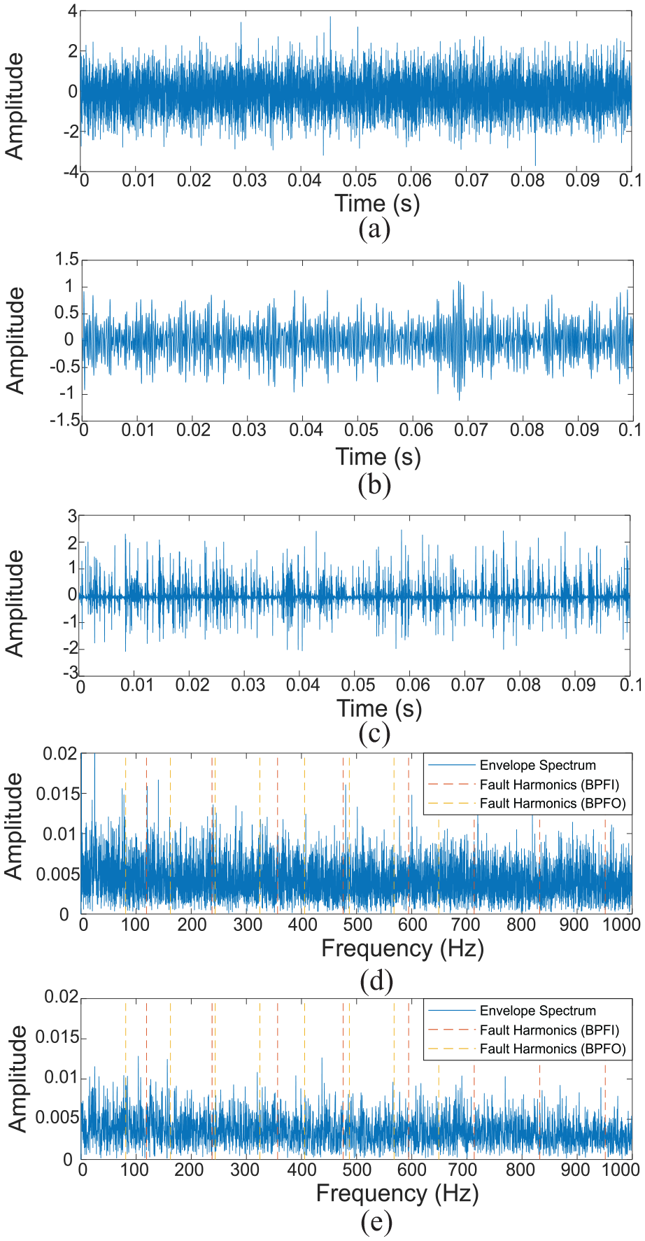
MFPT inner fault bearing, case 1.1 (a) raw signals, (b) SK denoised signals, (c) BATCN denoised signals, (d) Hilbert envelope spectrum based on SK denoised signals and (e) Hilbert envelope spectrum based on BATCN denoised signals.
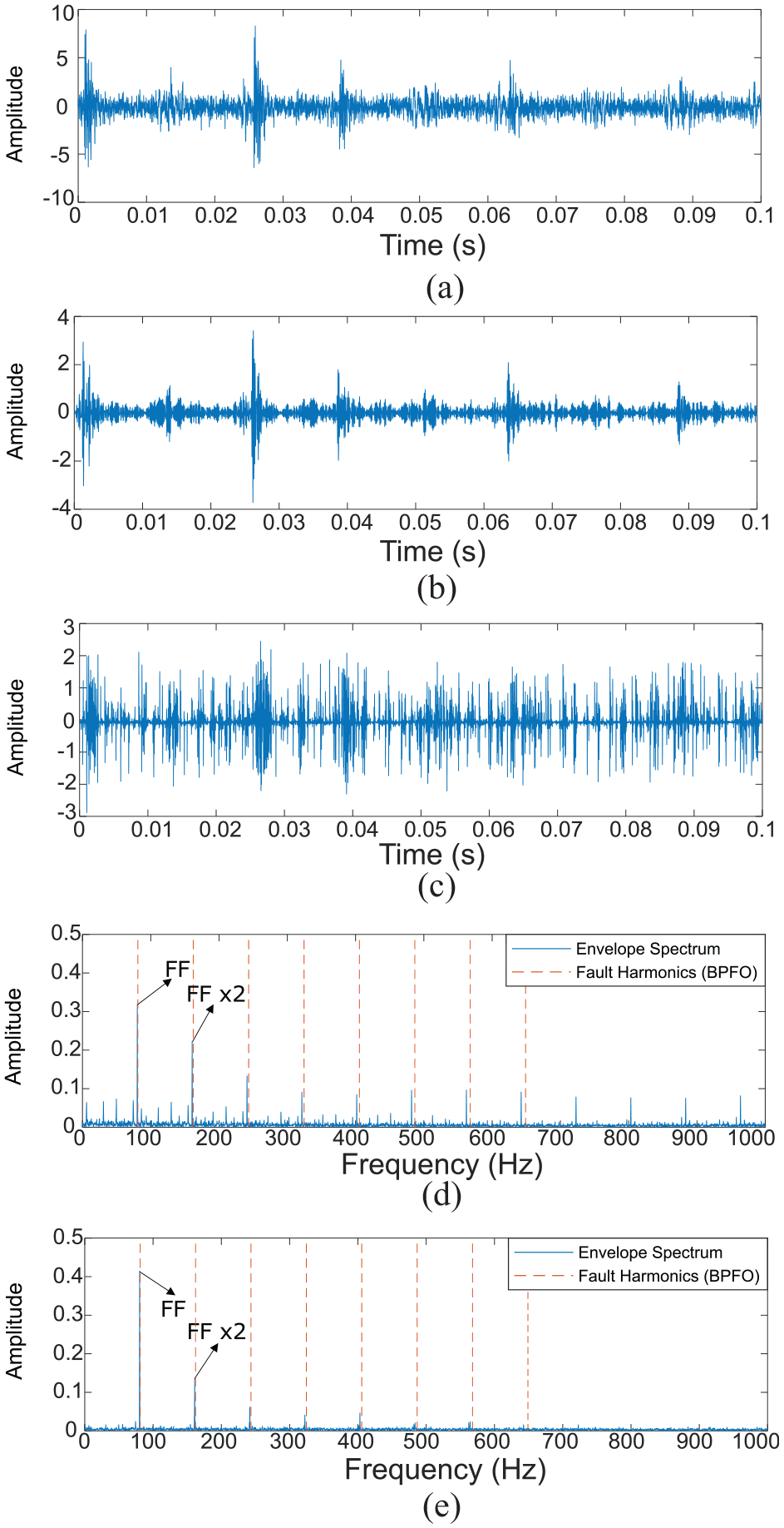
MFPT outer fault bearing, case 1.2 (a) raw signals, (b) SK denoised signals, (c) BATCN denoised signals, (d) Hilbert envelope spectrum based on SK denoised signals and (e) Hilbert envelope spectrum based on BATCN denoised signals.
As can be seen in Figure 10, when using the SK method to filter the raw signal with inner fault, the Hilbert envelope spectrum Figure 10(d) may still exist some interference frequency. However, the BATCN filtered signal can clearly identify FF in its Hilbert envelope spectrum Figure 10(e). In addition, using the BATCN method, higher fault harmonic components in the envelope spectrum seem to decay quickly.
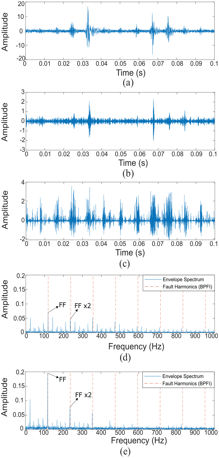
By observing Figure 11, we can draw similar conclusions to those of Figure 10. One notable point in these conclusions is that the higher fault harmonic components present in the envelope spectrum also exhibit a rapid reduction. This phenomenon is more significant for slow-speed bearings, such as wind turbine pitch bearings, because the higher fault harmonics in the slow-speed condition may overlap with other types of FF and make it challenging to identify the correct FF. To quantitatively compare the performance between SK and BATCN, we can define amplitude of corresponding frequency in Hilbert envelope spectrum as AMP. FF*1 is FF, FF*2 and FF*5 represent FF times 2 and 5, respectively. As shown in Table 1, BATCN has the larger amplitude at FF*1 frequency than SK. Regarding the large FF*2/FF*1 and FF*5/FF*1 for BATCN, indicating that the fault harmonics decay more rapidly in the Hilbert envelope spectrum of the BATCN method, which is advantageous for fault diagnosis.
Case 1: quantitative results of signals processed by SK and BATCN.
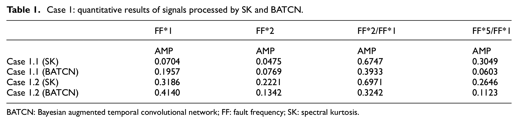
BATCN: Bayesian augmented temporal convolutional network; FF: fault frequency; SK: spectral kurtosis.
Case 2
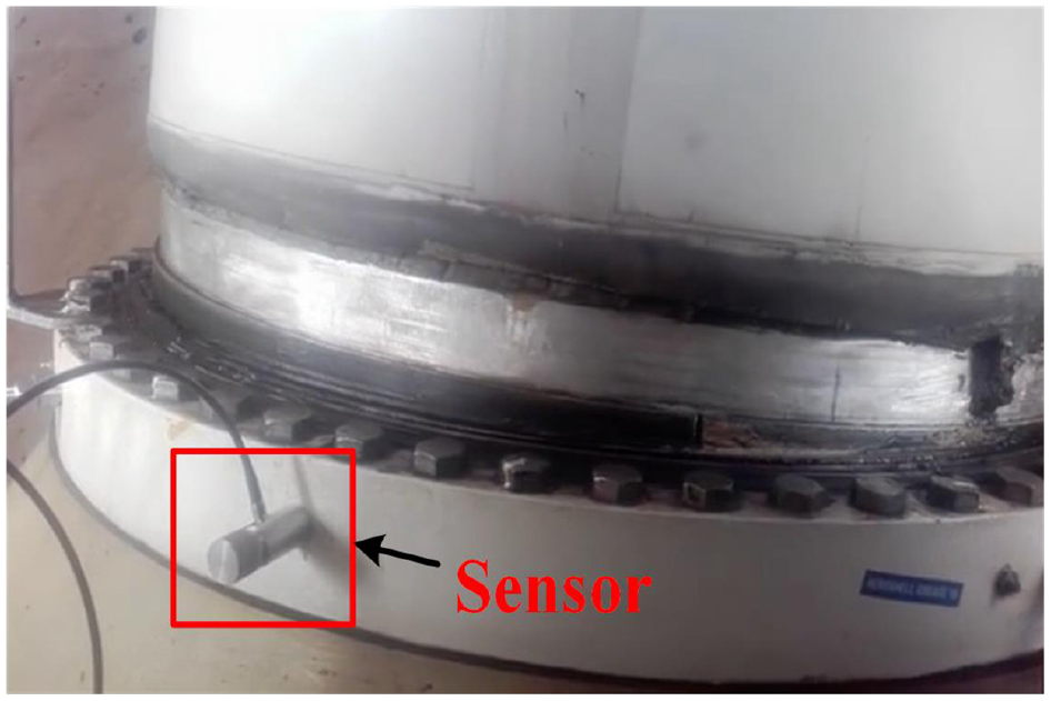
The data, in this case, are collected from the industrial-scale wind turbine bearing lab at the University of Manchester. The bearings have been operated in a real-world wind farm for over 15 years and have naturally incurred defects. The bearings have a diameter of 1 m and a mass of 261 kg. The sampling frequency is initially chosen as 100 kHz. This high sampling frequency produces significant computational demands on the proposed method. Therefore, the collected data are downsampled to 1 kHz. In this case, this proposed method only needs low computations while maintaining good filtering and fault diagnosis abilities. The case 2.1 is executed without loadings. The case 2.2 is operated with loadings, which may result in a little bit rotating speed fluctuation. The left and front views of the test rig are shown in Figure 12(a) and (b), respectively. Table 2 describes the three types of FF of the wind turbine pitch bearing, and the FF in this case is the inner FF, namely BPFI.
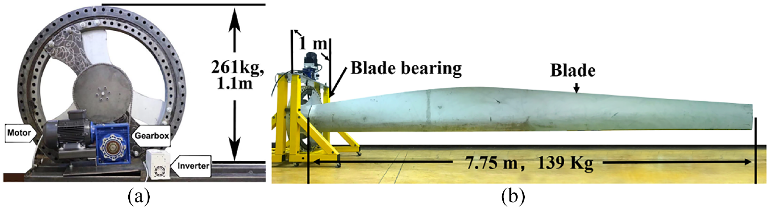
View of test rig (a) left view and (b) front view.
Theoretical FF of the wind turbine pitch bearing.
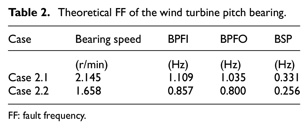
FF: fault frequency.
On top of the SK method, the TCN method is also added to compare with our proposed BATCN method. Figures 13 and 14 compare different methods in the time and frequency domains for case 2.1, whereas Figures 15 and 16 do the same for case 2.2. Observing the magnified time-domain plot in Figures 13 and 15, it can be observed that, compared to other methods, BATCN demonstrates a better ability to extract fault signals. Observing the frequency-domain results in Figures 14 and 16, it can be found that compared to other methods, BATCN can better extract the characteristic frequencies of the FF and double FF (FF*2), and the FF is more obvious compared to other orders of FF.
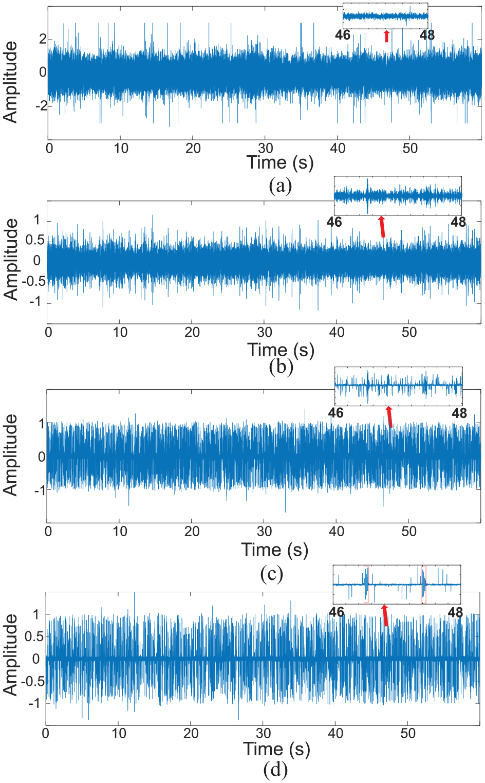
Laboratorial wind turbine pitch bearing fault, case 2.1 (a) raw signals, (b) SK denoised signals, (c) TCN denoised signals and (d) BATCN denoised signals.
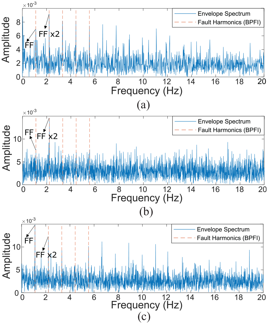
Laboratorial wind turbine pitch bearing fault, case 2.1 (a) Hilbert envelope spectrum based on SK denoised signals, (b) Hilbert envelope spectrum based on TCN denoised signals and (c) Hilbert envelope spectrum based on BATCN denoised signals.
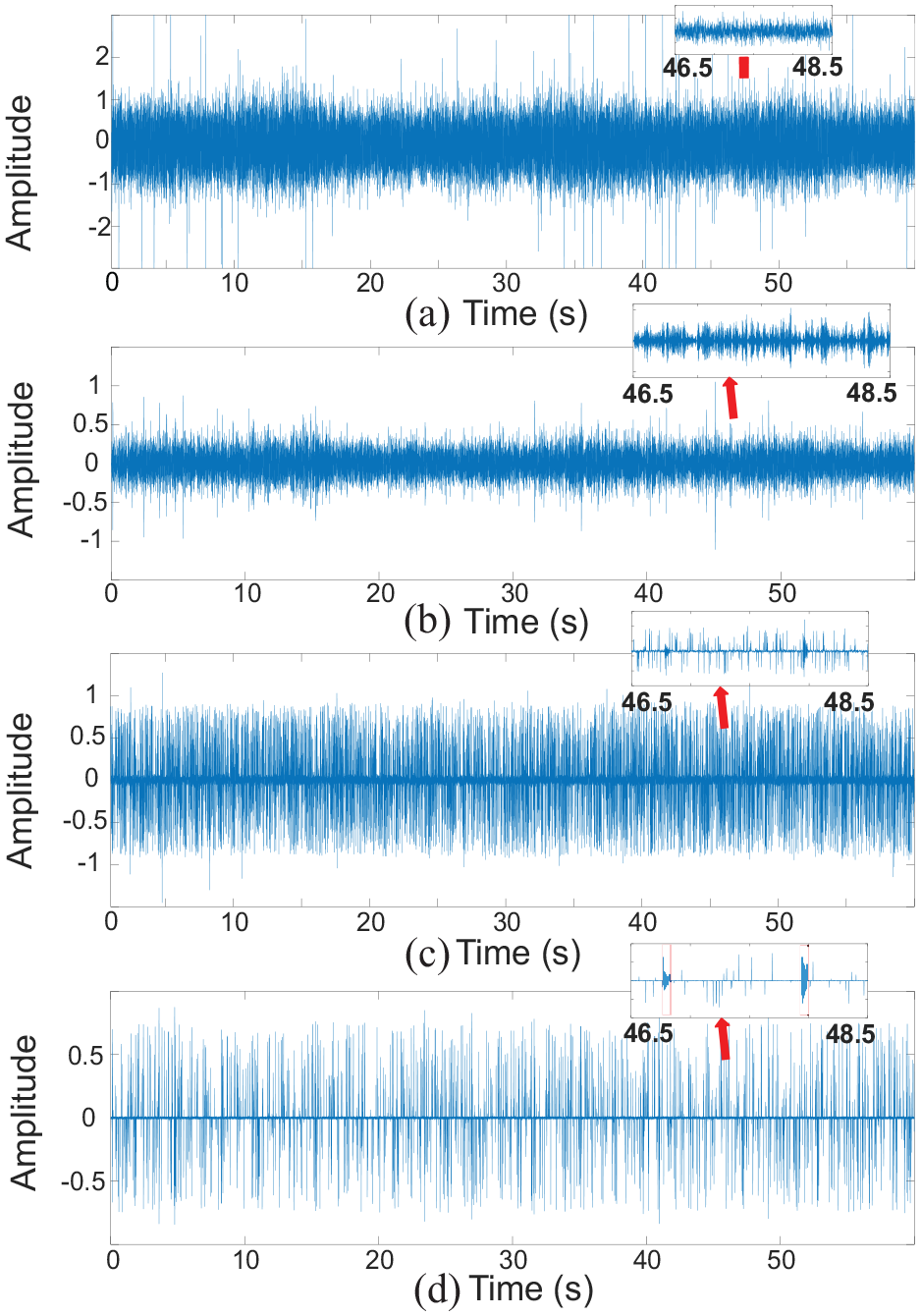
Laboratorial wind turbine pitch bearing fault, case 2.2 (a) raw signals, (b) SK denoised signals, (c) TCN denoised signals and (d) BATCN denoised signals.

Laboratorial wind turbine pitch bearing fault, case 2.2 (a) Hilbert envelope spectrum based on SK denoised signals, (b) Hilbert envelope spectrum based on TCN denoised signals and (c) Hilbert envelope spectrum based on BATCN denoised signals.
To quantitatively compare the performance between SK and BATCN, we can define amplitude of corresponding frequency in Hilbert envelope spectrum as AMP. FF*1 is FF, FF*2 and FF*5 are FF times 2 and 5, respectively. As shown in Table 3, the BATCN can obtain larger AMP of FF*1 and FF*2 than the SK method. In addition, the AMP of FF*2/FF*1 and FF*5/FF*1 are both smaller than 1 in BATCN. These findings denote that BATCN is more capable of obtaining a spectrum that can capture the fault frequencies.
Case 2: quantitative results of signals processed by SK and BATCN.
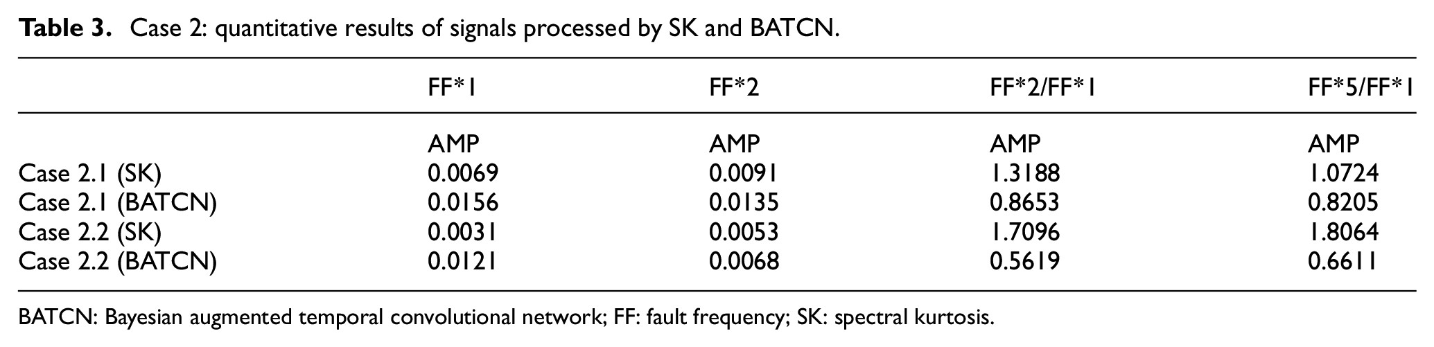
BATCN: Bayesian augmented temporal convolutional network; FF: fault frequency; SK: spectral kurtosis.
In addition, Figure 17 presents the visible intermediate processing results of the SK method, which could explain why the SK method perform less satisfactory in this case. As can be seen in Figure 17(a) and (c), the best window size 768 and 1024 are determined by fast kurtogram algorithm, respectively; subsequently, using this window size to calculate corresponding SK Figure 17(b) and (d). We can observe that SK is uniformly distributed, and values around the best centre frequency are not all higher than the other frequencies. This denotes that the SK method may be difficult to distinguish FF from other frequencies.
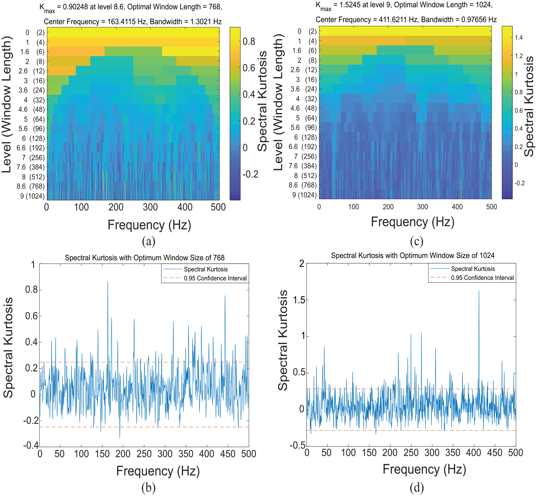
Visible intermediate processing results (a) fast kurtogram results and (b) SK with best window size.
To inspect the inner conditions of pitch bearings of the industrial-scale wind turbine, an electronic endoscope is applied in this case. Figure 18 from endoscope indicates that the defect truly exists at the bearing inner race, measured length 9 mm and width 5 mm. Furthermore, no obvious damage is found in the bearing balls or outer race. This inspection result denotes that the aforementioned diagnostic results are convincing. As a result, the proposed BATCN method in this study might be beneficial for fault diagnosis of wind turbine pitch bearings, demonstrating that this method has a wide range of applications in a natural industrial occasion.
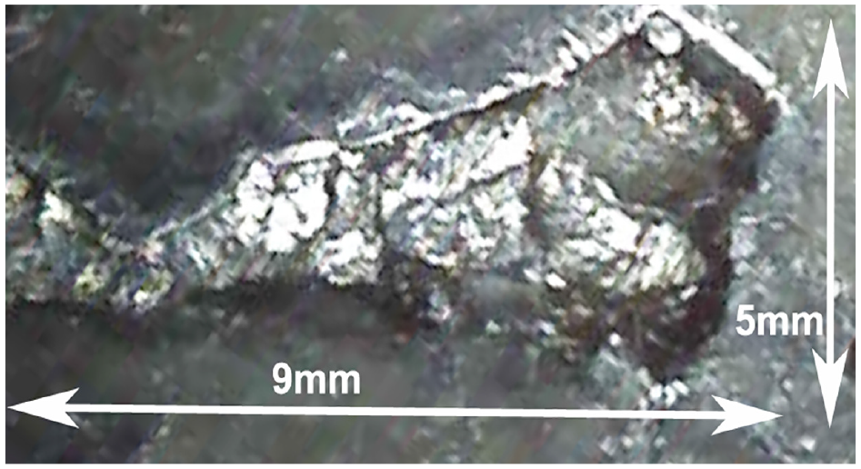
Inner race defect through endoscope.
Case 3
The data in case 3 is also collected with a sampling frequency of 100k Hz and then downsampled to 1k Hz from a real-world wind turbine pitch bearing, which is working in a real-world wind farm but working abnormally. The speed of wind turbine pitch bearing is estimated to range from 1.009 to 1.075 r/min (average speed: 1.042 r/min). Then, substituting into inherent parameters and average speed, the theoretical FFs can be calculated: BPFI 0.535 Hz, BPFO 0.503 Hz and ball spin frequency (BSP) 0.161 Hz.
Figure 19 shows the actual wind turbine pitch bearing in field test. The characteristic of this case is that the data were collected during the operation of the wind turbine, which means that the collected raw data may have a certain degree of disorderliness, as depicted in Figure 20(a). This disorderliness is usually caused by the reciprocating motion of the bearing. 41 To eliminate the influence of reciprocating motion, the collected data are spliced together to obtain an ordered signal, as depicted in Figure 20(b).
The actual wind turbine pitch bearing in field test.
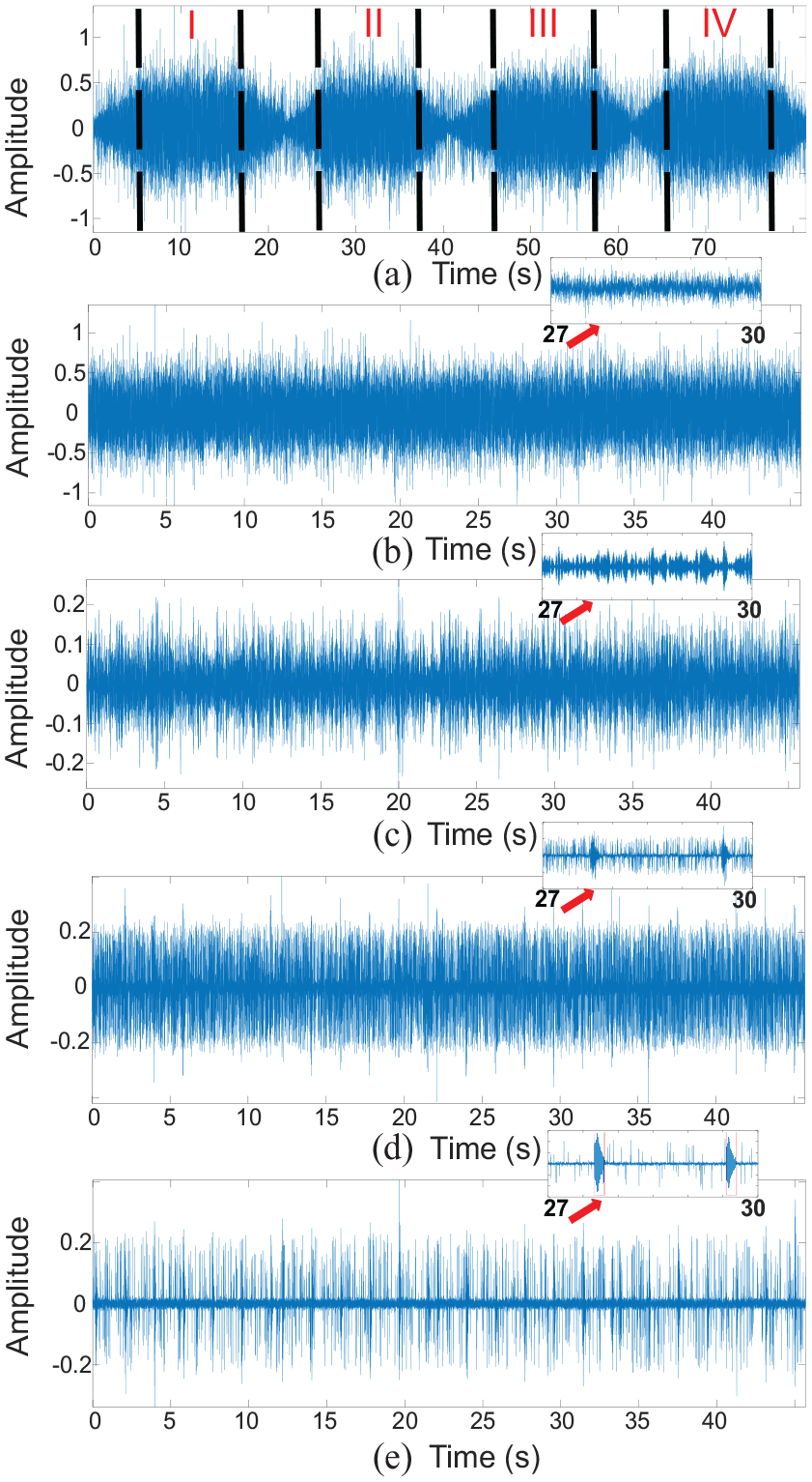
Field wind turbine pitch bearing, case 3 (a) raw signals under the reciprocating operation condition, (b) recombined signals with the four parts in (a), (c) SK denoised signals, (d) TCN denoised signals and (e) BATCN denoised signals.
As shown in Figure 21, the proposed BATCN method can identify FF more clearly than the SK method. It is noted that FF marked in Figure 21(c) is 0.530 Hz. By comparing the theoretical FFs, we can find that FF matches with BPFI, so we can infer that this bearing may exist the inner fault. Similar to the Tables 1 and 3, the Table 4 also demonstrates that the BATCN method is more effective in capturing the FFs in the spectrum.
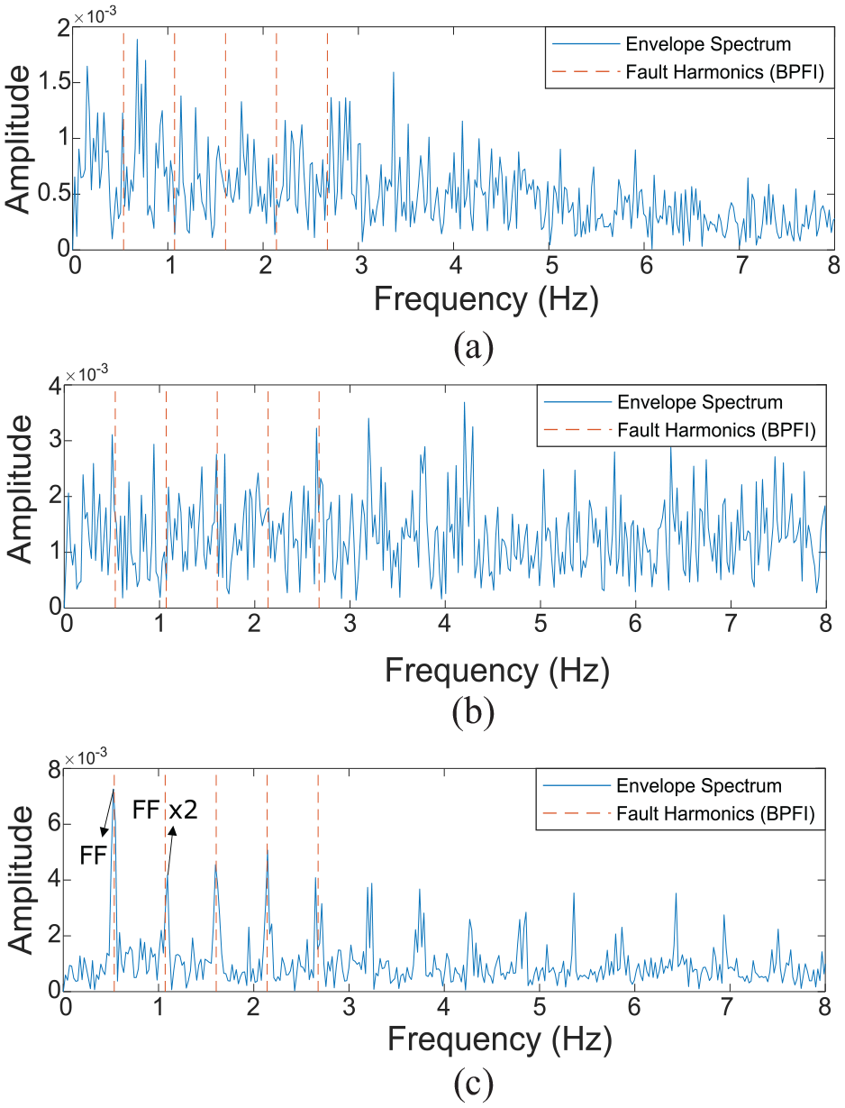
Field wind turbine pitch bearing, case 3 (a) Hilbert envelope spectrum based on SK denoised signals, (b) Hilbert envelope spectrum based on TCN denoised signals and (c) Hilbert envelope spectrum based on BATCN denoised signals.
Case 3: quantitative results of signals processed by SK and BATCN.
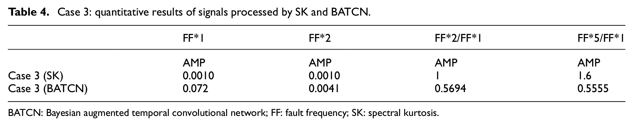
BATCN: Bayesian augmented temporal convolutional network; FF: fault frequency; SK: spectral kurtosis.
Meta-analysis
This section shows a comprehensive analysis on our proposed method. To automatically reflect the damage information from spectra, an indicator

where
Indicator evaluation for cases 1, 2 and 3.
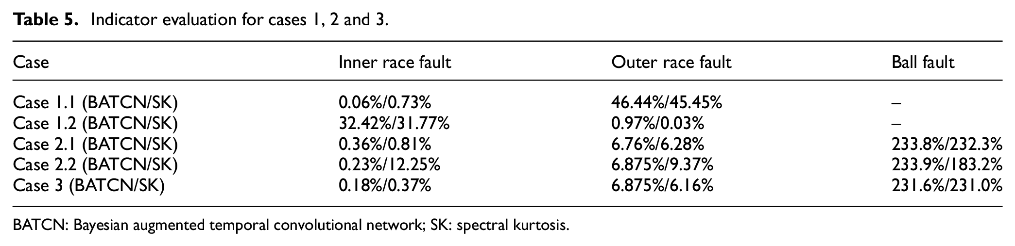
BATCN: Bayesian augmented temporal convolutional network; SK: spectral kurtosis.
To further evaluate our proposed method, we conducted extensive experiments under laboratory conditions to simulate different operating speeds. As shown in Table 6, the bearing defect frequencies were successfully identified using the proposed method, and all of them matched with the theoretical inner race defect frequencies. In addition, the BATCN method is more capable of detecting the correct FF than the SK method, as evidenced by the indicator
Extensive experiments.
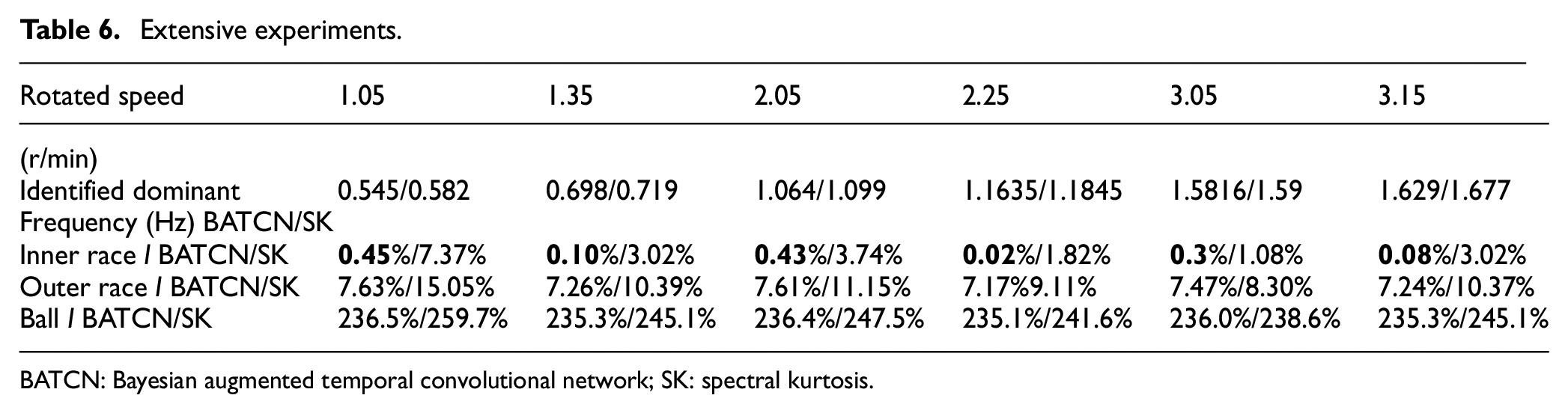
BATCN: Bayesian augmented temporal convolutional network; SK: spectral kurtosis.
In our experiments, the SK method could also detect the FF in some cases, such as results in Figure 14. Unsatisfactory results may be caused by insufficient data length. One characteristic of the SK method is that, as a frequency method, the detection performance improves as the number of repetitions of the fault signal increases. It means that the data length may need to be ensured to obtain multiple repetition of fault signals. This article could demonstrate that the BATCN is capable of working effectively with limited data length, whereas the classical SK method is not.
Conclusion
A signal denoising method, BATCN, is proposed for wind turbine pitch bearing defect detection with slow speed. The BATCN method can learn the intrinsic features of fault signals to guarantee the extraction of non-stationary fault signals and realize noise suppression and harmonic interference suppression during the process of signal denoising, with deep learning techniques. In addition, this new method is able to spontaneously find the best patch length that is a significant performance influence factor under the Bayesian framework. The effectiveness of the new method has been extensively validated on simulation examples and on three real cases (open-source data, lab data and field data). The comprehensive results show the BATCN method is effective in detecting faults for slow-speed wind turbine pitch bearings due to its superior filtering capacity, and it also outperforms the popular SK method.
Footnotes
Declaration of conflicting interests
The authors declared no potential conflicts of interest with respect to the research, authorship, and/or publication of this article.
Funding
The author(s) disclosed receipt of the following financial support for the research, authorship, and/or publication of this article: This work was supported in part by the RCUK under Grant (EP/S017224/1).