Sage Journals: Discover world-class research

Abstract

In this paper, the fatigue state estimation of the metro bogie frame is discussed based on limited sensors through frequency domain methods. The middle-frequency and high-frequency vibration fatigue damage cases of one metro bogie frame is discussed. The main excitations come from the wheel/rail interactions including wheel out-of-roundness and rail irregularities. The most common modal vibration of the bogie frame, where the transom bending deformation is dominant, is taken as the research object to study the possibilities of fatigue failure monitoring on concerned points of the bogie frame transom focusing on specific transfer paths. To eliminate unnecessary input signals which are not closely related to the occurrence of large stress amplitudes, the coherence analysis of different loads including the transmission load, carbody load and wheel-rail impact load is conducted through various methods including the short-time Fourier transform spectrum analysis, the magnitude-squared coherence analysis and the partial directed coherence analysis. Then the power spectral densities (PSDs) of the measured accelerations and cross power spectral densities (CPSDs) are calculated to obtain the transfer functions, whose output is the Y-axis stress at the concerned point. The stress PSDs are obtained using the instantly measured input accelerations and the prepared transfer function. Then the spectral moments and the stress amplitudes distribution functions are calculated through the frequency domain method to overcome the computational burden. The stress reconstructions based on inverse fast Fourier transform are analyzed and the fatigue damage results show good consistency with the experimental ones.

Keywords

State estimation vibration fatigue bogie frame wheel OOR modal vibration coherence analysis transfer function

Introduction

With the rapid development of metro lines in China, operational safety problems have attracted continuous attention. As an important part of the metro vehicle, the bogie frame is subjected to complex loads as well as frequent starting and braking. The excitations mainly come from wheel/rail interactions, which include the wheel out-of-roundness (wheel OOR), wheel flat, rail corrugations, rail welded joints, etc,^1,2 while the others may be related to the traction and braking systems, etc. When the frequency of the external load is close to the modal frequency of the structure, the resonance vibration will arise and cause the fatigue failure problem. Li et al.³ investigated the fatigue failure phenomena of the metro lifeguard, which was caused by the 9th-order wheel OOR. The corresponding resonance frequency of 63 Hz is identical to the bending mode of the lifeguard. Wu et al.⁴ pointed out that the rail corrugation-induced impact with a passing frequency of 78 Hz is the main reason for the modal resonance of the antenna beam in the metro bogie. Wang et al.⁵ found that the 17th-order wheel OOR could motivate the 1st expansion modal of the coil spring in the locomotives. Similar fatigue failure phenomena of the coil spring in metro bogie were reported, which could be explained by P2 force and rail corrugation response.⁶ Fu et al.⁷ found that the wheel-rail impact force P2 accounts for the crack in the bogie beam, which is related to the wheel OOR and rail joints with fish plates. Sun et al.⁸ analyzed the relationship between the bending mode of the bogie frame and the wheel/rail irregularities. The common 5th–9th order wheel OOR is the main cause of the resonance vibration. The rail weld irregularity which is related to the P2 resonance could accelerate the formation of wheel OOR. Wu et al.⁹ built a rigid-flexible coupled dynamics model with the 20th-order wheel OOR to study its effect on the fatigue stress of wheel-mounted gearbox housing of a high-speed train. Zhi et al.¹⁰ comprehensively evaluated the fracture mechanism of a fractured wheelset lifting apparatus and proposed a robust fatigue design optimization process. The fatigue failure problems in railway vehicles are common due to various line conditions and the immediate monitoring of the metro vehicle’s abnormal vibration is necessary.

Based on the abovementioned cases, the structural health monitoring systems in the railway industry have been paid more attention to. The widespread use of onboard sensors and wayside devices is helpful in the damage estimation of the key components and the monitoring of the wheel/rail deterioration. Wu et al.¹¹ built an electromechanical model of a high-speed train transmission system to study the possibilities of using motor current signals instead of vibration signals to identify the wheel flat, wheel OOR and hunting motion. Peng et al.¹² developed a wayside calibration device using the continuous wheel-rail force detection method to detect the wheel OOR and wheel offload. The reliability of the device has been verified in an indoor laboratory. Milković et al.¹³ presented a prototype system for wheel-rail contact forces measurement to monitor curving and derailment safety. Bosso et al.¹⁴ developed a concise algorithm to detect wheel flat defects based on the measurement of axle box accelerations which has been integrated into the onboard system. Wei et al.¹⁵ proposed a track condition monitoring scheme using the acceleration signals from metro bogie and car body. The track alignments are obtained from a mathematical model of vehicle dynamics. Other inertial-based onboard devices for comfort assessment and rail track monitoring are also reported, where both inertial sensors and accelerometers are used.¹⁶ In general, the existing structural health monitoring methods in the railway industry mainly employ acceleration signals, inertia system signals, current signals, and measured strain, etc, where the main index of running comfort and safety are mostly obtained through indirect measurement. The abovementioned abnormal vibration monitoring methods focus on the identification of wheel/rail irregularities or the comfort assessment of the car body. Few studies related to the monitoring of the bogie frame’s resonance vibration and damage estimation have been reported.

To solve the problem, Hong et al.¹⁷ proposed an onboard structural monitoring system using active ultrasonic waves to detect cracks in the bogie frame. Wu et al.¹⁸ developed an online estimation scheme of fatigue damage to the metro antenna beam in a bogie frame using axle box accelerations and stress of the antenna beam. Ugras et al.¹⁹ developed a real-time fatigue damage estimation algorithm for high cycle fatigue of vehicle components using onboard equipment and a single input/single output system was built. Cai et al.²⁰ studied the use of guided waves for the health monitoring and management of bogie frames. The excitation frequency and the suitable mode which is sensitive to cracks are settled by the finite element method. In general, the structural health monitoring of the bogie frame lacks diversified methods and requires further research. Due to the complex external loads, the abnormal vibration monitoring and damage estimation of the bogie frame requires more efficient and simpler ways with less computational burden. For the lack of space and restrictions of experimental conditions, the number of available sensors is relatively small. Normally the dominant mode of the bogie frame which is sensitive to the crack could be settled by experimental results or finite element analysis. Thus the number of employed sensor channels could be reduced due to certain failure modes of the bogie frame. In general, further research on fatigue damage monitoring of metro bogies by using limited sensors is meaningful.

The fatigue damage calculation mainly consists of time domain and frequency domain methods.²¹ In the time domain methods, the dynamic stress could be obtained directly from experimental results or simulations. The stress-time history of critical locations is normally processed by the rain flow counting (RFC) method to obtain the time domain load spectrum. Liu et al.²² used the experimental results and proposed a novel load spectra development method to investigate the fatigue failure problem of the anti-yaw damper seat of railway vehicles. Liu et al.²³ used the measured axle box accelerations as the input to conduct the structural optimization of the bogie frame cowcatchers, which encountered the fatigue failure problem due to modal vibration and rail corrugations. At the same time, Wei et al.^8,24 established a rigid-flexible coupling multi-body dynamics system (MBDS) model to simulate the fatigue failure phenomena of the cowcatcher and analyzed the effect of the rail corrugations. Mei et al.²⁵ proposed a fatigue test load spectrum compilation method for key pantograph components to study the reduction of the pantograph development cycle and optimization of its structural design. In general, the modal vibration has been paid more attention and the rigid-flexible coupling MBDS model of the mechanical system has become more comprehensive. The field tests are focusing on establishing a more suitable load spectrum compilation method according to the actual rail vehicle’s vibration environment in China, where the non-normality and nonstationarity of the signal are very apparent.²⁶

In the frequency domain method, the power spectral densities (PSD) of stress at concerning points is used to predict the probability density distribution function (PDF) of the time domain load spectrum. The well-known frequency domain methods include Dirlik, Zhao-Baker, Tovo-Benasciutti, Gao-Moan methods, etc.²⁷ The method selection and correction are determined by the spectral bandwidth and the PDF of the rain-flow cycling amplitude. One research highlight is the accurate fatigue damage estimation of the non-normal and non-stationary stress in the frequency domain. The related researches are focusing on the transformation of the non-normal signals into normal ones. Wolfsteiner et al.²⁸ proposed a method which is based on a decomposition of non-normal loads in normal portions using the PSD approach. Dou et al.²⁹ introduced the fatigue damage spectrum tool into an approach of deriving the damage equivalent from a set of non-normal accelerations. The existing researches concerning the railway vehicles are focusing on two aspects. One is the accurate estimation of the input excitation like PSDs of the axle box accelerations, which show different characteristics from that in standard EN 61373.^26,30 Another one is the processing procedures of the non-normal stress. But the vibration transmission of the multi input/output system in the frequency domain and the corresponding stress evaluations still need further research. In general, the frequency domain method is more efficient because the time domain approach requires a long computational time when many signals need to be analyzed.

Thus in this study, the in situ experiments of the metro bogie frame are presented, including the fatigue crack analysis and the vibration characteristics test. The coherence analysis in the time domain and frequency domain are conducted to select necessary inputs which contribute most to the fatigue failure of the bogie frame. The non-stationarity and non-normality of the stress time histories at concerning points of the bogie frame are analyzed. The frequency response functions are obtained by using experimental data. The PSDs of the vertical axle box accelerations are used to calculate the dynamic stress in the lateral direction at concerning points of the bogie frame, which could help monitor the resonance vibration and fatigue stress of the bogie frame with limited sensors. The amplitude distributions of Y-axis stress using frequency domain methods are analyzed based on predicted and measured data. The comparisons between the reconstructed stress time histories and measured ones are conducted.

In situ investigation of the bogie frame fracture

Background

In the operation of one metro line in China, the fatigue failure phenomena occurred in the bogie frame of an “H”-type box plate frame structure. To analyze the root cause of the abnormal vibration, the field tests were carried out including the acceleration and dynamic stress measurement as well as the wheel OOR test. As shown in Figure 1, the tested metro line consists of 22 depots and the total mileage is 23.9 km from north to south. The maximum operational speed is 80 km/h. The tested bogie consists of two wheelsets, four axle boxes and one bogie frame. The bogie frame is mounted on the axle boxes through primary suspensions consisting of rubber springs. The car body is mounted on the two bogies by secondary suspensions consisting of air springs. The wheel diameter is 840 mm and the wheelbase is 2200 mm.

Figure 1.

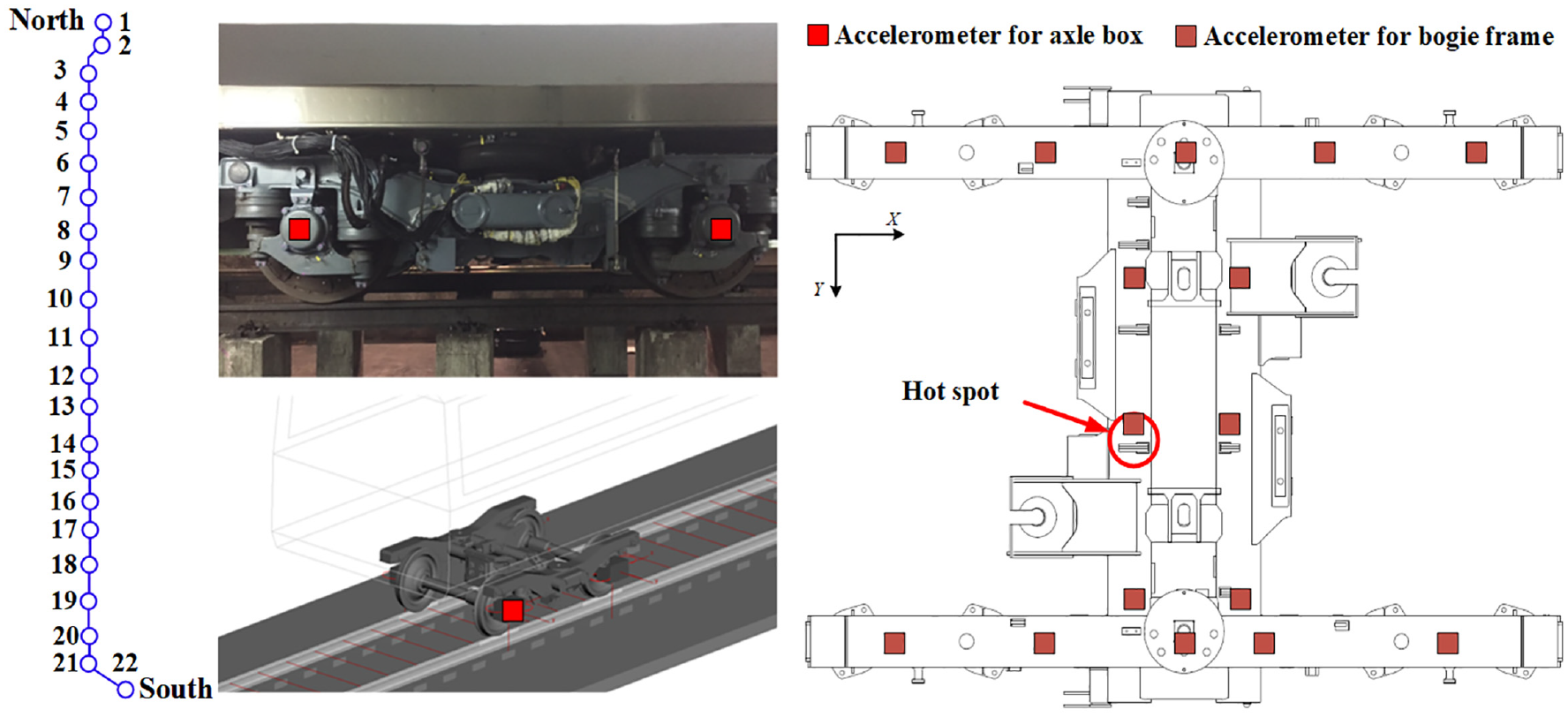
Tested metro line and the accelerometer configuration for the axle box and the bogie frame.

In the test, more than 20 3-axis accelerometers are used to obtain the accelerations of the axle box and bogie frame. And the strain measurement of the hot spot location in the bogie frame is performed to analyze the corresponding dynamic stress characteristics. The sampling rate of the axle box acceleration is 5000 Hz due to high-frequency vibration induced by wheel/rail irregularities. The sampling rate of the bogie frame acceleration and the dynamic stress are 5000 and 2000 Hz respectively. The operational modal deformations of the bogie frame are identified by the PolyMax method³¹ by using the measured accelerations. As shown in Figure 2, the identified modes are as follows: the whole twisting deformation of side beams of 33.4 Hz, the bending deformation of the transoms of 49.5 Hz which is dominant and the pitching deformation of side beams of 56.4 Hz. When the dominant modal vibration of the bogie frame’s transom bending is excited, the dynamic stress in the lateral direction (Y-direction) presents the same frequency of 50 Hz nearby as that of modal deformation, as shown in Figure 3.

Figure 2.

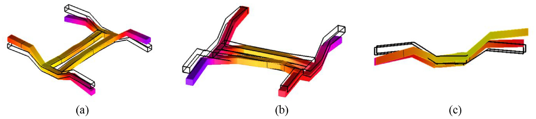
The identified modal deformation in operation: (a) whole twisting deformation of side beams (31 Hz), (b) bending of transoms (50.5 Hz), and (c) pitching mode (56.4 Hz).

Figure 3.

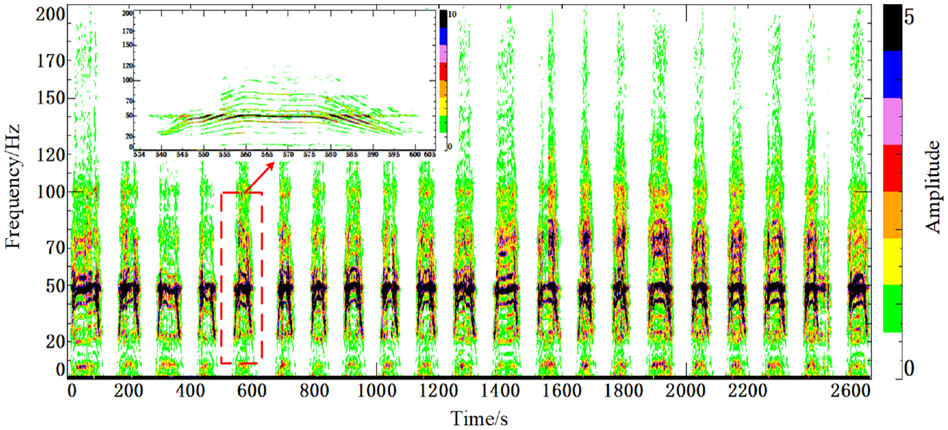
The time–frequency relationship diagram: the hot spot stress in the lateral direction.

The wheel OOR measurement instrument and the measured wheel OOR irregularities are shown in Figure 4. It reveals that the 5th–9th order wheel OOR is the main cause of the input excitation for the bogie frame. The excitation frequencies of the axle box accelerations range from 40 to 70 Hz with a running speed of 60–80 km/h.

Figure 4.

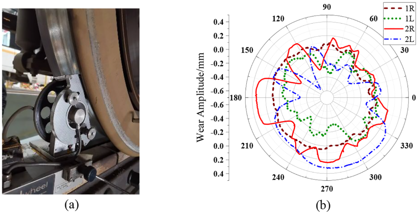
The field test of the wheel OOR: (a) the test equipment and (b) the wheel OOR results of four wheels.

Motivation

Due to the harsh operational environment, the vehicle bogie is subjected to complex excitations caused by external and internal factors, including irregularities from wheel/rail interactions, modal vibration of the bogie frame, voltage pulsation of transmission systems,³² and so on. Thus the general maintenance of the sensors mounted on the bogie is a challenge. Besides, the limited installation space of sensors and data channels, as well as the lightweight requirement for energy saving also need a set of simplified structural safety monitoring methods using fewer sensors.

In this study, a specific and common pattern of abnormal vibration in the metro bogie is used as a research subject. The point of this vibration pattern is the bending deformation of the transom, which has already become one of the most common and harmful factors for the metro bogie frame’s structural safety. Similar cases of fatigue failure phenomena have been reported.^7,8 In these cases, the cracks are normally located at the transom or motor hangers nearby due to the bogie frame’s first bending deformation as shown in Figure 2(b) and the transom bending deformation due to the motors’ vertical vibration. Thus the crack propagation direction is vertical (in the z-axis as shown in Figure 1). Then the Y-axis stress is used as the evaluation index, the direction of which is vertical to the crack propagation direction.

In this section, the influences of different loads are discussed from characteristics in both the time domain and frequency domain, including the acceleration amplitudes, the short-time Fourier transform (STFT) spectrum, the magnitude-squared coherence (MSC) analysis, and the partial directed coherence (PDC) analysis. A brief introduction of the coherence analysis is provided below and for detailed information please refer to pieces of literature.^33,34 In this study, the MSC method is used to find the correlations between the input signals and the output in the specific frequency band. The MSC is a function of the power spectral densities (PSD) that assesses the strength of association and relative linearity between two time series on a scale from 0 to 1.³⁵ The formula of the MSC method is shown as follows:

C_{xy} (f) = \frac{{| P_{xy} (f) |}^{2}}{P_{xx} (f) P_{yy} (f)}

(1)

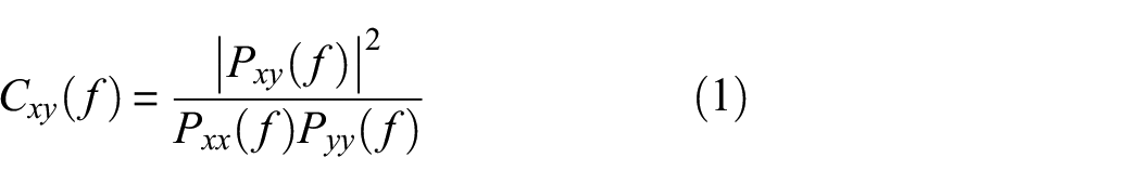
where P_xx (f) and P_yy (f) are the PSD of x and y respectively. And P_xy (f) is the cross power spectral density (CPSD) of x and y. The Welch’s overlapped averaged periodogram method³⁶ was used here and the Hamming window was used to divide the signal into segments with a 50% overlap on each segment.

But the erroneous high coherence may exist due to the high coherence between the inputs. As shown in Figure 5, when a high coherence exists between X1 and X2, one would assume that a physical linear system exists relating these two variables as input and output. But assume that there is a third variable X3, which is also highly coherent with X1, then the high coherence between X1 and X2 might be just a reflection of the fact that X1 is highly coherent with X3 which is related to X2 via a linear system.³⁷ The direct connection between two channels could be confounded by shared inputs from the third channel and the partial coherence method will handle the pairs of interest of the channels in the system and “filter” the shared input.³⁸

Figure 5.

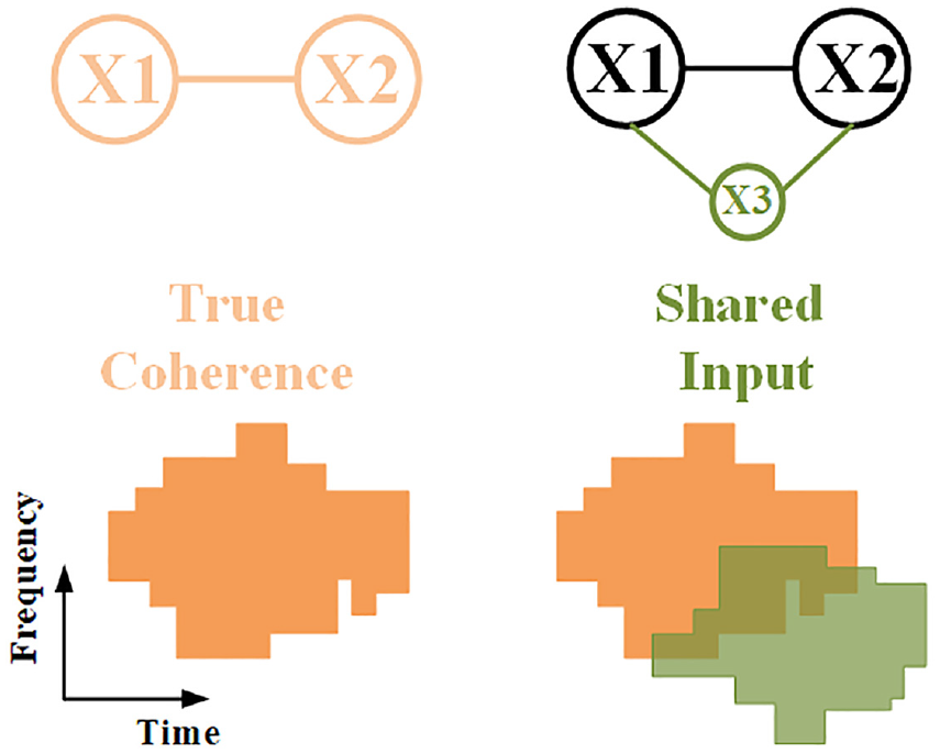
The diagram of erroneous high coherence.

Thus to avoid false positive values, the PDC method is adopted,^39,40 which is a multivariate time-series technique obtained from the factorization of partial coherence and is widely used for evaluating the connectivity between neural structures. This method assumes that the multivariate time series data x(n) could be represented by the pth vector autoregressive model as follows:

x (n) = \sum_{r = 1}^{p} A_{r} x (n - r) + w (n), r > 0

(2)

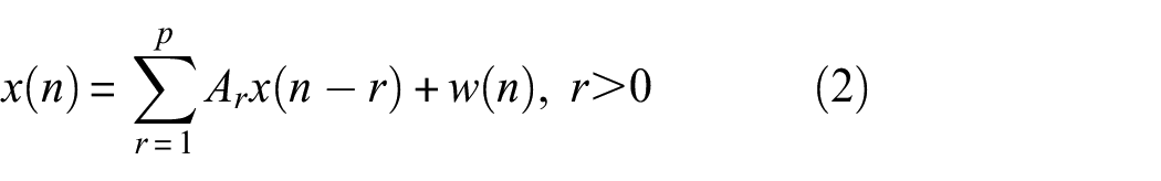
where A_r is the coefficients matrix that describes the linear relationships between time series; w(n) denotes zero mean white processes and its covariance matrix is represented by Σ_w. The joint spectral matrix of x(n) could be expressed as:

S (v) = H (v) \sum_{w} H^{H} (v)

(3)

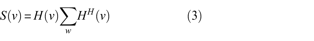
where H^H is the Hermite transpose matrix and

H (v) = {\bar{A}}^{- 1} (v)

(4)

{\bar{A}}_{ij} (v) = {\begin{matrix} 1 - \sum_{r} a_{ij} (r) e^{- j 2 π vr}, & if i = j \\ - \sum_{r} a_{ij} (r) e^{- j 2 π vr}, & if i \neq j \end{matrix}

(5)

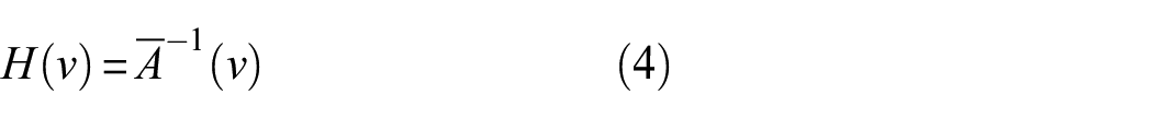
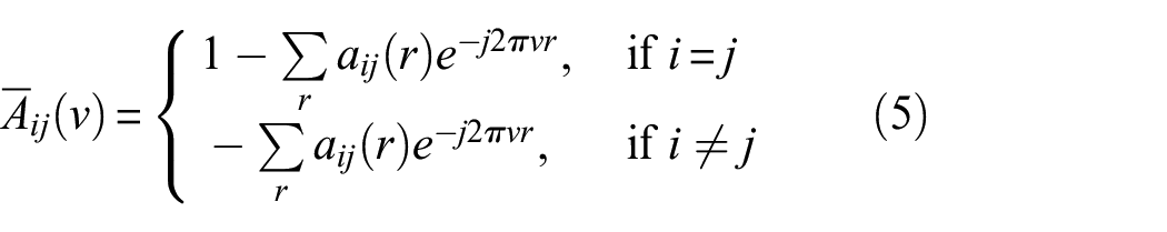
Then Equation (3) could be expressed as:

S_{ij} (v) = h_{i} (v) \sum_{w} h_{j}^{H} (v)

(6)

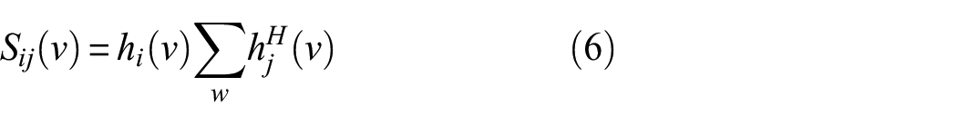
And the coherence between x_i (n) and x_j (n) is:

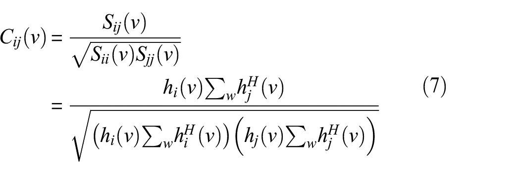
\begin{matrix} C_{ij} (v) = \frac{S_{ij} (v)}{\sqrt{S_{ii} (v) S_{jj} (v)}} \\ = \frac{h_{i} (v) \sum_{w} h_{j}^{H} (v)}{\sqrt{(h_{i} (v) \sum_{w} h_{i}^{H} (v)) (h_{j} (v) \sum_{w} h_{j}^{H} (v))}} \end{matrix}

(7)

The correlation results represent the relevance level between different channels within the selected frequency band. The closer the value is to 1, the higher the relevance level.

In general, the first bending mode of the bogie frame’s transom is easily excited in operation, the corresponding stress direction of which points to the Y-axis, as shown in Figure 9. Besides the bending mode of the bogie frame has led to a series of fatigue failure problems. So the only stress in Y-axis is calculated to exclude the effects of unnecessary stress components and save computing resources. The abovementioned conclusions are also based on the engineering application experience in the past ten years by different researchers.^7,24

Based on the abovementioned methods, the influences of different loads were analyzed and the main loads contributing most to the Y-direction stress at the concerning point were selected for condition-based structural health monitoring of the bogie frame.

Analysis of different loads’ influences on the stress state of the bogie frame

In this section, the loads which are applied at the bogie frame were analyzed. As shown in Figure 6(a), the bogie frame is mainly subjected to vertical loads from the car body through secondary suspension, wheel/rail interactions through primary suspensions as well as transmission load during the starting and braking conditions.

Figure 6.

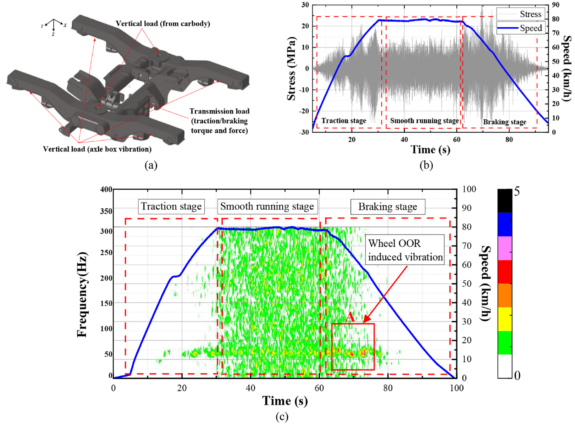
(a) Structure and force description of bogie frame, (b) time history, and (c) time–frequency relationship diagram of traction motor hanger’s vertical acceleration.

As for the transmission load, the traction and brake forces are significant in the vehicle system. According to field test results, the larger stress amplitudes appear during the traction/braking stage, as shown in Figure 6(b). But the abnormal increase of the stress amplitudes arises from the effect of higher orders of wheel OOR at lower speed instead of influences of traction and brake forces. As shown in Figure 6(c), the frequency characteristics of vertical acceleration at the traction motor are not related to speed variation. During the traction stage, the vibration response is very small and doesn’t change with the increase of speed. During the idle running and braking stage, it has similar characteristics. This means the abnormal magnification of stress at the fracture site is not due to traction and brake forces since the vibration characteristics shown in Figure 6(c) lack evidence of influences from motor torque which is related to speed variation. And it’s worth mentioning that in region A as shown in Figure 6(c), some large vibration points near 50 Hz are marked. These points arise from the influence of the bogie frame’s modal resonance vibration (transom bending) with different speeds, which corresponds to different wheel OOR orders and means that the maximum stress amplitudes may occur when vehicles are running at near about 60 km/h.

The axle box acceleration is the direct reflection of the excitations from wheel/rail interactions, which is also the main cause of the bogie frame’s abnormal vibration. As shown in Figure 7(a), the MSC results between axle box lateral acceleration of the front wheel and the Y-axis stress are less than 0.1 and the corresponding results of the rear wheel at 50 Hz reached 0.35, which proves that the Y-axis stress is scarcely influenced by the axle box lateral acceleration. Thus the axle box lateral accelerations were neglected in the following analysis. As shown in Figure 7(b), at the frequency of 50 Hz, the axle box vertical acceleration of the front wheel is less coherent with the Y-axis stress (MSC = 0.6) and the axle box acceleration of the rear wheel is highly related to the Y-axis stress (MSC = 0.9). The differences could be attributed to the following reasons: firstly, the front and rear wheel OOR reached 0.4 and 0.8 mm respectively. Thus the vibration of the rear wheel is more severe; secondly, the concerning point of hotspot stress is close to the rear wheels.

Figure 7.

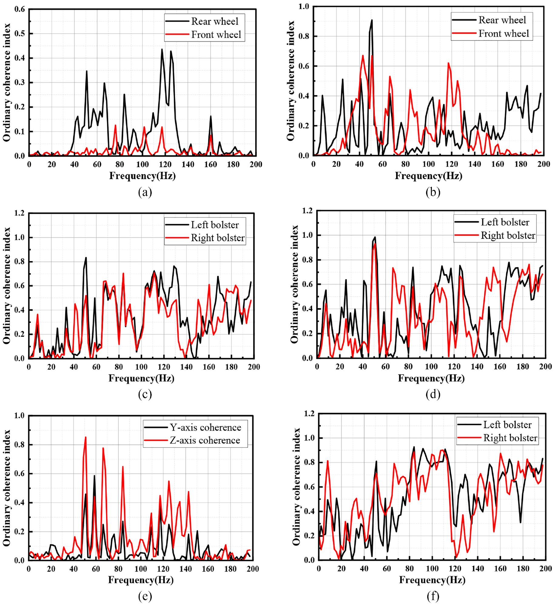
The ordinary coherence index between (a) lateral axle box accelerations and hotspot stress in the lateral direction, (b) vertical axle box accelerations and hotspot stress in the lateral direction, (c) lateral car body bolster accelerations and hotspot stress in the lateral direction, (d) vertical car body bolster accelerations and hotspot stress in the lateral direction, (e) car body bolster accelerations and axle box accelerations in the lateral and vertical direction, and (f) vertical and lateral car body bolster accelerations.

The car body is seated on two bogies by the car body bolsters through four air springs as shown in Figure 6(a). Normally the vibration from wheel/rail interactions is transferred from the bogie to the car body through secondary suspensions and the frequency of the car body vertical vibration is mainly below 20 Hz. As shown in Figure 8(a), the vertical acceleration amplitude of the car body bolster is less than 1 g while that of the axle box could reach 10 or 100 g. As shown in Figure 8(b), the STFT result shows that there is no evident vibration in the frequency range below 100 Hz. So the car body’s influence on the bogie frame could be neglected. But the MSC analysis revealed that the car body accelerations in both the vertical and lateral directions are closely related to the lateral stress at the concerning point of the bogie frame. As shown in Figure 7(c), the MSC results at 50 Hz between the lateral car body bolster accelerations and the Y-axis stress could reach 0.8. And the MSC results at 50 Hz between the vertical car body bolster accelerations and the Y-axis stress could reach nearly unity, as shown in Figure 7(d). The abovementioned results could be erroneous positive values as described in Section “Motivation”. The car body bolster vertical acceleration is highly coherent with the axle box vertical acceleration as shown in Figure 7(e). The car body bolster lateral acceleration is partially related to the axle box lateral acceleration as shown in Figure 7(e) (MSC = 0.45) and is highly coherent with the car body bolster vertical acceleration at 50 Hz as shown in Figure 7(f).

Figure 8.

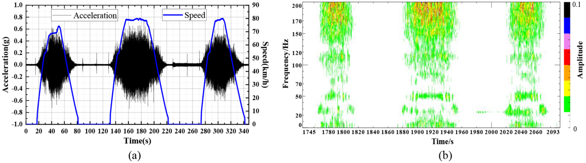
Vertical acceleration of the bolster in car body: (a) time history and (b) the short-time Fourier transform spectra.

To eliminate the influences of shared inputs on the coherence analysis, the PDC analysis was conducted. As shown in Table 1, the Ch1–Ch4 represent the vertical acceleration signals of the four axle boxes. Ch5 and Ch6 represent the lateral and vertical acceleration signals of the left car body bolster respectively, while Ch7 and Ch8 are the corresponding signals from the right car body bolster. Ch9 represents the Y-axis stress of the concerned point in the bogie frame. The PDC results in the last row present the influence of input excitations (Ch1–Ch8) on the output stress (Ch9). The results show that the PDC values between the car body bolster accelerations in both lateral and vertical directions and the Y-axis stress are within 1e-15, which means the car body bolster acceleration will not influence the hotspot stress of the bogie frame in this case.

Table 1.

PDC values between multiple inputs of vibration accelerations and the single output of stress.

p-Values	Ch1	Ch2	Ch3	Ch4	Ch5	Ch6	Ch7	Ch8	Ch9
Ch1		1	1	1	0.0001	8.53e-06	0.0027	3.93e-06	0.00053
Ch2	1		1	1	9.32e-15	0.007	0.0003	0.008	4.29e-08
Ch3	1	1		1	<1e-15	2.36e-05	<1e-15	3.72e-05	<1e-15
Ch4	1	1	1		<1e-15	0.0015	<1e-15	2.25e-06	<1e-15
Ch5	1	1	1	1		<1e-15	<1e-15	<1e-15	<1e-15
Ch6	1	1	1	1	<1e-15		<1e-15	<1e-15	<1e-15
Ch7	1	1	1	1	<1e-15	<1e-15		<1e-15	<1e-15
Ch8	1	1	1	1	<1e-15	<1e-15	<1e-15		<1e-15
Ch9	1	1	1	1	<1e-15	<1e-15	<1e-15	<1e-15

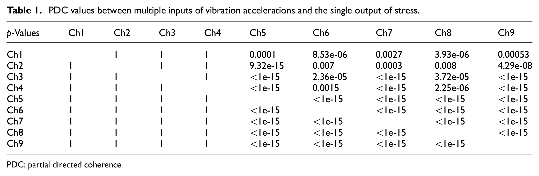
PDC: partial directed coherence.

Methodologies

In this study, the framework for loads analysis and state estimation of one common type of abnormal vibration of the bogie frame is proposed, as shown in Figure 9. The main procedures consist of four parts: firstly, the in situ investigations of the bogie system are conducted to obtain necessary acceleration signals and dynamic hotspot stress; secondly, as described in Section “Analysis of different loads’ influences on the stress state of the bogie frame”, the correlations between different loads and stress of target location are analyzed to get rid of unnecessary inputs by using MSC and PDC analysis; thirdly, the dynamic stress spectrum in the frequency domain are obtained by the product of input excitations in the frequency domain and transfer functions. The transfer functions could be obtained through in situ experiments or numerical models. The last step consists of different fatigue damage estimation methods in the frequency domain and the estimated stress reconstruction. The first two steps have already been introduced in previous sections. The following contents will introduce the detailed procedures of the last two steps.

Figure 9.

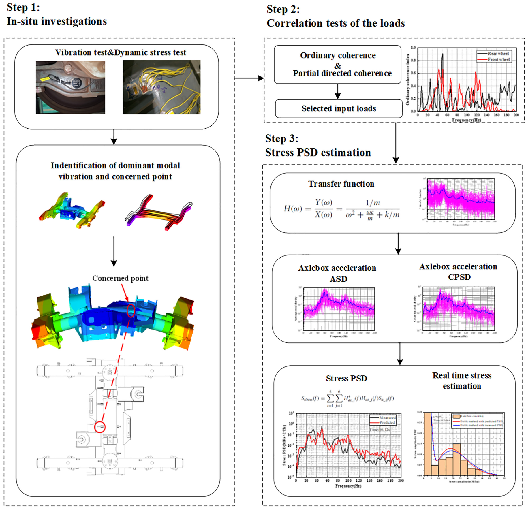
The illustration of the research progress of this paper.

Acquisition of transfer functions and estimation of the dynamic stress spectrum

For the system with a single degree of freedom, consider a stationary random vibration x(t) applied to a linear mechanical system and its response y(t). Their Fourier transforms are linked by:

Y (jw) = H (jw) X (jw)

(8)

where H(jω)is the transfer function matrix. Then we square each member of this equation and according to the auto spectrum definition^38,41:

Y^{*} (jw) Y (jw) = H^{*} (jw) H (jw) X^{*} (jw) X (jw)

(9)

G_{y} (f) = {| H (f) |}^{2} G_{x} (f)

(10)

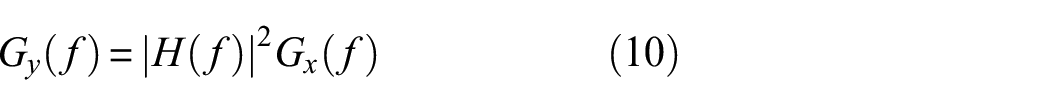
where G_x (f) and G_y (f) are the power spectral densities of the input and output response, respectively.

For a single input/single output (SISO) system, the estimation of the transfer function is given as:

H (f) = \frac{G_{yx} (f)}{G_{xx} (f)}

(11)

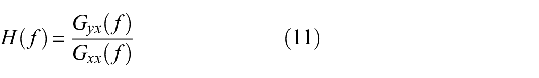
where G_yx (f) is the CPSD of x and y, and G_xx (f) is the PSD of x. For the multi-input/multi-output systems, it has the same mathematical form as the SISO system, where G_yx (f) and G_xx (f) denote the CPSD matrix and PSD matrix of multiple inputs and outputs, respectively.

Then consider the multi-input system, the expression of the output response $G_{y} (f)$ is given as^18,42:

G_{y} (f) = \sum_{r = 1}^{N} \sum_{s = 1}^{N} H_{r}^{*} (f) H_{s} (f) G_{x_{r} - x_{s}} (f)

(12)

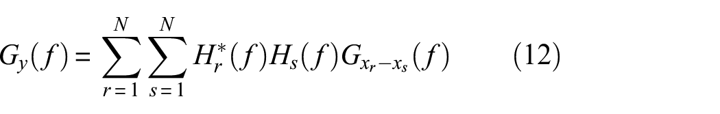
where H* (f) denotes the complex conjugate of transfer function H(f). $G_{x_{r} - x_{s}} (f)$ is the CPSD between the rth and sth input when r ≠ j; when r = j, $G_{x_{r} - x_{s}} (f)$ equals $G_{x} (f)$ which represents the auto-spectral density (ASD) of rth and sth input. In this study, the vertical accelerations of the axle box are used as the input excitation, which could be obtained continuously by onboard devices. Then the PSD of the hotspot stress which served as the output of the system could be calculated through the transfer function and real-time axle box accelerations.

After obtaining the concerned stress PSD, the stress time history could then be reconstructed using the inverse fast Fourier transform (IFFT). Due to the absence of phase information in stress PSD, the reconstruction of stress time histories is based on the uniformly distributed random phases at different frequencies. Due to the phase randomness, the reconstructed time series will be the normal quasi-random ones.⁴³ But the dynamic stress of the bogie frame in this study presents to be the non-normal one in a relatively larger time span of tens of seconds. The underestimation of the stress kurtosis will lead to a lower estimation of the structural damage.²⁷ In the following parts of this study, the time-varying kurtosis in a small time span will be displayed to show the differences with the measured results. And the root mean square (RMS) values could be obtained from both the time histories and frequency domain to validate the proposed method.

The fatigue stress estimation using the frequency domain method

In the frequency domain method, the autocorrelation function and PSD function are used to describe the characteristics of stationary random process in the time domain and frequency domain respectively. According to the Wiener-Sinchin theorem, the autocorrelation function and PSD function form the Fourier transform pair as follows:

S_{x} (ω) = \int_{- \infty}^{\infty} R_{x} (τ) e^{- j ω τ} d τ

(13)

R_{x} (τ) = \frac{1}{2 π} \int_{- \infty}^{\infty} S_{x} (ω) e^{- j ω τ} d ω

(14)

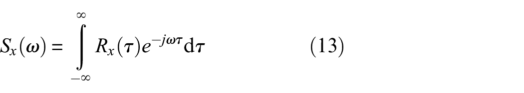
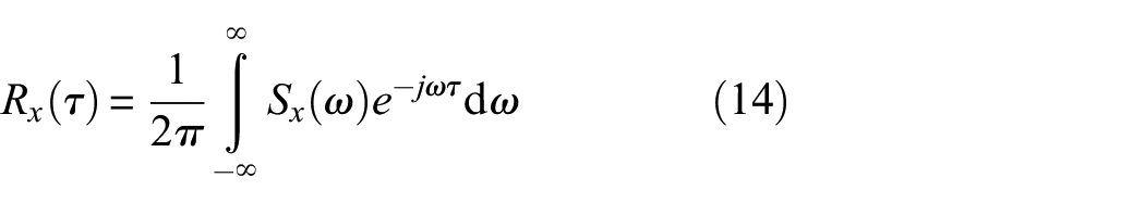
The one-sided PSD function G(ω), where ω varies only over $(0, \infty)$ , is defined by

G (ω) = {\begin{matrix} 2 S_{x} (ω), ω > 0 \\ S_{x} (0), ω = 0 \end{matrix}

(15)

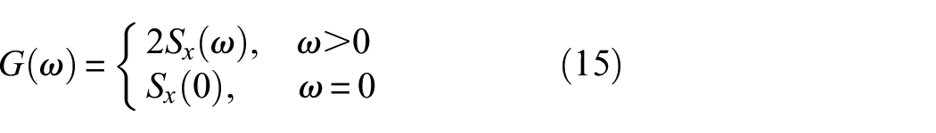
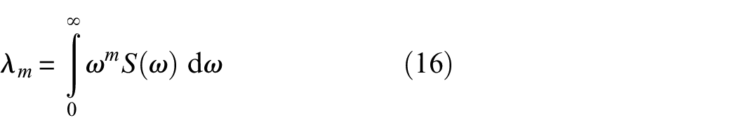
The characteristics of G(ω) can be described by the spectral moment and the spectral width. These two parameters are used for validation of the proposed procedures. Similar to the definition of the statistical moments, the set of spectral moments which is used to describe statistical properties is given:

λ_{m} = \int_{0}^{\infty} ω^{m} S (ω) d ω

(16)

And the bandwidth parameter or the irregularity index r⁴⁴:

r = \frac{λ_{2}}{\sqrt{λ_{0} λ_{4}}}

(17)

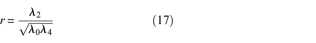
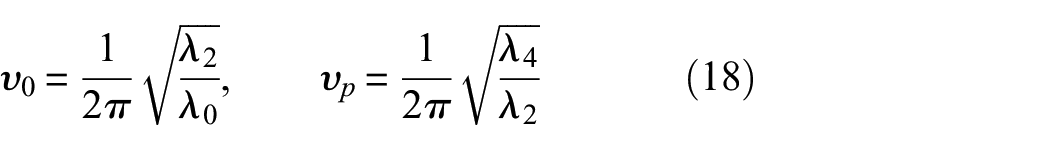
The irregularity index r ranges from 0 to 1. Another form is the Vanmarcke’s spectral parameter $q = \sqrt{1 - r^{2}}$ . If x(t) is narrow-band, r approaches unity, while $x (t)$ is broad-band it converges to zero. The RMS of x(t) is $σ_{x} = \sqrt{λ_{0}}$ . The mean upcrossing rate $υ_{0}$ and its frequency of peaks $υ_{p}$ are, respectively:

υ_{0} = \frac{1}{2 π} \sqrt{\frac{λ_{2}}{λ_{0}}}, υ_{p} = \frac{1}{2 π} \sqrt{\frac{λ_{4}}{λ_{2}}}

(18)

An empirical close-form expression for the probability density function of the rain-flow stress amplitudes was proposed by Dirlik, which was designed to estimate the stress amplitude distribution obtained by the RFC method.⁴⁴ The probability density function of the rain-flow stress amplitudes S is calculated as follows⁴⁴:

p (S) = λ_{0}^{- 1 / 2} \cdot [\frac{D_{1}}{Q} \cdot e^{- \frac{Z}{Q}} + \frac{D_{2} \cdot Z}{R^{2}} \cdot e^{- \frac{Z^{2}}{2 \cdot R^{2}}} + D_{3} \cdot Z \cdot e^{- \frac{Z^{2}}{2}}]

(19)

Z = \frac{S}{\sqrt{λ_{0}}}; χ_{m} = \frac{λ_{1}}{λ_{0}} \cdot \sqrt{\frac{λ_{2}}{λ_{4}}}

(20)

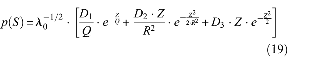
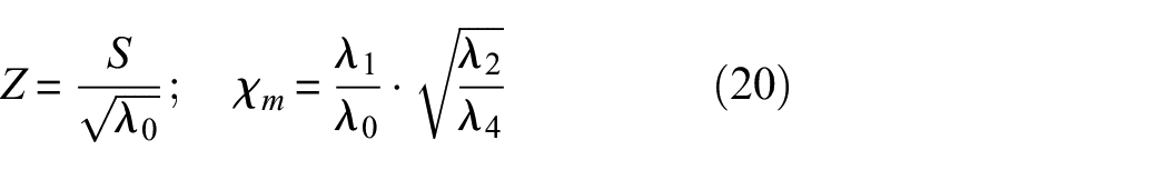
where Z is the normalized stress amplitude and $χ_{m}$ is the mean frequency. And:

\begin{matrix} D_{1} = \frac{2 \cdot (χ_{m} - r^{2})}{1 + r^{2}}; D_{2} = \frac{1 - r - D_{1} + D_{1}^{2}}{1 - R}; \\ D_{3} = 1 - D_{1} - D_{2}; \\ Q = \frac{1.25 \cdot (r - D_{3} - (D_{2} \cdot R))}{D_{1}}; R = \frac{r - χ_{m} - D_{1}^{2}}{1 - r - D_{1} + D_{1}^{2}} . \end{matrix}

(21)

are the spectrum parameters.

The estimated rain-flow damage intensity $\bar{D} (1)$ which denotes the damage per time unit under the Palmgren-Miner rule is calculated as follows⁴⁴:

\bar{D} (1) = υ_{p} \cdot C^{- 1} \cdot \int_{0}^{+ \infty} S^{k} \cdot p (S) \cdot d s

(22)

where C and k represent the fatigue strength and curve slope of the S–N curve.

A case study of the metro bogie frame

As introduced in Section “Motivation”, the bending deformation of bogie frame transom has become one of the most common causes of fatigue failure problems. The concerned point of hot spot stress location is determined based on in situ experiments. Only the vertical axle box accelerations are used as the input excitations of the bogie frame, which are measured in real time through the sensors as shown in Figures 1 and 9. The y-axis stress at the concerned point served as the only output, which is located at the bogie frame transom. Then the whole system could be considered as the four inputs and one output system. As described in Section “Acquisition of transfer functions and estimation of the dynamic stress spectrum”, the stress PSD G_stress (f) could be calculated based on Equation (12)¹⁸:

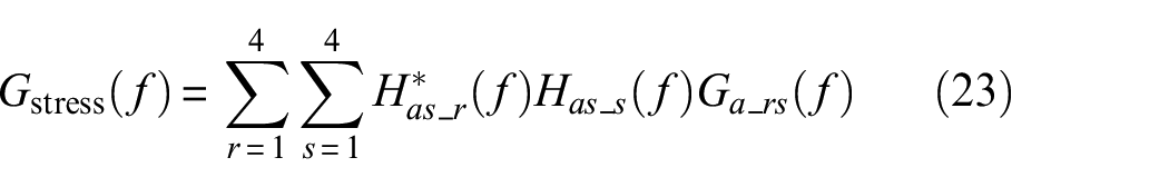
G_{stress} (f) = \sum_{r = 1}^{4} \sum_{s = 1}^{4} H_{as_r}^{*} (f) H_{as_s} (f) G_{a_rs} (f)

(23)

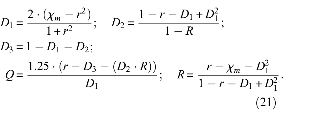
where H_{as_s} (f) is the transfer function between the sth vertical axle box acceleration and dynamic stress of the concerned point. $H_{as_r}^{*} (f)$ is the complex conjugate of the transfer function H_{as_r} (f). G_{a_rs} (f) represents the CPSD of rth- and sth-input accelerations. The estimation method of the transfer function has already been introduced in Section “Acquisition of transfer functions and estimation of the dynamic stress spectrum”, which used the CPSD of each input acceleration to the output stress and the PSD of each input acceleration.

Due to frequent start-ups and brakes during the operation of the metro vehicle, the measured stress and accelerations tend to be non-stationary between the two stations. To quantify the non-stationarity of the signal, the non-stationarity index is used which is defined by the “Run-Test” method.^45,46 In this non-parametric method, the vibration signal is divided by the same window width. Afterward, the change in the variation of the statistical characteristics in relation to the entire signal is analyzed in each window. The run is defined based on the sequence of identical observations which are classified into one of two mutually exclusive designations like greater (+) or less (−) than the RMS value of the entire signal. Assuming that N_i is the number of i observations and N is the total number of windows. Then the mean value $μ_{r}$ and variance $σ_{r}^{2}$ of runs are as follows:

μ_{r} = \frac{2 N_{0} N_{1}}{N} + 1, σ_{r}^{2} = \frac{2 N_{0} N_{1} (2 N_{0} N_{1} - N)}{N^{2} (N - 1)}

(24)

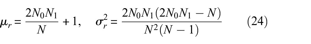
Thus the distribution of the number of runs r is determined by the confidence interval:

μ_{r} \pm α σ_{r}

(25)

where α is equal to 1.96 considering a level of 95% of confidence. If the number of runs falls outside the confidence interval, the signal is considered non-stationary. Hence, the non-stationarity index γ is determined by the number of runs divided by the expected mean number of runs:

γ = \frac{r}{μ_{r}} \times 100 %

(26)

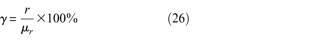
The run-test $V_{n}$ is defined as :

V (n) = {\begin{matrix} 1; & | R_{w} (n) - R_{T} | > σ_{R} \\ 0; & | R_{w} (n) - R_{T} | \leq σ_{R} \end{matrix}

(27)

where R_w (n) is the RMS value of the n-th window, and R_T is the RMS value of the whole signal. σ_R is the standard deviation of all window RMSs.

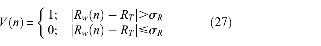
As shown in Figure 10(a), the typical stress time histories are processed for the determination of non-stationarity. The red thick line denotes the standard deviation of each window and the blue dash-dotted lines represent the upper boundary and the lower boundary corresponding to the values of $R_{T} - σ_{R}$ and $R_{T} + σ_{R}$ . The positive or negative signs of the run-test values are determined by whether the standard deviation for each window is located within the boundaries. For example, the non-stationarity index γ equals 0.1933, which is far less than 1 and denotes a nonstationary process. Thus the transfer functions of the vertical axle box accelerations to dynamic stress of the bogie frame are calculated within a shorter time interval, where the measured signals tend to be stationary ones.¹⁸

Figure 10.

(a) The run-test evaluation of Y-axis stress at the concerned point and (b) the irregularity index of the vertical axle box acceleration in different sections.

As shown in Figure 10(b), the irregularity indices of the axle box vertical accelerations in two different sections are mainly within the range from 0.3 to 0.5. It indicates that the axle box vertical accelerations tend to be a broad-band process which could arise from the wheel/rail irregularities including the rail welded joints and rail corrugations as well as different orders and depths of wheel OOR. Due to the resonance vibration of the bogie frame, the dynamic stress tends to be a narrow-band process after the vibration transmission from the axle box to the bogie frame.

Transfer property analysis of the bogie system

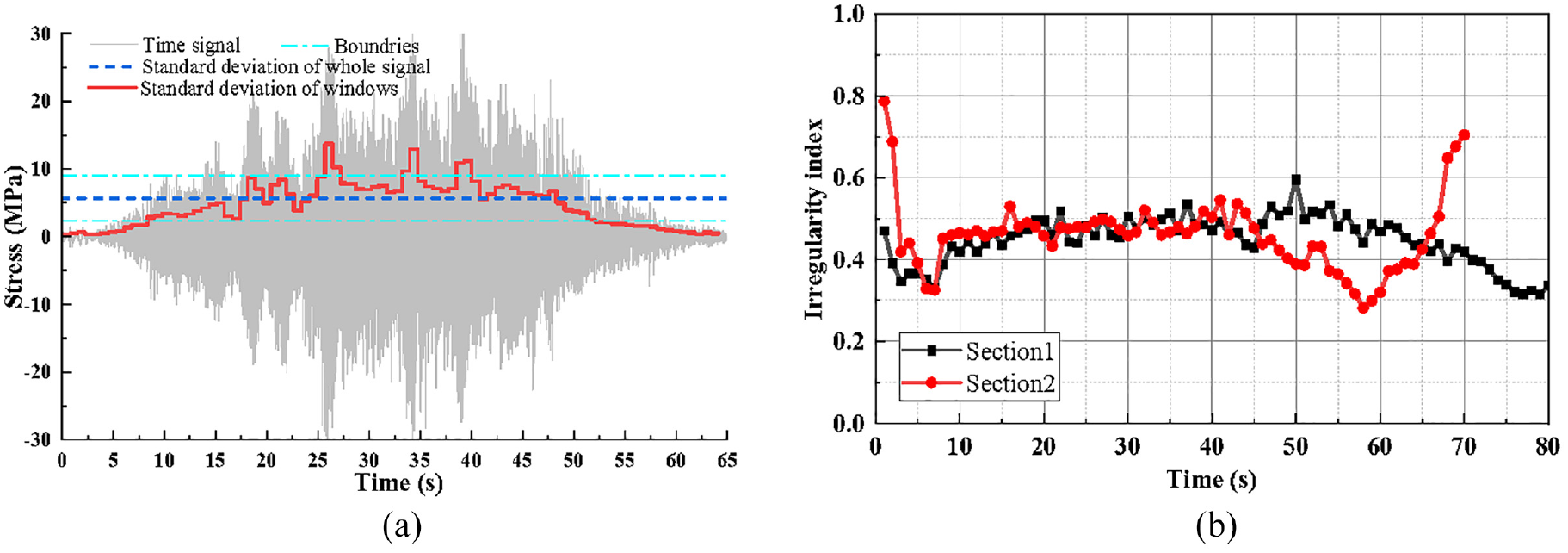
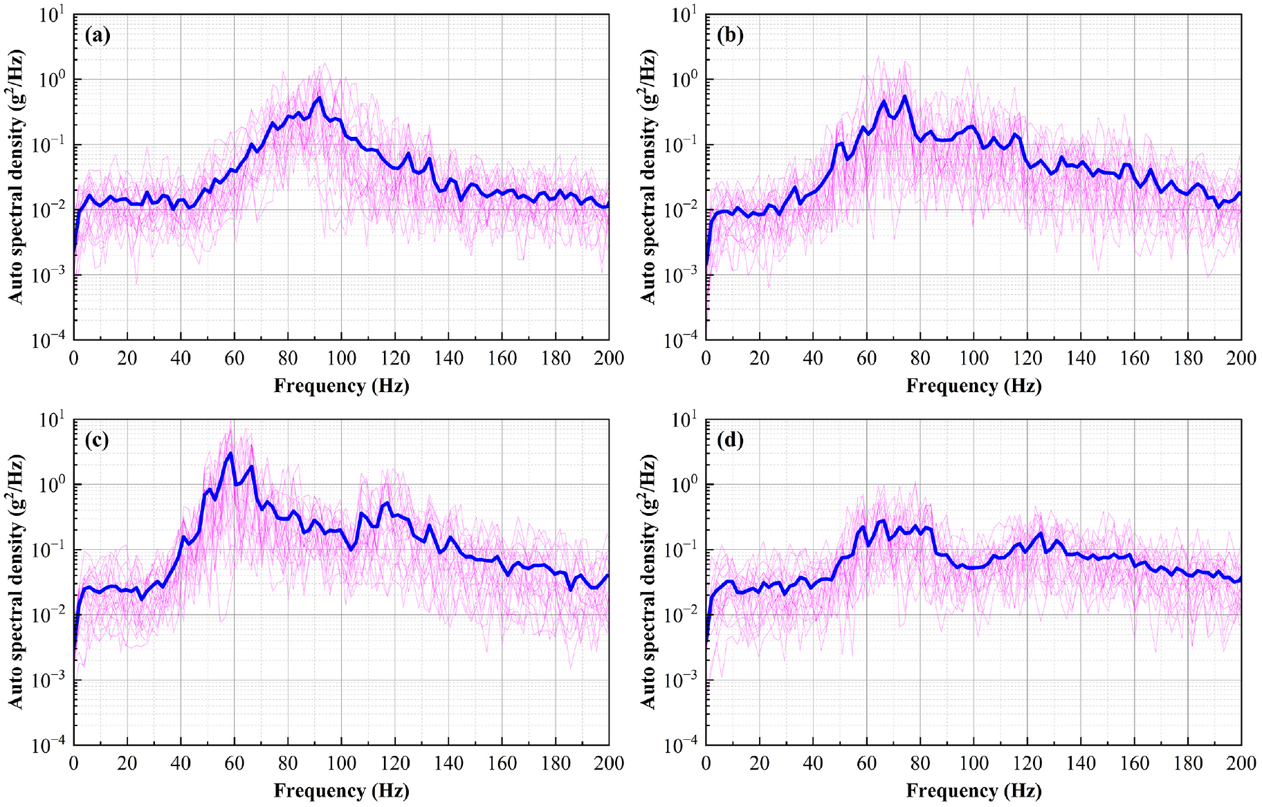
As shown in Figure 11, the ASDs of four vertical axle boxes are illustrated. The dominant frequency band ranges from 40 to 80 Hz. The peak values of ASD amplitudes occurred from 60 to 80 Hz due to various wheel OOR orders. The 5th–9th orders of wheel OOR were found to be dominant. With the running speed from 50 to 80 km/h, the corresponding excitation frequency ranges from 42 to 67 Hz. The OOR of the right wheel is the most severe which reached 0.8 mm and the corresponding peak values of ASD amplitudes are also larger. The CPSDs of axle box vertical accelerations to Y-axis stress at the concerned point are illustrated in Figure 12, which could reflect the correlations between two signals in the frequency domain. It can be seen that the peak values of CPSD amplitudes mainly occurred at 50 and 74 Hz from different axle boxes, which are apparently larger than other frequency bands. It demonstrates that the Y-axis stress is highly correlated with the axle box vertical accelerations in the frequency band of 40 to 74 Hz, especially at the frequency of 50 Hz. This also further proved the correlation between the modal vibration of the bogie frame’s transom bending deformation and the external excitations due to wheel OOR from wheel/rail interactions.

Figure 11.

Auto spectral density of axle boxes: (a), (b) right and left axle box of the front wheel and (c), (d) right and left axle box of the rear wheel.

Figure 12.

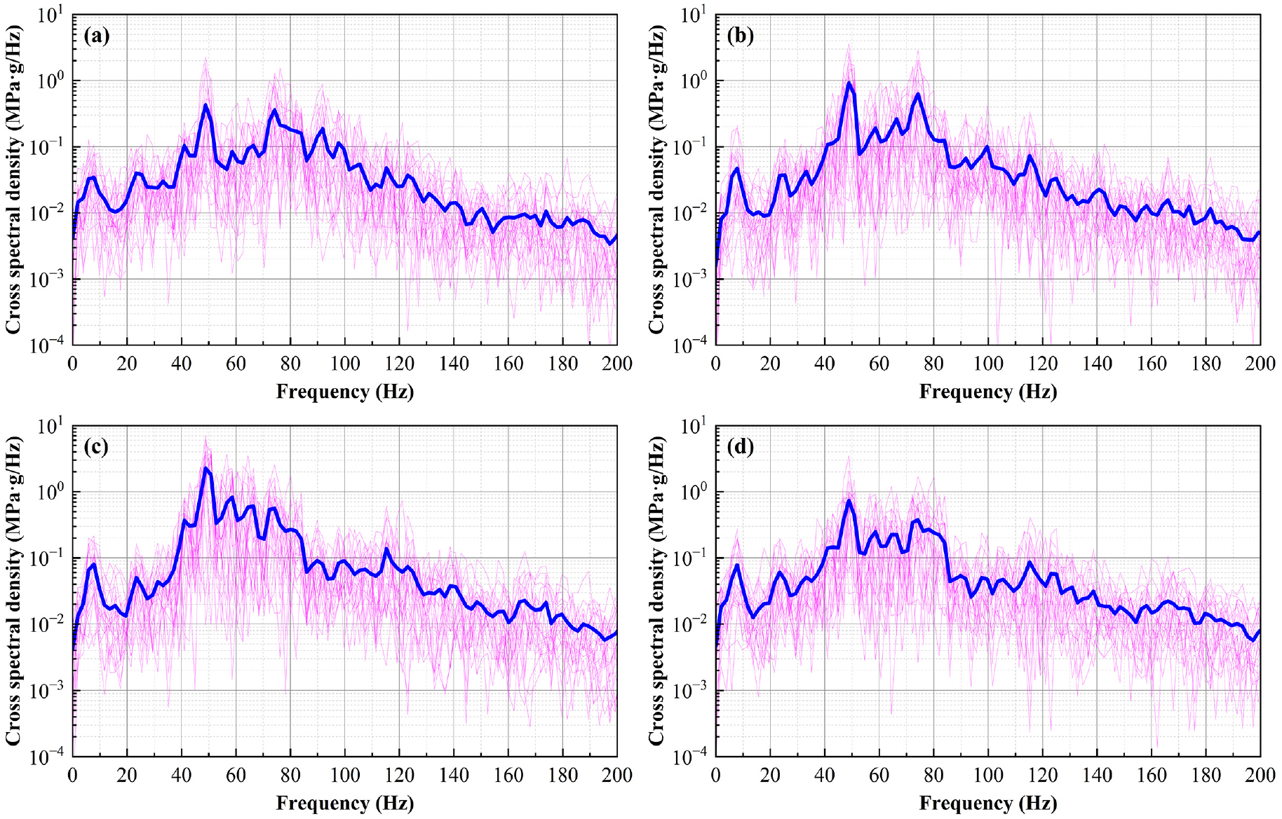
Cross spectral density of axle box accelerations to Y-axis stress at concerned point: (a), (b) right and left axle boxes of the front wheel and (c), (d) right and left axle boxes of the rear wheel.

Then the transfer functions could be calculated in a short time interval using the abovementioned ASDs of the axle box vertical accelerations and the CPSDs of dynamic stress to accelerations. As shown in Figure 13, the transfer functions of each axle box to Y-axis stress are illustrated. The purple solid lines denote the transfer functions calculated from all time intervals and the blue solid lines represent the mean values of these transfer functions. The transfer functions of four inputs to output all demonstrate the high transmissibility from axle box vertical accelerations to dynamic stress near the frequency of 50 Hz. Besides the transmissibility of the frequency band from 30 to 55 Hz and below 10 Hz is obviously larger. According to the experiment results, only the high-frequency components above 20 Hz are obvious, as shown in Figure 3. It can also be seen that the frequency of 8 Hz nearby exists in the whole operation in Figure 3. One may deduce that it could arise from the wheel rotating frequency at running speed of 80 km/h (f = v/2πR = 8.4 Hz). Due to the nonlinearities and the uncertainty of the whole system,¹⁸ the calculated mean transfer functions are used in this study.

Figure 13.

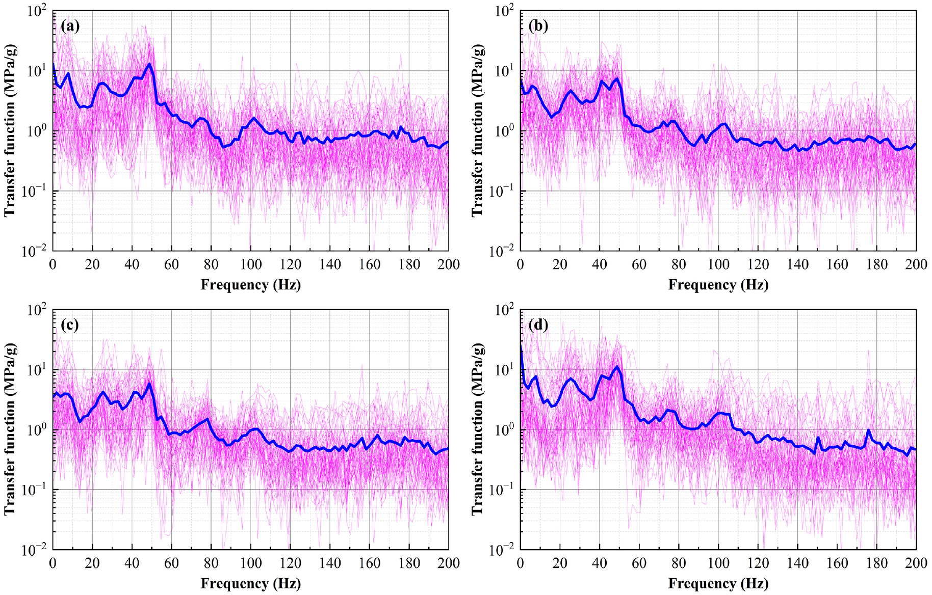
Transfer functions of axle box accelerations to Y-axis stress at concerned point: (a), (b) right and left axle boxes of the front wheel and (c), (d) right and left axle boxes of the rear wheel.

Fatigue stress estimation and damage evaluation

The Y-axis stress PSDs of the bogie frame’s concerned point during each time interval could be calculated based on the obtained transfer function and the PSDs of each axle box vertical acceleration. As shown in Figure 14, the predicted and measured stress PSDs are compared with two selected segments, the time intervals of which are both 2 s, respectively. The peak values of stress PSDs normally occurred at frequencies of nearabout 40 and 50 Hz. It can be seen that the predicted results are quite comparable with the measured results. The predicted results tend to overestimate the amplitudes of PSD results within the frequency band above 100 Hz. Wu et al.¹⁸ deduce that the phenomena could arise from the nonlinearities in the systems. In this case, the nonlinearities could arise from the frequency-varying characteristics of primary suspensions which consist of rubber springs. The RMS values and irregularity indices from both predicted and measured Y-axis stress PSDs are compared to verify the validity of the method, which are described in Section “The fatigue stress estimation using the frequency domain method”. As shown in Figure 15(a) and (b), the RMS values from two sections of 100 and 80 s are plotted and the predicted results show good agreement with the measured ones. As shown in Figure 15(c) and (d), the irregularity indices from the corresponding sections also proved the efficiency of the predicted stress PSDs. The irregularity index describes the shape of the signal’s PSD and the higher value approaching unity denotes a narrow-band process.

Figure 14.

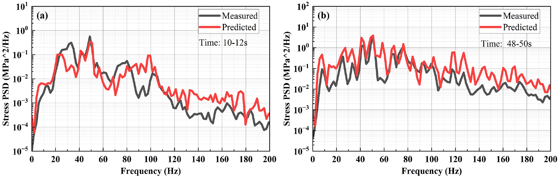
The estimated stress PSDs using the transfer function from section (a) and section (b). .

Figure 15.

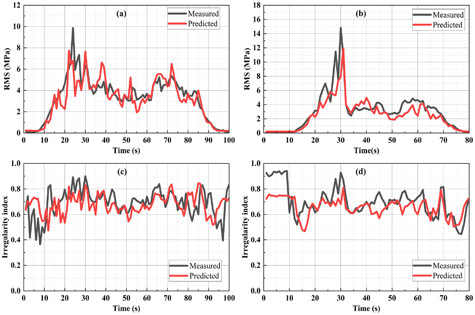
Comparisons of predicted and measured stress PSDs: (a) and (b) RMS values of two selected segments; (c) and (d) the corresponding irregularity indices.

RMS: root mean square.The predicted irregularity indices are mainly in the range of 0.6 to 0.8 while the measured ones vary in the range of 0.7 to 0.9, which could arise from the non-normal characteristics of the process. In general, the proposed method using limited sensors has been proved to be efficient in the prediction of Y-axis stress PSDs in terms of amplitudes of dominant frequencies as well as bandwidth of the PSDs. As shown in Figure 16, the overall errors of RMS values and irregularity index results from the estimated and measured stress PSDs are within 30% and 25% with respect to the measured results, respectively. Besides, the computing efficiency is also important for the real time monitoring. On an average it takes 33–35 s for the whole calculation with the input data of 100 s. Both the stability and the computing efficiency are ensured for the proposed methodology.

Figure 16.

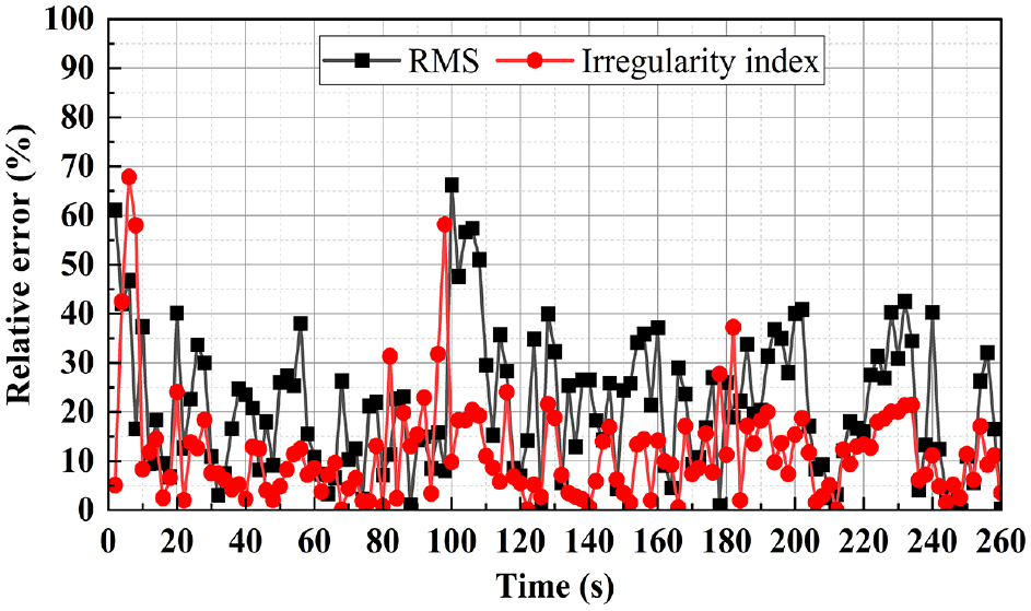
Relative errors of RMS values and irregularity indices between predicted and measured stress results.

Then the PDF estimations of stress amplitudes at concerned points could be calculated in each time interval using the obtained stress PSDs, as introduced in Equation (19). The PDFs of stress amplitudes calculated by the Dirlik method using the measured and predicted PSDs are compared with the RFC results. As shown in Figure 17, three time sections with different irregularity indices are plotted and the PDF estimation results calculated by the Dirlik method are consistent with the RFC results. With the higher irregularity indices of 0.69 which denotes a nearly narrow-band process, the proportion of large stress amplitudes from 10 to 40 MPa increases. With a lower irregularity index of 0.5 nearby, the proportion decreases greatly to nearly zero and the dominant stress amplitudes are within 10 MPa.

Figure 17.

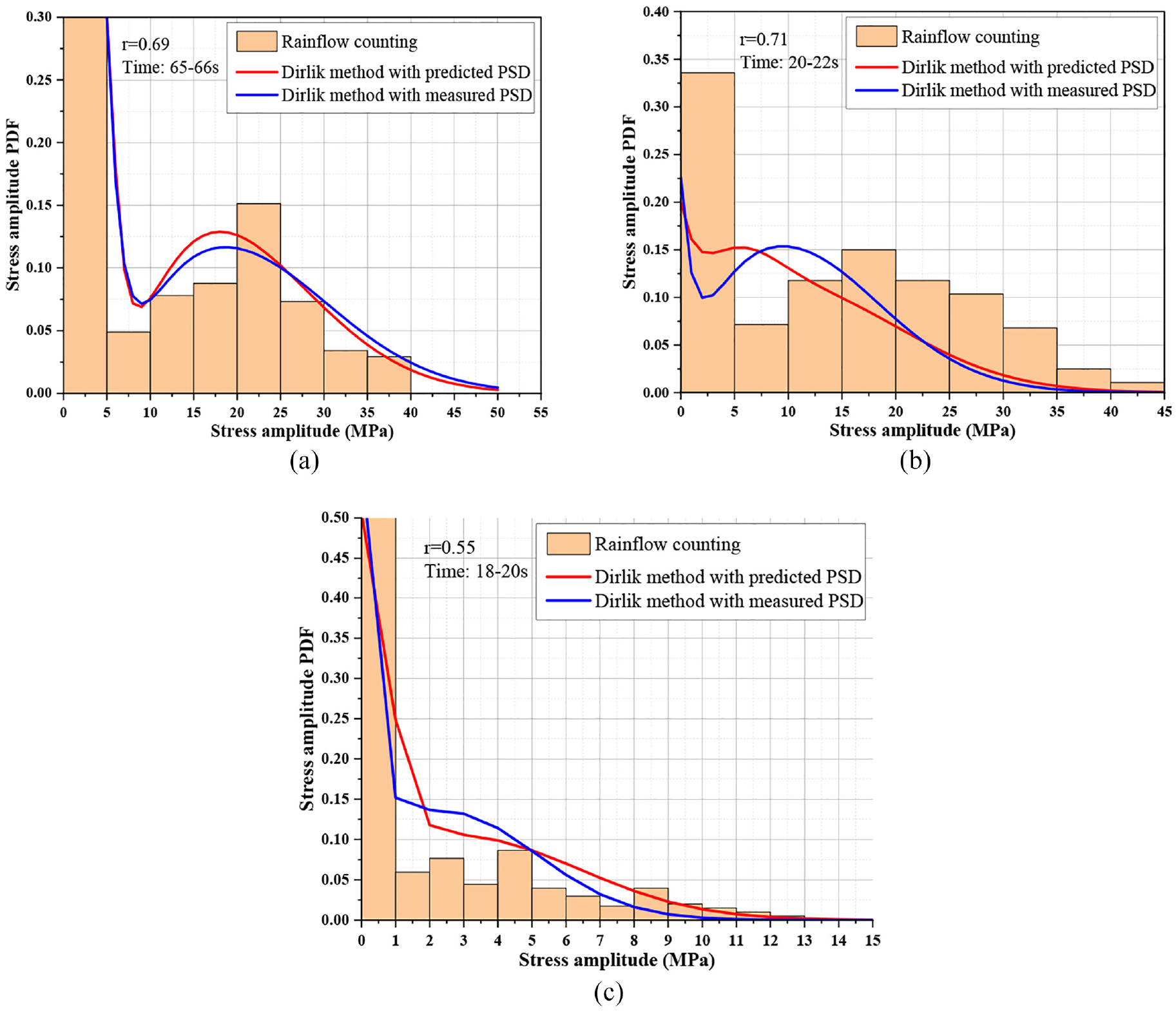
Comparisons of stress amplitude PDFs of both measured and predicted results using RFC method and Dirlik method in different sections: (a) 65~66s; (b) 20~22s and (c) 18~20s.

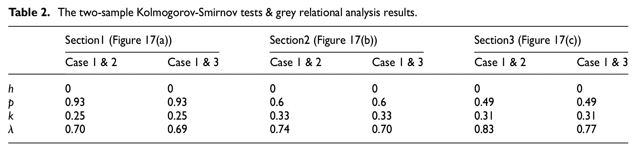
To verify the fitting effect between the predicted PDFs and the measured ones as shown in Figure 17, the two-sample Kolmogorov-Smirnov tests⁴⁷ and grey relational analysis are conducted. As shown in Table 2, case 1–3 represent the PDFs from the RFC method, and the Dirlik method using predicted PSDs and measured PSDs, respectively. The test results corresponding to the three sections shown in Figure 17(a) to (c) are illustrated, where h, p and k denote the hypothesis test result, the asymptotic p-value and the test statistic values. The null hypothesis (h = 0) has all been accepted at the significant level of 0.01 which proves that the predicted and measured PDFs are from the same distribution.

Table 2.

The two-sample Kolmogorov-Smirnov tests & grey relational analysis results.

	Section1 (Figure 17(a))		Section2 (Figure 17(b))		Section3 (Figure 17(c))
	Case 1 & 2	Case 1 & 3	Case 1 & 2	Case 1 & 3	Case 1 & 2	Case 1 & 3
h	0	0	0	0	0	0
p	0.93	0.93	0.6	0.6	0.49	0.49
k	0.25	0.25	0.33	0.33	0.31	0.31
λ	0.70	0.69	0.74	0.70	0.83	0.77

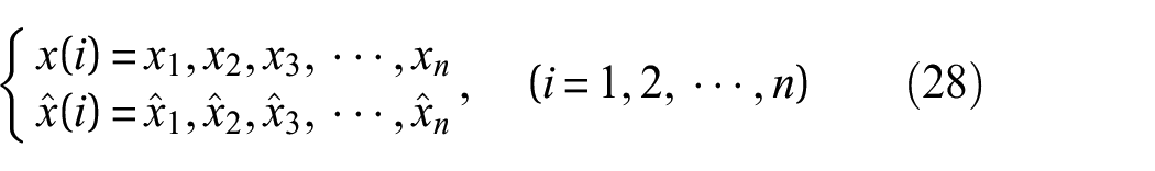
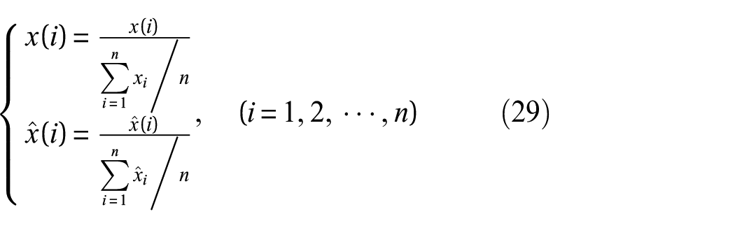
On the other hand, the grey relational analysis⁴⁸ is used to characterize the numerical proximity of two sequences. The two original sequences in Equation (28) could be normalized using the averaging method as shown in Equation (29).

{\begin{matrix} x (i) = x_{1}, x_{2}, x_{3}, \dots, x_{n} \\ \hat{x} (i) = {\hat{x}}_{1}, {\hat{x}}_{2}, {\hat{x}}_{3}, \dots, {\hat{x}}_{n} \end{matrix}, (i = 1, 2, \dots, n)

(28)

{\begin{matrix} x (i) = \frac{x (i)}{\sum_{i = 1}^{n} x_{i} / n} \\ \hat{x} (i) = \frac{\hat{x} (i)}{\sum_{i = 1}^{n} {\hat{x}}_{i} / n} \end{matrix}, (i = 1, 2, \dots, n)

(29)

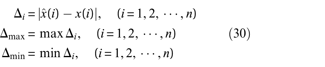
Then the deviation sequence Δ_i of the reference sequence and the comparability sequence is obtained in Equation (30). Δ_max and Δ_min are the maximum and minimum value of the Δ_i.

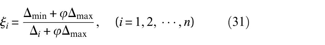
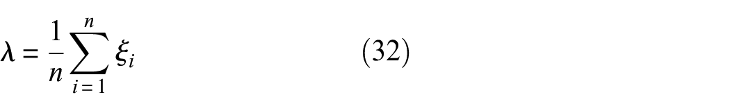
\begin{matrix} Δ_{i} = & | \hat{x} (i) - x (i) |, (i = 1, 2, \dots, n) \\ Δ_{max} = & max Δ_{i}, (i = 1, 2, \dots, n) \\ Δ_{min} = & min Δ_{i}, (i = 1, 2, \dots, n) \end{matrix}

(30)

The grey relation coefficient ξ_i can be expressed in Equation (31). ξ is the distinguishing coefficient between 0 and 1, which can be adjusted according to different actual system requirements. The smaller the value of ζ is, the distinguished ability becomes larger. ζ = 0.5 is generally used.⁴⁸ Then the average value of the grey relational coefficients is taken as the grey relational degree λ as shown in Equation (32).

ξ_{i} = \frac{Δ_{min} + φ Δ_{max}}{Δ_{i} + φ Δ_{max}}, (i = 1, 2, \dots, n)

(31)

λ = \frac{1}{n} \sum_{i = 1}^{n} ξ_{i}

(32)

The grey relational degree results are shown in Table 2. It can be seen that the results in the three sections are larger than 0.69. In general, the fitting effect between the predicted PDFs and the measured ones is good.

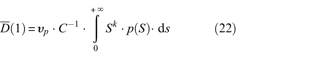
So the calculated results from predicted PSDs and measured PSDs are consistent and the errors are acceptable. The fatigue damage could then be calculated by the frequency domain method based on Equation (22). On the other hand, the real-time stress could also be obtained based on the predicted PSDs.

After obtaining the concerned stress PSD, the stress time history could then be reconstructed using the IFFT using the uniformly distributed random phases at different frequencies. As shown in Figure 18(a) and (b), the reconstructed Y-axis stress time histories at the concerned point are quite comparable to the measured results. In some time segments, the predicted results could be larger than the measured ones, which could arise from the amplitude differences at some frequencies of the PSDs.

Figure 18.

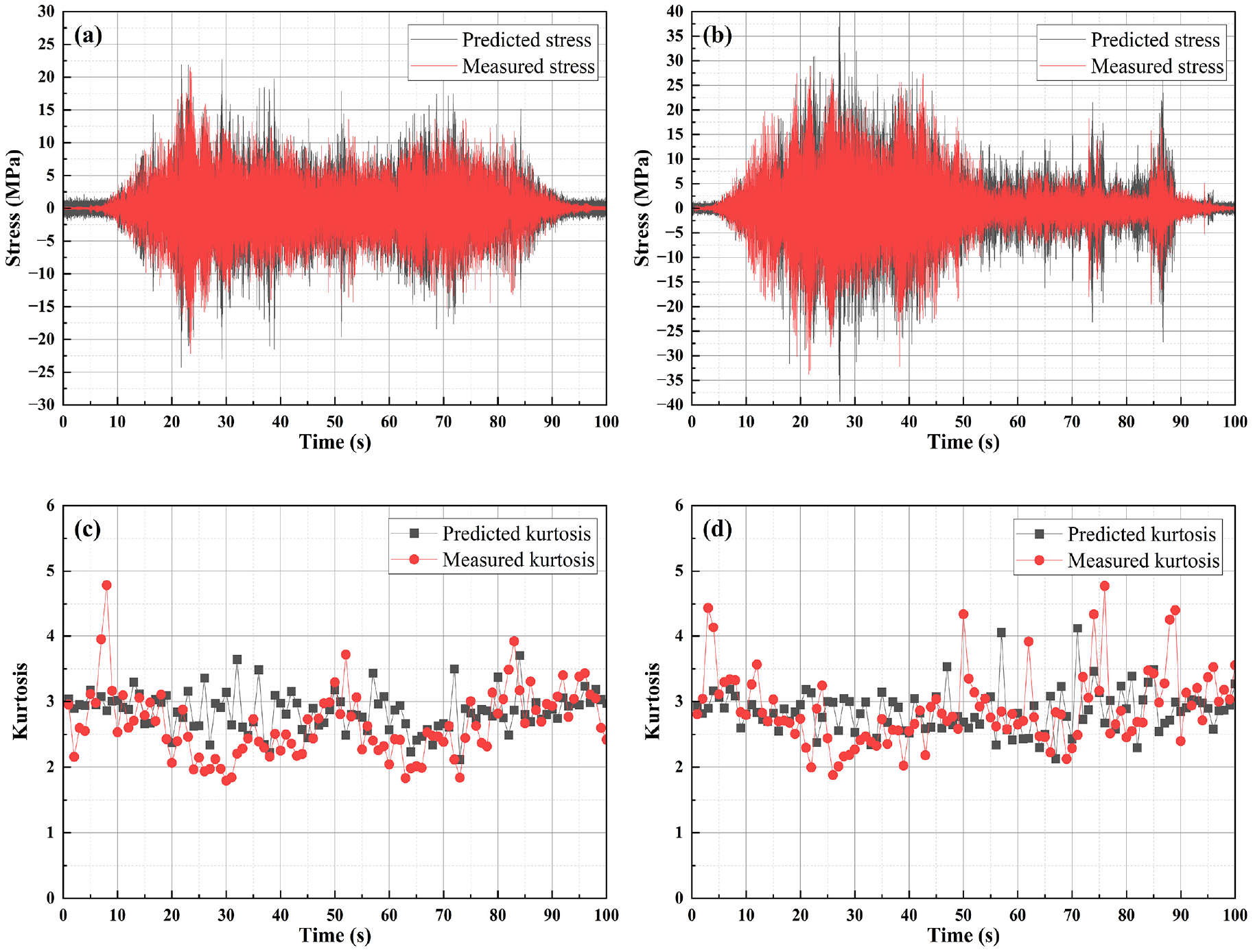
Comparisons of measured and predicted results: (a), (b) dynamic stress and (c), (d): time-varying kurtosis.

The non-normality of the dynamic stress will lead to an underestimation of the stress amplitudes in the process of stress reconstruction. In light of the central limit theorem, the reconstructed signal tends to be a normal distribution due to the employment of uniformly distributed random phases at different frequencies. The previous studies pointed out that changing the randomness of the uniformly distributed random phases at different frequencies will strengthen the fluctuating features such as the sharp spike events of the signal and further increase the kurtosis value of the signal.⁴⁹ But as shown in Figure 18(c) and (d), the time-varying kurtosis in each time segment of 1 s presents less obvious non-normal characteristics. That means the influence of the signal’s non-normality on stress reconstruction is not obvious in this study.

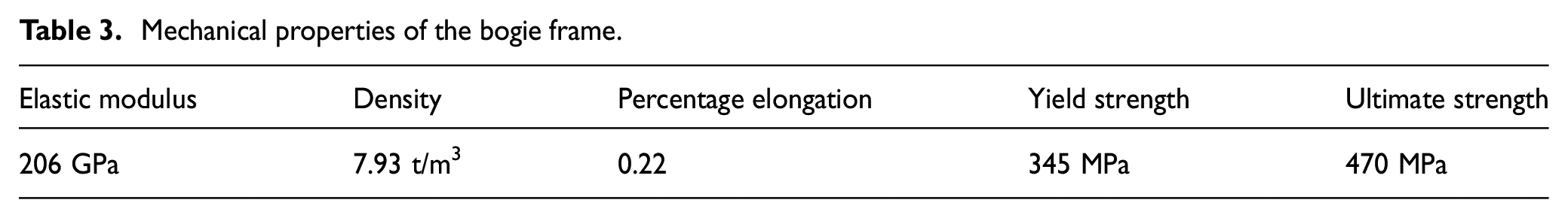
Based on the estimated stress PSDs, the PDFs of the stress range could be obtained in each segment. The whole fatigue damage could be calculated using the S–N curve in power exponent form with a reliability of 99%. The material property of the bogie frame is illustrated in Table 3. The RFC method using the linear Miner’s rule as well as the Dirlik method are employed to conduct the validation. The value of m in the S–N curve is 3.5 and a fatigue limit of 70 MPa with the corresponding number of cycles N = 2 × 10⁶ cycles is suggested which is widely used for bogie frame in this paper.⁵⁰ As shown in Table 4, the damage calculated from the RFC method in different sections which are corresponding to Figure 18(a) and (b) is lower than that from the Dirlik method and the deviations are within 22%.

Table 3.

Mechanical properties of the bogie frame.

Elastic modulus	Density	Percentage elongation	Yield strength	Ultimate strength
206 GPa	7.93 t/m³	0.22	345 MPa	470 MPa

Table 4.

The fatigue damage of the bogie frame.

Damage	RFC method	Dirlik method
Section1 (Figure 17(a))	2.36e-5	2.86e-5
Section2 (Figure 17(b))	8.53e-5	1.08e-4

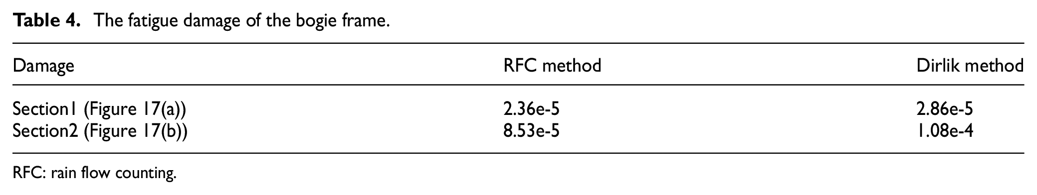
RFC: rain flow counting.

In previous research, the application of the measured dynamic stress spectra is limited to the classical damage accumulation design. However, some researchers^51,52 have proposed the advanced damage tolerance philosophy for railway bogies which are mainly based on standard prescribed loads or measured loads. The damage results considering the crack propagation will be more accurate and more conservative compared with the conventional safety life design. So the fatigue crack propagation under the estimated stress time histories and the measured ones are compared for validations of the proposed methodology. In general, the rate of the fatigue crack propagation during the stable propagation period (in Paris regime) can be described by the Paris equation.⁵³ The relationship between the fatigue crack growth rate (da/dN) and the stress intensity factor (SIF) range (ΔK) can be described as follows:

d a / d N = C \cdot (Δ K)^{m}

(33)

Δ K = f \cdot Δ σ \cdot \sqrt{π a}

(34)

where C and m are constants which are related to the material property; f denotes the shape coefficient of SIF and Δσ represents the stress range of each level; a is the length of the fatigue crack.

After integrating the Equation (33), it can be obtained:

N = \int_{a_{0}}^{a_{c}} \frac{d a}{C {(Δ K)}^{m}}

(35)

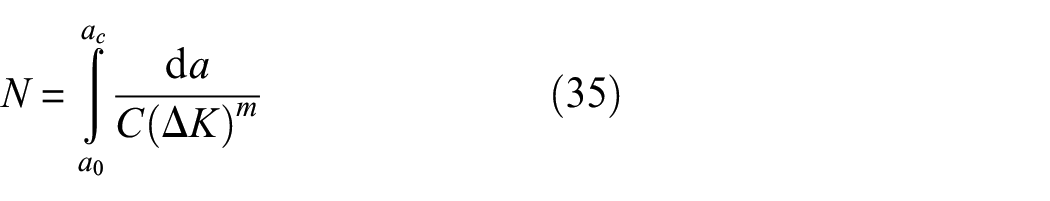
where a₀ is the initial crack size and a_c is the critical crack length.

When substituting Equation (34) into Equation (35), the critical crack length could be calculated as:

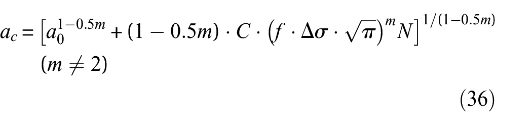
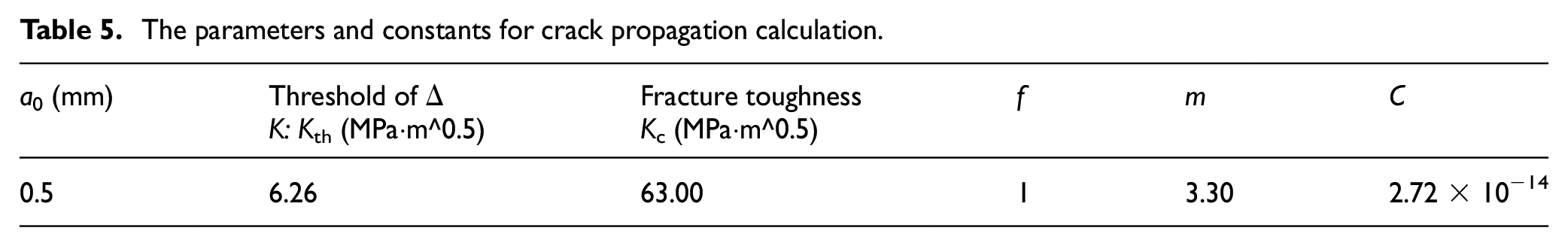
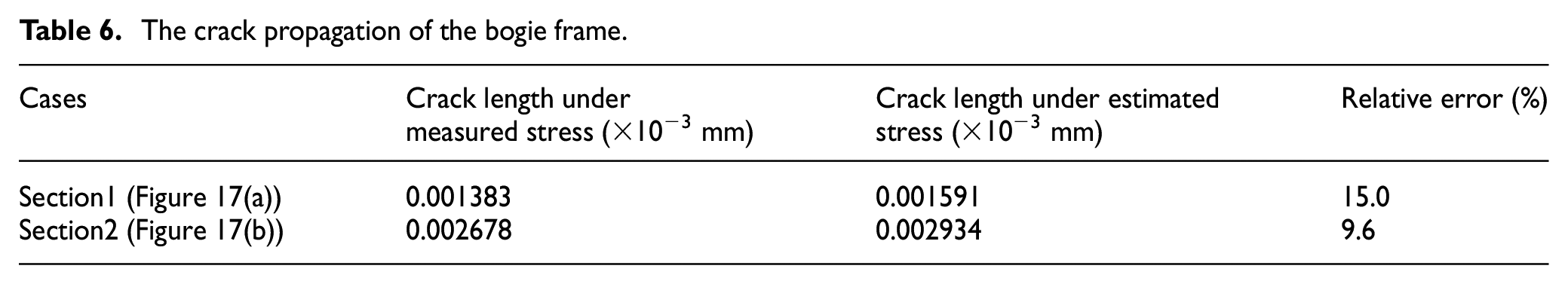
\begin{matrix} a_{c} = {[a_{0}^{1 - 0.5 m} + (1 - 0.5 m) \cdot C \cdot {(f \cdot Δ σ \cdot \sqrt{π})}^{m} N]}^{1 / (1 - 0.5 m)} \\ (m \neq 2) \end{matrix}

(36)

The parameters mentioned above are listed in Table 5. The initial crack length a₀ is assumed to be 0.5 mm, which is the minimum detectable crack size by the magnetic particle testing. The stress time series in Figure 18(a) and (b) are transformed into different stress range levels Δσ_i by RFC method. The crack growth quantity a_i under Δσ_i with the cycles N_i could be calculated by Equation (36). And a₀ is replaced by a_i when calculating a_i_+ 1 under the stress range Δσ_i_+ 1 with the cycles N_i_+ 1. The crack propagation lengths under the measured and estimated stress in Figure 18(a) and (b) are listed in Table 6. It can be seen that the relative errors with respect to the measured results are 15% and 9.6% respectively.

Table 5.

The parameters and constants for crack propagation calculation.

a ₀ (mm)	Threshold of ΔK: K_th (MPa·m^0.5)	Fracture toughnessK_c (MPa·m^0.5)	f	m	C
0.5	6.26	63.00	1	3.30	2.72 × 10⁻¹⁴

Table 6.

The crack propagation of the bogie frame.

Cases	Crack length under measured stress (×10⁻³ mm)	Crack length under estimatedstress (×10⁻³ mm)	Relative error (%)
Section1 (Figure 17(a))	0.001383	0.001591	15.0
Section2 (Figure 17(b))	0.002678	0.002934	9.6

Conclusion

In this study, the scheme of the fatigue stress estimation of the metro bogie frame is presented for monitoring certain types of modal vibration. The proposed algorithm depends on frequency domain methods with a preceding procedure of transfer path analysis, which consists of analysis in the time domain and coherence analysis in the frequency domain. Some conclusions can be drawn as follows:

As one of the most common modal vibrations of metro bogie frame, the transom bending deformation is easily excited due to P2 resonance arising from wheel/rail interactions. The coherence analysis reveals that the vertical axle box acceleration is the main contributor to the fatigue damage of the transom. The analysis also found that an erroneous high coherence may exist due to the high coherence between the inputs. The influence of the secondary suspension loads from the car body has been analyzed using both MSC and PDC analysis. And the results reveal that only the MSC analysis cannot reflect the true relationships between the secondary suspension loads and the stress of the bogie frame. With the aid of PDC analysis and other methods, a comprehensive analysis is helpful to remove irrelevant excitations for computational convenience.

The four axle box vertical accelerations are obtained through the onboard device and its PSDs are calculated in real time within each time interval. The transfer function of the Y-axis stress to axle box accelerations could be calculated in advance. Then the estimated dynamic stress PSDs are obtained and the results show a good agreement with the measured results. Both the stress amplitude distributions calculated from measured and predicted stress PSDs using the Dirlik method are identical to the RFC results. Both the classical damage accumulation design and the advanced damage tolerance philosophy are used for railway bogies. And the fatigue damage errors between the estimated results and the measured results are within 20%.

Compared with the vertical axle box accelerations which possess the irregularity index lower than 0.5, the Y-axis dynamic stress tends to be the narrow-band process. The stress range below 5 MPa is always dominant. With the increase of the irregularity index, the proportion of stress ranges from 10 to 40 MPa obviously increases, which contributes most to the fatigue failure of the bogie frame. The stress reconstruction results based on IFFT show good consistency with the measured results. The non-normal characteristics of the whole process are not considered in this study. During the short time interval, the non-normal characteristics of the dynamic stress are not obvious and the deviation with real damage needs further study. In general, the stability and computing efficiency are ensured for the proposed methodology.

Footnotes

Declaration of conflicting interests

The author(s) declared no potential conflicts of interest with respect to the research, authorship, and/or publication of this article.

Funding

The author(s) disclosed receipt of the following financial support for the research, authorship, and/or publication of this article: This project is partially supported by the National Natural Science Foundation of China (Grant No. 52002344; 51975485; 61960206010) and the Independent Project of State Key Laboratory of Traction Power (Grant No. 2022TPL-T09).

ORCID iDs

Yi Sun

Lai Wei

References

Cole

Spiryagin

. Track maintenance reactions for combined track defects. ICRT 2021. Reston, VA: American Society of Civil Engineers, 2022, pp. 9–15.

Zhai

Jin

Wen

, et al. Wear problems of high-speed wheel/rail systems: observations, causes, and countermeasures in China. Appl Mech Rev 2020; 72(6): 060801.

Zeng

, et al. Vibration fatigue dynamic stress simulation under multi-load input condition: application to metro lifeguard. Eng Fail Anal 2019; 99: 141–152.

Xie

Liu

, et al. Study on high frequency vibration-induced fatigue failure of antenna beam in a metro bogie. Eng Fail Anal 2022; 133: 105976.

Wang

Yang

, et al. An experimental investigation of the mechanism and mitigation measures for the coil spring fracture of a locomotive. Eng Fail Anal 2022; 135: 106157.

Zhou

Chi

Wen

, et al. An investigation of abnormal vibration–induced coil spring failure in metro vehicles. Eng Fail Anal 2020; 108: 104238.

Wang

Dong

. Analysis on the fatigue cracks in the bogie frame. Eng Fail Anal 2015; 58: 307–319.

Sun

Wei

Liu

, et al. Dynamic stress analysis of a metro bogie due to wheel out-of-roundness based on multibody dynamics algorithm. Eng Fail Anal 2022; 134: 106051.

, et al. Fatigue analysis of the gearbox housing in high-speed trains under wheel polygonization using a multibody dynamics algorithm. Eng Fail Anal 2019; 100: 351–364.

10.

Zhi

Wang

Tian

, et al. Fracture mechanism analysis and design optimization of a wheelset lifting mechanism based on experiments and simulations. Machines 2022; 10(5): 397.

11.

Guo

, et al. Current signal characteristics analysis of transmission system in high-speed train under abnormal vibration conditions. Veh Syst Dyn 2022; 61(4): 1151–1167.

12.

Peng

Zeng

Wang

, et al. Wayside wheel-rail vertical contact force continuous detecting method and its application. Measurement 2022; 193: 110975.

13.

Milković

Simić

Jakovljević

, et al. Wayside system for wheel–rail contact forces measurements. Measurement 2013; 46(9): 3308–3318.

14.

Bosso

Gugliotta

Zampieri

. Wheel flat detection algorithm for onboard diagnostic. Measurement 2018; 123: 193–202.

15.

Wei

Liu

Jia

. Urban rail track condition monitoring based on in-service vehicle acceleration measurements. Measurement 2016; 80: 217–228.

16.

De Oliveira

Loprencipe

Almeida

Filho

FGV

, et al. Experimental investigation on the use of multiple very low- cost inertial-based devices for comfort assessment and rail track monitoring. Measurement 2022; 199: 111549.

17.

Hong

Wang

, et al. In situ health monitoring for bogie systems of CRH380 train on Beijing–Shanghai high-speed railway. Mech Syst Signal Process 2014; 45(2): 378–395.

18.

Gao

Wen

, et al. Online estimation of fatigue damage of railway bogie frame based on axle box accelerations. Veh Syst Dyn 2023; 61: 286–308.

19.

Ugras

Alkan

Orhan

, et al. Real time high cycle fatigue estimation algorithm and load history monitoring for vehicles by the use of frequency domain methods. Mech Syst Signal Process 2019; 118: 290–304.

20.

Cai

Zhang

Liang

, et al. Localization and image of metro vehicle bogie frame using guided waves. Wireless Netw 2022; 28: 2323–2335.

21.

Xiu

Spiryagin

, et al. Fatigue life assessment methods for railway vehicle bogie frames. Eng Fail Anal 2020; 116: 104725.

22.

Liu

Song

, et al. Development method and experimental verification of fatigue load spectrum of anti-yaw damper for rail vehicles. Eng Fail Anal 2022; 138: 106298.

23.

Liu

, et al. An investigation into vibration-induced fatigue failure of metro vehicle cowcatcher and its structural improvement design. Eng Fail Anal 2023; 145: 107038.

24.

Wei

Sun

Zeng

, et al. Experimental and numerical investigation of fatigue failure for metro bogie cowcatchers due to modal vibration and stress induced by rail corrugation. Eng Fail Anal 2022; 142: 106810.

25.

Mei

Luo

Qiao

, et al. Study of load spectrum compilation method for the pantograph upper frame based on multi-body dynamics. Eng Fail Anal 2022; 135: 106099.

26.

You

Zhou

Gong

, et al. Synthesis of random vibration environment spectra for the fatigue analysis and optimization of railway vehicles. Int J Fatigue 2022; 159: 106752.

27.

Dirlik

Benasciutti

. Dirlik and tovo-benasciutti spectral methods in vibration fatigue: a review with a historical perspective. Metals 2021; 11(9): 1333.

28.

Wolfsteiner

Breuer

. Fatigue assessment of vibrating rail vehicle bogie components under non-Gaussian random excitations using power spectral densities. J Sound Vib 2013; 332(22): 5867–5882.

29.

Dou

Liu

Mao

. Synthesis approach of multiaxial vibration test profile for non-Gaussian excitation. J Mech Sci Technol 2021; 35(12): 5309–5321.

30.

British Standards Institution. Railway applications–rolling stock equipment-shock and vibration test. BS EN 61373:2010. London, England: BSI, 2010.

31.

Xiang

Dong

, et al. Analysis of the effects of vibration modes on fatigue damage in high-speed train bogie frames. Eng Fail Anal 2018; 89: 222–241.

32.

Guo

, et al. Influence of DC-link voltage pulsation of transmission systems on mechanical structure vibration and fatigue in high-speed trains. Eng Fail Anal 2021; 130: 105772.

33.

Baccalá

Sameshima

. Partial directed coherence: a new concept in neural structure determination. Biol Cybern 2001; 84(6): 463–474.

34.

Baccalá

Sameshima

. Frequency domain repercussions of instantaneous Granger causality. Entropy 2021; 23(8): 1037.

35.

Wang

Tang

. Exact confidence interval for magnitude-squared coherence estimates. IEEE Signal Process Lett 2004; 11(3): 326–329.

36.

Welch

. The use of fast Fourier transform for the estimation of power spectra: a method based on time averaging over short, modified periodograms. IEEE Trans Audio Electroacoust 1967; 15(2): 70–73.

37.

Bendat

Piersol

. Random data: analysis and measurement procedures. Hoboken, NJ: John Wiley & Sons, 2011.

38.

Ter Wal

Cardellicchio

LoRusso

, et al. Characterization of network structure in stereoEEG data using consensus-based partial coherence. Neuroimage 2018; 179: 385–402.

39.

Sameshima

Baccalá

. Methods in brain connectivity inference through multivariate time series analysis. Boca Raton, FL: CRC Press, 2014.

40.

Baccalá

Sameshima

. Partial directed coherence: twenty years on some history and an appraisal. Biological Cybernetics 2021; 115(3): 195–204.

41.

Lalanne

. Mechanical vibration and shock analysis, fatigue damage. Hoboken, NJ: John Wiley & Sons, 2014.

42.

Newland

. An introduction to random vibrations, spectral & wavelet analysis. New York: Dover Publications, 2012.

43.

Ibrahim

. Parametric random vibration. New York: Dover Publications, 2008.

44.

Zalaznik

Nagode

. Frequency based fatigue analysis and temperature effect. Mater Des 2011; 32(10): 4794–4802.

45.

Capponi

Česnik

Slavič

, et al. Non-stationarity index in vibration fatigue: theoretical and experimental research. Int J Fatigue 2017; 104: 221–230.

46.

. Vibration fatigue dynamic stress simulation under non-stationary state. Mech Syst Signal Process 2021; 146: 107006.

47.

Massey

. The Kolmogorov-Smirnov test for goodness of fit. J Am Stat Assoc 1951; 46(253): 68–78.

48.

Tosun

. Determination of optimum parameters for multi-performance characteristics in drilling by using grey relational analysis. Int J Adv Manuf Technol 2006; 28(5): 450–455.

49.

Jiang

Tao

Chen

, et al. Non-Gaussian random vibration fatigue analysis and accelerated test. Singapore: Springer Singapore Pte. Limited, 2021.

50.

Wang

Sun

, et al. Fatigue damage and reliability assessment of subway train bogie frames under operating conditions. Adv Mech Eng. Epub ahead of print 1 January 2014. DOI: 10.1177/1687814020903590.

51.

Guo

Liu

, et al. An innovative stepwise time-domain fatigue methodology to integrate damage tolerance into system dynamics. Veh Syst Dyn 2023; 61(2): 550–572.

52.

Yang

Duan

, et al. Damage tolerance assessment of a brake unit bracket for high-speed railway welded bogie frames. Chin J Mech Eng 2019; 32: 1–11.

53.

Yang

Sun

Zheng

, et al. Revealing the correlation between microstructure and fatigue crack growth behaviors in Ti–6Al–3Nb–2Zr–1Mo alloy. Mater Sci Eng: A 2022; 848: 143406.

Fatigue stress estimation of metro bogie frame through frequency response functions by using limited sensors

Abstract

Keywords

Introduction

In situ investigation of the bogie frame fracture

Background

Motivation

Analysis of different loads’ influences on the stress state of the bogie frame

Methodologies

Acquisition of transfer functions and estimation of the dynamic stress spectrum

The fatigue stress estimation using the frequency domain method

A case study of the metro bogie frame

Transfer property analysis of the bogie system

Fatigue stress estimation and damage evaluation

Conclusion

Footnotes

Declaration of conflicting interests

Funding

ORCID iDs

References